| Issue |
A&A
Volume 522, November 2010
|
|
|---|---|---|
| Article Number | A31 | |
| Number of page(s) | 8 | |
| Section | The Sun | |
| DOI | https://doi.org/10.1051/0004-6361/201014052 | |
| Published online | 28 October 2010 | |
Acoustic waves in the solar atmosphere at high spatial resolution
II. Measurement in the Fe i 5434 Å line
1
Kiepenheuer-Institut für Sonnenphysik,
Schöneckstr. 6,
79104
Freiburg,
Germany
e-mail: This email address is being protected from spambots. You need JavaScript enabled to view it.
2
Institut für Astrophysik, Friedrich-Hund-Platz 1, 37077
Gottingen,
Germany
e-mail: This email address is being protected from spambots. You need JavaScript enabled to view it.
; This email address is being protected from spambots. You need JavaScript enabled to view it.
3
Central Astronomical Observatory, Russian Academy of Sciences,
Pulkovskoye chaussee 65/1,
196140
St. Petersburg,
Russia
4
Main Astronomical Observatory, National Academy of Sciences,
Golosiiv, 03680,
Kyiv -
127,
Ukraine
e-mail: This email address is being protected from spambots. You need JavaScript enabled to view it.
Received:
12
January
2010
Accepted:
27
May
2010
Abstract
Aims. We investigate the energy supply of the solar chromosphere by acoustic waves.
Methods. A time sequence with high spatial and temporal resolution from the quiet Sun disc centre in Fe i 5434 Å (Landé factor g = 0) is analysed. We used models from a numerical simulation of granular convection and apply NLTE spectral line transfer to determine the height of formation. For estimates of acoustic energy flux, we adopted wave propagation with inclinations of the wave vector with respect to the vertical of 0°, 30°, and 45°. For a granular and an intergranular model, the transmissions of the atmosphere to high-frequency waves were determined for the three inclination angles. Wavelet and Fourier analyses were performed and the resulting power spectra were corrected for atmospheric transmission.
Results. We find waves with periods down to ~40 s. They occur intermittently in space and time. The velocity signal is formed at a height of 500 km in the granular model and at 620 km in the intergranule. At periods shorter than the acoustic cutoff (~190 s), ~40% of the waves occur above granules and ~60% above intergranules. By adopting vertical propagation, we estimate total fluxes above granules of 2750–3360 W m-2, and of 910–1 000 W m-2 above intergranules. The weighted average is 1730–2 060 W m-2. The estimates of the total fluxes increase by 15% when inclined wave propagation of 45° is assumed.
Key words: Sun: chromosphere / Sun: oscillations / techniques: spectroscopic / Sun: photosphere
© ESO, 2010
1. Introduction
This contribution deals with the problem of the energy supply of the solar chromosphere. In our recent work, Bello González et al. (2009b, henceforth Paper I), we studied the acoustic flux in short-period waves by means of observations in the Fe i 5576 Å line. The formation height of the velocity signal in this line was determined to 250 km in the VAL C model of Vernazza et al. (1981). We found an acoustic energy flux of ~3000 W m-2, a factor of 4–6 larger than given by Fossum & Carlsson (2006) and Carlsson et al. (2007) from intensity fluctuations in continuum bands at 1600 Å and in Ca ii H formed at heights of 430 km and 200 km, respectively. We refer the reader to Paper I for a discussion of the arguments for and against acoustic wave heating.
Here we present results from wave observations in Fe i 5434 Å. This line, with Landé factor gL = 0, is commonly assumed to be formed around the temperature minimum region of standard models. As we show below, the velocity signal at line minimum of Fe i 5434 Å is formed at atmospheric heights of 400–650 km, i.e. much higher than the velocity signals of Fe i 5576 Å analysed in Paper I. It is thus interesting to use the same method as in Paper I to estimate, from two-dimensional spectroscopy and with speckle reconstruction, the energy flux carried by short-period waves at high photospheric layers. One may then see how much flux survives the radiative dissipation in the photosphere and is available as an energy supply from acoustic waves for chromospheric radiation.
Apart from the important issue of chromospheric heating, we extend the present study beyond the analyses in Paper I: 1) For the estimates of acoustic energy fluxes, we assume not only vertically propagating waves but also allow oblique propagation. 2) The estimates were performed for both granular and intergranular atmospheric models from numerical simulations by Asplund et al. (2000). 3) NLTE calculations of Fe ionisation and of the Fe i 5576 Å line formation as in Shchukina & Trujillo Bueno (2001) were applied to determine the heights of formation of this line in granules and intergranules.
After the description of the observations and the data analysis in Sect. 2, we give in Sect. 3.1 the equations for propagation of linear adiabatic waves that travel obliquely in an isothermal atmosphere. Then we use convection models from numerical simulations to determine the height of formation of the velocity signal and the transmissions with NLTE radiative transfer in an intergranular and granular model (Sects. 3.2 and 3.3, respectively). The results are discussed in Sect. 4 for wavelet and Fourier analyses. Section 5 concludes the paper.
2. Observations and data analysis
The observations were taken on May 12, 2009, from the quiet disc centre of the Sun. We used the Göttingen Fabry-Perot spectrometer (FPI) with its upgrades (Puschmann et al. 2006; Bello González & Kneer 2008) at the Vacuum Tower Telescope/Observatorio del Teide/Tenerife. The observations were supported by the Kiepenheuer Adaptive Optics System (KAOS, von der Lühe et al. 2003). We use here a time sequence of 24 min duration of scanning through Fe i 5434 with a cadence of 15.5 s. The Fried parameter r0 was 8–18 cm. The pre-filter for the FPI, with central transmission of 0.7, had an FWHM of 6 Å. Eight frames, with pixel size corresponding to 0″̣109 × 0″̣109, were recorded at each of 36 wavelength positions with a separation of 15.63 mÅ and exposure times of 7 ms. Broadband frames at 5434 Å (through a filter with FWHM ~50 Å) were recorded simultaneously with the narrow-band images.
The images were reconstructed with our speckle code (de Boer 1996; Bello González et al. 2005) and subjected to the same processing as in Paper I with a few modifications.
-
1.
The reconstructed images of the broadband time sequencewere aligned and destretched before they were used for thereconstruction of the narrow-band images. At an early stage of theanalysis, this yields a smooth sequence of the broadband images,or a movie. Consequently, the movies from the narrow-band data,e.g. velocities, line minimum, and continuum intensities, etc,also appear smooth and need only a little destretching, if any.
-
2.
We improved substantially the effect of the intensity fluctuations along the wavelength caused by the FPI spectrometer, mentioned by, e.g. Bello González & Kneer (2008,see their Fig. 1 and the discussion to it). In Paper I we had to apply a broad wavelength filter during the analysis (see Fig. 2 in the Appendix there). This moved the formation height of the velocity signal down in the atmosphere and broadened the velocity response function. In the present study, for smoothing in wavelength, it was sufficient to convolve the line profiles with the Hamming function SH = [0.26, 0.48, 0.26].
-
3.
The reconstructed and destretched narrow-band sequences from each wavelength position were shifted to the identical starting time of each scan. From tests we have seen that this has no effect on the present study where we measure velocities from line minimum shifts. But it should become standard and will be important if one deals with measurements involving distant parts in a line profile, such as continuum intensities, line shifts from bisectors, or velocities from different spectral lines scanned sequentially.
-
4.
We determined the line minimum intensities and positions, for measuring the Doppler shifts or line-of-sight (LOS) velocities, in the following way. The Fourier transforms of the profiles were padded with zeros to 100 times more points beyond the Nyquist frequency. Then we transformed back and determined the minimum position and intensity from the parabola through the three intensities around minimum. This is another method of interpolation, which we find convenient and more accurate than quadratic interpolation or interpolation with splines, especially when the line profiles are very asymmetric as in some cases of our observations of this strong Fe i 5434 Å line.
The time sequences from each pixel were apodised with cosine bells over six time steps, i.e. over 93 s, at the beginning and at the end. The observed area was very quiet. The line minimum intensities did not even show any persistent brightening, that would be expected from network areas.
Figure 1 depicts Fe i 5434 Å profiles. We present profiles calculated in NLTE from atmospheres resulting from numerical simulations of granular convection by Asplund et al. (2000), one profile from a granule (in short GR), the other from an intergranular space (IGR). Also the effects of the finite resolution of the spectrograph and by the smoothing with the Hamming function are shown. Near continuum wavelength, the profiles differ by 37% relative to their average. Around line minimum, the GR profile is more affected by the measuring process than the IGR profile. The GR model gives a lower source function at the formation height of line minimum than the IGR model. There the GR source function is almost constant, it shows even a small increase with height. This results in a redshifted line minimum for a perturbation with upward velocity. Figure 1 also shows the average observed profile. The model of granular convection does not contain waves, and the observed profile is contaminated by false light from the side lobes of the FPI. The false light here is not as intense as in our earlier observations of the Fe i 5576 Å line (see the Appendix of Paper I), and it has a negligible influence on the velocity measurements.
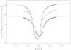 |
Fig. 1 Fe i 5434 Å profiles for the atmospheres from numerical simulations by Asplund et al. (2000). The solid line and rhombs: from granule (GR) with infinite spectral resolution and after convolving with FPI spectrometer curve and Hamming smoothing, respectively; dashed and asterisks: the same for intergranular (IGR) area; crosses: average observed profile scaled to the average of the calculated intensities in the wings. |
We restricted the study to a field of view (FOV) of 35″ × 23″ around the AO lockpoint. The time sequence of velocities in this FOV was subjected to a high-pass filter, which transmits only waves in the acoustic domain and with horizontal wavelength ≤ 10″ (cf. Paper I and Straus et al. 2008).
On the one hand, the high-pass filtering in wavelength removes noise on and near the frequency axis. As we have seen during the data analysis, this “noise” arises from temporal fluctuations of the line minimum position averaged over the rather small FOV. They occur because velocities with large amplitudes at high atmospheric layers produce line profiles with large asymmetries, which are barely noticed in the average profiles. As a consequence, the average line minimum position varies from one time step to the next.
On the other hand, the filtering also removes solar signal at small horizontal wavelengths. We recall that waves of small horizontal extent of a few arcsec also produce a power signal at small horizontal wavenumbers in the diagnostic diagram, i.e. in the kx − ν plane. Vice versa, vertically propagating waves with small horizontal extent produce signal also at large horizontal wavenumbers, which thus does not necessarily indicate oblique propagation. We estimate the loss of power by the filtering from the solar signal to 10–20%, since most of the observed signals possess a horizontal extent of typically 1″. We show below a flux spectrum in which we have retained the large scales.
3. Wave propagation, response functions, and atmospheric transmission
3.1. Equations of wave propagation
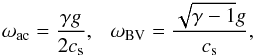
We treat adiabatic propagation of plane waves in the stratified, solar atmosphere, which we assume isothermal. Let be ω = 2πν the angular frequency, kx and kz are the horizontal and vertical components of the wave vector, respectively, with real (ω,kx,kz). The acoustic cutoff frequency ωac, and the Brunt-Väisälä frequency ωBV are given by
 (1)
(1)
where
γ = 5 / 3 is the ratio of specific heats,
g the surface gravity acceleration, and cs
the sound velocity for which we take 7 km s-1. With this the acoustic cutoff
frequency is ωac = 3.26 × 10⁻² s-1
(cutoff period Uac = 193 s) and the Brunt-Väisälä frequency is
ωBV = 3.19 × 10⁻² s-1. The vertical
direction is taken opposite to the vector of the surface gravity. With the above sound
speed, the scale height of the density (and pressure) stratification is
H =  = (ℛT) / (μg) = 107.5 km,
with the universal gas constant ℛ and the mean molecular weight μ also
assumed independent of height.
= (ℛT) / (μg) = 107.5 km,
with the universal gas constant ℛ and the mean molecular weight μ also
assumed independent of height.
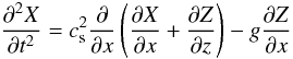
The wave equations for the particle displacements X and Z into the horizontal and vertical direction x and z, respectively, can be written as (cf. Bray & Loughhead 1974, Eq. (6.49) there)
 (2)
(2)
and
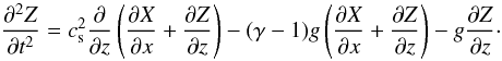 (3)
(3)
The ansatz
![Mathematical equation: \begin{equation} X = \chi\exp\left[i(\omega t-k_xx-k_zz)+ {\omega_\mathrm{ac}\over c_{\rm s}}z\right] \label{eq4} \end{equation}](/articles/aa/full_html/2010/14/aa14052-10/aa14052-10-eq35.png) (4)
(4)
and
![Mathematical equation: \begin{equation} Z = \zeta\exp\left[i(\omega t-k_xx-k_zz)+ {\omega_\mathrm{ac}\over c_{\rm s}}z\right] \label{eq5}\,, \end{equation}](/articles/aa/full_html/2010/14/aa14052-10/aa14052-10-eq36.png) (5)
(5)
with (complex) amplitudes χ and ζ, leads to the dispersion relation
 (6)
(6)
Below we assume for all frequencies (in the acoustic domain) an inclination θ of the wave vector with respect to the vertical, i.e.,
 (7)
(7)
With this, the vertical component of the phase velocity becomes
![Mathematical equation: \begin{equation} \upsilon_{{\rm ph},z} = {\omega\over k_z} = c_{\rm s}\times\left[{1+\left(1-{\omega_\mathrm{BV}^2/\omega^2}\right)\,\alpha^2 \over 1 -{\omega_\mathrm{ac}^2/\omega^2}}\right]^{1/2} , \label{eq8} \end{equation}](/articles/aa/full_html/2010/14/aa14052-10/aa14052-10-eq42.png) (8)
(8)
where we have used
the dispersion relation, Eq. (6). For high
frequencies, ω ≫ ωBV, one arrives at
υph,z(θ) = υph,z(θ = 0°)/cosθ
(see Eq. (6) of Paper I). For frequencies near the acoustic cutoff,
ω ≈ ωac, and where
ω ≈ ωBV, one gets
υph,z(θ) ≈ υph,z(θ = 0°) = ![Mathematical equation: $c_{\rm s}/[1-\omega_\mathrm{ac}^2/\omega^2]^{1/2}$](/articles/aa/full_html/2010/14/aa14052-10/aa14052-10-eq50.png) .
.
Similarly, one obtains for the vertical component of the group velocity
![Mathematical equation: \begin{equation} \upsilon_{{\rm gr},z} = {\partial\omega\over\partial k_z} = \frac{c_{\rm s}^2 / \upsilon_{{\rm ph},z}} { \left[1 - \left(\omega_\mathrm{BV}^2 / \omega^2\right) \left(c_{\rm s}^2 / \upsilon_{{\rm ph},z}^2\right) \alpha^2\right]}\cdot \label{eq9} \end{equation}](/articles/aa/full_html/2010/14/aa14052-10/aa14052-10-eq51.png) (9)
(9)
For ω ≫ ωBV one has υgr,z(θ) = υgr,z(θ = 0°)·cosθ (Eq. (7) of Paper I), while near the cutoff frequency (υph,z ≫ cs) one gets υgr,z(θ) ≈ υgr,z(θ =0°).
Finally, when we insert Eqs. (4) and (5) into the wave equations for the horizontal displacements, Eq. (2), we obtain the ratio of the moduli of the amplitudes
![Mathematical equation: \begin{equation} {\vert\chi\vert^2\over\vert\zeta\vert^2} = \tan^2\psi = {\left[k_z^2+\left({\omega_\mathrm{ac}/ c_{\rm s}}-{g/ c_{\rm s}^2}\right)^2\right]\cdot k_x^2 \over \left({\omega^2/ c_{\rm s}^2}-k_x^2\right)^2}\cdot \label{eq10} \end{equation}](/articles/aa/full_html/2010/14/aa14052-10/aa14052-10-eq57.png) (10)
(10)
We have denoted
the angle between the particle displacement and the vertical direction
with ψ. One can calculate
kx = αkz
and kz as functions of ω
from the dispersion relation. At high frequencies, where  =
=  and
where
and
where  ≫ (ωac / cs − g / cs2)2,
the amplitude ratio becomes
≫ (ωac / cs − g / cs2)2,
the amplitude ratio becomes  , or
ψ = θ.
, or
ψ = θ.
The direction of the wave vector does not enter the calculation of the response functions, but it enters the transmission in the vertical phase velocity through the angular dependence, Eq. (8), the group velocity, Eq. (9), and the rms velocity for the power spectra via the ratio of the moduli of the particle displacements | χ | 2 / | ζ | 2, Eq. (10).
In the estimates of acoustic wave flux below (Sect. 4), we use temporal power spectra, averaged over the FOV, of the observed LOS
velocities. We thus assume that we observe at each point of the FOV plane waves, possibly
of limited extent and with oblique propagation. The measured spectral power density is
 , where
Vz(ω) is the Fourier
transform of the measured velocity
υz(t) and “∗”
denotes the conjugate complex. The acoustic energy density per angular frequency interval
is
ρ | V(ω) | 2 = ρ [ | Vx(ω) | 2 + | Vz(ω) | 2 ] ,
where ρ is the mass density. With the assumption of plane waves the power
density for the vertical velocity is
| Vz(ω) | 2 ∝ | ζ | 2
and similarly for the horizontal velocity. The correction to obtain the total energy thus
follows as
| V(ω) | 2 = | Vz(ω) | 2 / cos2ψ.
, where
Vz(ω) is the Fourier
transform of the measured velocity
υz(t) and “∗”
denotes the conjugate complex. The acoustic energy density per angular frequency interval
is
ρ | V(ω) | 2 = ρ [ | Vx(ω) | 2 + | Vz(ω) | 2 ] ,
where ρ is the mass density. With the assumption of plane waves the power
density for the vertical velocity is
| Vz(ω) | 2 ∝ | ζ | 2
and similarly for the horizontal velocity. The correction to obtain the total energy thus
follows as
| V(ω) | 2 = | Vz(ω) | 2 / cos2ψ.
In estimates of acoustic flux from solar-disc centre observations, vertical wave propagation is often assumed (e.g., Deubner 1976; Mein & Schmieder 1981; Deubner & Fleck 1990; Fossum & Carlsson 2006). Mihalas & Toomre (1982) state that acoustic waves have lower horizontal than vertical velocities. Fossum & Carlsson (2006) argue that acoustic waves are refracted towards the direction of decreasing sound speed, i.e. towards the vertical direction. Following this reasoning we adopt in the estimates of acoustic flux below inclinations θ of the wave vector with respect to the vertical of 0°, 30°, and 45°.
3.2. Response functions
Here and for calculating of the atmospheric transmission of waves below, we employed atmospheric models of GR and IGR from numerical simulations of granular convection by Asplund et al. (2000). The NLTE ionisation equilibrium of Fe from Shchukina & Trujillo Bueno (2001) is also used. And NLTE transfer calculations of the Fe i 5434 Å line in the GR and IGR models were performed, which give the NLTE departure coefficients of the lower and upper level of this line.
We calculated response functions for the velocity measured at the line minima, RFυ(z), with the method by Eibe et al. (2001). They were determined for both the GR and IGR models. For the evaluation of RFυ(z) and of the atmospheric transmission (see below), the macroscopic, granular velocities were included and the NLTE departure coefficients of Fe i 5434 were kept unchanged during the application of velocity perturbations.
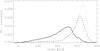 |
Fig. 2 Response functions for velocity RFυ(z) from line minimum of Fe i 5434. Dotted line: for IGR with infinite spectral resolution; solid and dashed: for GR and IGR, respectively, after convolution of line profiles with spectrometer function and Hamming function; thick solid: boxcar smoothing of thin (GR) response function over three height positions. |
Figure 2 gives the response functions for velocity in the GR and IGR models. If we assume a perfect spectrometer, the velocity response funtions RFυ(z) for the IGR peaks at a height of about 650 km. Yet applying the same spectrometric broadening and filtering in wavelength as for the observed data to the line intensities that emerge from the model atmosphere, we obtain the curves in Fig. 2 for the GR and IGR, respectively. The increase in the source function with height in the GR model impedes any calculation of the response function for infinite spectral resolution. The response functions peak at ~500 km in the GR, where the mass density in the model is ρ = 1.3 × 10⁻⁵ kg m-3, and at ~620 km in the IGR model with density ρ = 0.5 × 10⁻⁵ kg m-3.
3.3. Atmospheric transmission
As in Paper I, we calculated transmissions of velocity amplitudes, i.e. the ratio of measured to actual wave amplitude, in the GR and IGR models. We use below the square of the transmissions, the transfer functions TF, for correcting the velocity power spectra.
For calculating of the transmissions, we used the GR and IGR models and superimposed waves of small amplitude and with frequencies from 5 mHz to 34 mHz to the GR and IGR velocities. For each period/frequency we adopted the phase velocities from Eq. (8), for 25 phases between 0° and 360°. The line profiles and the velocity signals as expected from the spectrometer and the data analysis were then calculated. We determined the observable amplitudes along the 25 phases. Obviously, since the phase velocity is infinite at a frequency of 5 mHz, which is below the cutoff frequency, the transmission at this frequency is 1. For higher frequencies, the determined amplitudes were divided by the amplitude determined from the 5 mHz wave giving the transmissions at these higher frequencies.
We assumed phase velocities of vertically and obliquely propagating waves with two height
dependences of amplitude, with constant amplitude and with increasing amplitude according
to
υph(z) = υph(z = 0)·exp [ z / (2H) ] .
The latter mimics the acoustic energy flux approximately constant through the atmosphere
due to stratification. We take H = 110 km for the density scale height
(as above), which is close to
cs / (2ωac) = = 107.5 km from
Eqs. (4) and (5).
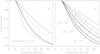 |
Fig. 3 Transmission of waves as function of wave period; a) with infinite spectral resolution for IGR (dotted) and after applying the convolution with spectrometer function and filtering; solid: for GR, dashed: for IGR; thin: for waves with amplitudes independent of height, thick: for waves with exponentially increasing amplitude; b) comparison of transmission for waves with exponentially increasing amplitude and with adopted inclination θ of 0°, 30°, and 45°; solid: GR, dashed: IGR. |
Figure 3 gives the transmissions of GR and IGR as functions of period. We adopt the period U = 190 s, which is close to the cutoff period, with transmission of 1. We first discuss Fig. 3a) with the transmissions for θ = 0°. A measurement with infinite resolution gives relatively mild corrections up to frequencies of 34 mHz. Also the transmission of the IG model is as high as ~0.25 at 34 mHz. The GR model, however, yields a very low transmission of ~0.05, hence a correction by a large factor, at high frequencies. This behaviour is reflected in the different widths of the response functions in Fig. 2. We use the transmissions calculated with an exponential height dependence of the wave amplitudes, since they yield smaller corrections than those from a constant amplitude.
Figure 3b) then shows the comparison between transmissions calculated with inclinations of 0°, 30°, and 45°. Here, an exponential increase in the velocity amplitude was adopted for the calculation. For wave vectors inclined with respect to the vertical, the transmissions are higher than for vertical propagation because, for a given frequency, the vertical phase velocity υph,z is higher for inclined propagation than for vertical propagation. The wavelengths are thus longer and the transmission is higher.
4. Results and discussion
4.1. Wavelet analysis
For the wavelet analysis, the code by Torrence & Compo (1988) was used with Morlet wavelets. We calculated the wave power in the period bands 30–50 s, 50–70 s, ..., up to 170–190 s. A statistical significance level of 95% was adopted. We noticed, as already seen from the Fe i 5576 Å analysis in Paper I, that the wavelet power occurs intermittently in time and space, in small-scale patches, typically < 1″.
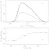 |
Fig. 4 a) Occurrence of wavelet power of velocities vs. normalised broadband intensity Ibb(t − 77.5 s) / Ibb,av at five time steps earlier than the measurement of the velocities. Solid: in period range 150–190 s, dashed: in range 110–150 s, dash-dotted: in range 30–110 s. b) Ratio of power above GR to that above IGR. |
We give in Fig. 4 the dependence of short-period power in the line minimum velocities on the granular convection. Figure 4a) depicts the counts of wavelet power in the period ranges 30–110 s, 110–150 s, and 150–190 s vs. the normalised broadband intensity at each position in the FOV. The broadband images were taken five time steps (=77.5 s) earlier than the wavelet powers. This time lag corresponds approximately to the travel time from the bottom of the photosphere to 540 km height. Only those positions in time and space were counted where the power is more than a factor of 0.2 of the maxima in each period band of width ΔU = 20 s.
Figure 4b) shows the ratio R(U) = P(U)GR / P(U)GR of wavelet power above GR, defined here as I(t − 77.5s)bb / Ibb,av > 1, to that above IGR, i.e. where I(t − 77.5s)bb / Ibb,av < 1. The dependence of this ratio on period U tells that 46% of the total observed wavelet power appears above GR at periods ~180 s, while 35% of the power is measured above GR at periods ~40 s. The relative areas for GR and IGR are found to be 0.45 and 0.55, respectively. Higher velocities occur in IGR areas than in GR areas, but not as extremely different as found in Paper I from the Fe i 5576 line analysis (cf. Fig. 7 there).
The ratio R(U) translates into weights wGR and wIGR for the power spectra above GR and IGR as wGR = R / (1 + R) = P(U)GR / P(U)tot and wIGR = 1 / (1 + R) = P(U)IGR / P(U)tot, respectively. Here, P(U)tot is the total power averaged over the FOV. These weights are to be applied to the total measured power spectrum. We transfer these weights for calculating of power spectra when adopting the (admittedly extreme) cases of GR and IGR models and their atmospheric transmissions from the numerical simulations.
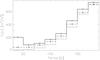 |
Fig. 5 Power of line minimum velocity as function of period with appropriate weights for GR and IGR; thin solid: GR spectrum uncorrected for atmospheric transmission; thick solid and rhombs: GR corrected for transmission; thin dashed: IGR power spectrum uncorrected; thick dashed and asterisks: corrected. |
Figure 5 thus presents the velocity power spectra, dependent on period U, from the wavelet analysis. The power spectra uncorrected for atmospheric transmission and accounting for the transmissions in the GR and IGR model are shown.
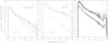 |
Fig. 6 Acoustic energy-flux spectra Fac(ν) from the velocity power spectra assuming an IGR and GR structure from numerical simulation with different densities for IGR and GR; a) and b) for adopted inclination of wave vector vs. vertical θ = 0°; a) for the IGR, dashed: original spectra, solid: corrected for the atmospheric transmission, dash-dotted: from the original power spectrum without high-pass filtering, dotted straight line: adopted frequency dependence for extrapolation; b) for the GR, as a) but without flux from original power spectrum; c) comparison of flux spectra for θ = 0° (thin curves), 30° (medium), and 45° (thick), solid: from GR model, dashed: from the IGR model. |
From the velocity power in Fig. 5, we obtain the total acoustic flux from the wavelet analysis by
![Mathematical equation: \begin{equation} F_\mathrm{ac,tot} = {\rho\over A}\sum_i \left\{\frac{\left[\upsilon_\mathrm{{\rm gr},z}(U_i)\cdot w(U_i)\cdot P_\upsilon(U_i)\right]} {\left[\cos^2(\psi(U_i))\cdot TF(U_i)\right]}\times\Delta U_i\right\} \label{eq11} \end{equation}](/articles/aa/full_html/2010/14/aa14052-10/aa14052-10-eq98.png) (11)
(11)
with ρ = mass density from the GR or IGR models, A = relative area of GR or IGR, w(Ui) = appropriate weights, Pυ(Ui) = measured average power spectrum, and ΔUi = period interval. The correction for inclined particle motion, i.e. 1/cos2ψ, and the transfer function TF(ν) are also included here. The resulting fluxes for GR and IGR are given below in Table 1.
As seen from the Fourier analysis below, the fluxes estimated for adopted inclinations θ of 0°, 30°, and 45° do not differ much. We thus refrain from presenting results of the wavelet analysis for an inclined propagation, especially since the wavelet analysis finds less power than the Fourier analysis at short periods (U = 40–100 s) where the influence of the inclination is least, but where the contribution to the total power is less than from longer periods.
4.2. Fourier analysis
The temporal power spectra were calculated at each pixel and averaged over the FOV. Figure 6 shows the acoustic flux spectra, per mHz, after subtraction of the noise level in the velocity power spectrum. Figures 4a) and b) give the flux spectra when assuming the IGR and the GR model, respectively, for an adopted vertical propagation. The GR flux spectrum is larger than from the IGR model, for two reasons. 1) The density is higher in the GR than in the IGR by approximately a factor of 2.5. 2) The correction for atmospheric transmission is much more in GR than in IGR. It amounts to two orders of magnitude in the 25–30 mHz range for the GR model, while it is only a factor of 5–10 for the IGR model. These two factors accounting for larger flux in GR than in IGR are compensated by a small amount due to the different weights applied to the GR and IGR spectra, cf. Fig 4b) above. Figure 6a) also depicts the flux spectrum for the case without high-pass filtering (cf. end of Sect. 2). Obviously, the flux is larger, and noisier, at all frequencies in this case than with filtering.
Figure 6 indicates the frequency dependences of the acoustic flux spectra. We may extrapolate to higher frequencies and estimate the energy flux carried by acoustic waves with periods U < 40 s (cf. Table 1 below).
Figure 6c) compares the flux spectra assuming both the GR and IGR model for adopted inclinations θ of the wave vector vs. the vertical direction of 0° (thin curves), 30° (medium), and 45° (thick). Also here the flux spectra were corrected for their appropriate transmissions from GR and IGR models. The largest difference is seen at high frequencies for the adopted GR model because here the difference in the transmissions is greatest (see Fig 3); otherwise, the differences are small. The reason comes from several effects that partly compensate for each other. For inclinations of 30° and 45° and at high frequencies, the reduction of the vertical group velocity υgr,z ∝ cosθ and of the increase in the transmission for inclined propagation are partly balanced by the increase in the correction for the squared particle velocity | V | 2 = | Vz | 2 / cos2ψ (cf. Eq. (10)). Near the cutoff frequency and after adopting inclined wave vectors, the fluxes are even larger, though not much, than for vertical wave propagation. There the transmissions are very independent of inclination ~1, the vertical group velocities are υgr,z(θ) ≈ υgr,z(θ = 0°), while cos2ψ < 1.
Adopting inclinations of either 0° or 45° for the whole FOV are extreme assumptions. For a distribution of inclinations over the FOV and over frequency, one should expect a distribution of flux spectra in Fig. 6c) between the limits calculated for the adopted inclinations.
As in Eq. (11), we estimate from the velocity power spectra in Fig. 6 the total acoustic flux from
![Mathematical equation: \begin{equation} F_\mathrm{ac,tot} = {\rho\over A}\sum_k \left\{\frac{\left[\upsilon_\mathrm{{\rm gr},z}(\nu_k)\cdot w(\nu_k)\cdot P_\upsilon(\nu_k)\right]} {\left[\cos^2(\psi(\nu_k))\cdot TF(\nu_k)\right]}\times\Delta\nu_k\right\} , \label{eq12} \end{equation}](/articles/aa/full_html/2010/14/aa14052-10/aa14052-10-eq111.png) (12)
(12)
where Δνk are the frequency intervals, w(νk) = w(1 / Uk) with appropriate interpolation from Ui in Eq. (11) to Uk. The flux values are again given in Table 1.
For the estimate of the total flux we add the flux spectra in Eqs. (11) and (12) only to 25 mHz, and estimate the position of the dotted lines for extrapolation only from the low flux values in the 10–20 mHz range. Apart from fluctuations due to noise, the measured flux spectra decrease monotonically from 6 mHz to 25 mHz, independent of the amount of transmission correction. Even applying large corrections for atmospheric transmission, we find no indication, above noise, of large acoustic flux at frequencies > 20 mHz (or periods < 50 s).
4.3. Discussion
Table 1 summarises the results of the acoustic energy flux measurements. Again, θ denotes the adopted angle of inclination of the wave vector with respect to the vertical. The fluxes are summations over the period range 190 s down to 30 s for the wavelet analysis and over 5.2 mHz to 25 mHz for the Fourier analysis. We distinguish between the results from GR and IGR. Only values corrected for atmospheric transmission are quoted. The averages are the fluxes from GR and IGR with weights of 0.45 and 0.55, respectively, according to their relative areas. The values at 250 km are from Bello González et al. (2009b), where summation was performed up to only 20 mHz.
Energy fluxes in acoustic waves Fac in W m2, where values in brackets include fluxes extrapolated to 100 mHz.
The acoustic fluxes obtained from wavelet and Fourier analysis agree within 18% and less. In the present study, the fluxes from the wavelet analysis are smaller than those from the Fourier analysis. The results from Paper I show the opposite and yet there, no distinction between GR and IGR was made. Inspection of the period/frequency dependences of the fluxes shows that the largest differences are in the GR fluxes in the 10–25 mHz range. We speculate that the differences in flux arise for two reasons: 1) The wavelet measurement is more restrictive in the noise treatment. 2) The summation to yield the total fluxes is coarser in the wavelet analysis with its necessarily broad period intervals than in the Fourier analysis. We thus consider the flux differences as a measurement of the errors.
The bracketed values in Table 1 contain the fluxes from extrapolation, i.e. integration over frequencies from 25 mHz to 100 mHz, or over periods from 10 s to 40 s. We stress that the extrapolation is an estimate based on the flux spectra at frequencies < 20 mHz, or periods > 50 s. Comparison between the unbracketed and bracketed values shows that the extrapolation adopted here does not lead to an important contribution to the total flux. As from the analysis of the Fe i 5576 data in Paper I, we find also here that most of the acoustic flux occurs at periods of 100–190 s.
The GR and IGR atmospheres from numerical simulations represent extreme cases. This leads to the large difference between acoustic flux in GR and IGR by a factor 3 to 4. As seen in Fig. 4, the IGR flux spectrum is low and only needs a “mild” correction. The GR spectrum is, after the large correction, very high and admittedly speculative at frequencies > 20 mHz. This is due to the extended height range of formation of the velocity signal in the GR model. In a next step, one should use a distribution between the extremes of granules and intergranules from the numerical simulations. This allows one to obtain corrections for power spectra from intermediate structures and also to apply appropriate weights and relative areas yielding intermediate flux spectra. For a mixture of atmospheres between very bright GRs and very dark IGRs, the average flux spectrum is expected to lie between the extrema of Fig. 6.
The acoustic energy flux at 500–620 km in the quiet solar atmosphere is thus found in the range of 1730–2060 W m-2. This is a factor 1.7 to 2 higher than the value of ~1000 W m-2, which we interpolated from measurements by Straus et al. (2008), in several spectral lines to a height of 500 km. Yet these measurements were obtained with a slit spectrograph without adaptive optics and probably with lower spatial resolution than in the present study, and they were not corrected for atmospheric wave transmission. Remarkably, these authors find a large amount of energy transported by atmospheric gravity waves into the chromosphere, 5000 W m-2 at 500 km.
5. Conclusions
A two-dimensional time series with high spatial and temporal resolution was obtained from the disc centre of the Sun in the Fe i 5434 Å line which is formed at 500–620 km. For interpreting the wave power measured from Doppler shifts at line minimum, propagation into the vertical direction and with inclinations of 30° and 45° was adopted. We used models of a granule (GR) and intergranule (IGR) from a three-dimensional numerical simulation by Asplund et al. (2000). NLTE radiative transfer calculations in Fe i 5434 Å were carried out for these models as in Shchukina & Trujillo Bueno (2001), from which velocity response functions and atmospheric transmissions of the velocity signals were calculated for the GR and IGR. Wavelet and Fourier analyses were performed to obtain the flux spectra in waves with periods shorter than the acoustic cutoff period, adopting both GR and IGR. We summarise the results here.
-
1.
Assuming the GR model, the acoustic wave flux leads to ~3100 W m-2, a factor of 3 more than for the IGR model, for which we obtain ~1000 W m-2, because the line is formed at layers with higher densities in the GR than in the IGR and because the correction factor due to atmospheric transmission is larger for the GR than for the IGR.
-
2.
Wavelet and Fourier analysis gave approximately the same total fluxes. Yet the wavelet analysis allows the analysis on the power distribution leading to the finding of fluxes related to the granular pattern. Approximately 40% of the signals are detected above GRs and 60% above IGRs. Using appropriate weights depending on period and relative area, we obtain an average power of 1730–2060 W m-2, for inclination θ = 0°.
-
3.
The estimates of the total fluxes become larger by 15% when inclined wave propagation of 45° is assumed.
-
4.
Most acoustic flux is found at periods between 100 s and the acoustic cutoff period of ~193 s. Extrapolation of the flux spectra to periods of 10 s gives only negligible contributions.
The acoustic flux found here at heights of 500–620 km falls short, by a factor of 2.5, of covering the radiative losses of 4600 W m-2 calculated by Vernazza et al. (1981) for their model of the average chromosphere. Including radiative losses from the many Fe ii lines in the solar spectrum, Anderson & Athay (1989) gave an energy need of 14 000 W m-2. Possibly, the acoustic energy flux measured in the present study is sufficient to produce on average a warm, internetwork chromosphere that emits a basal radiative flux (Schrijver 1987), together with the flux in atmospheric gravity waves found by Straus et al. (2008). We may thus consider acoustic waves a viable means of transfering energy to the chromosphere and supplying part of the needs for chromospheric radiative losses.
Our flux measurements were based on models of a granule and an intergranule from numerical simulations. The ensuing determination for the atmospheric transmission gave a mild correction for an intergranular model. The correction for the granular model amounts to two orders of magnitude at frequencies of 25–30 mHz. The granular flux spectrum is thus admittedly speculative at these high frequencies. But we consider it the best estimate we can obtain at present, at least at lower frequencies, while we did not use the flux spectra at ν > 25 mHz for determining the above given total flux.
For the estimates of the total acoustic flux, we adopted the linear theory of adiabatic plane waves in an isothermal atmosphere. This limits the applied theoretical background; we however, admitted oblique propagation in the solar atmosphere. Especially the highly spatial and temporal intermittency of the waves, as revealed by our wavelet analysis, demonstrates the generation and propagation of waves in strong inhomogeneities. An animation of the occurrence of wavelet power together in granulation, velocity, and line minimum intensity is presented in Bello González et al. (2010), albeit from Fe i 5576 Å data. In view of this, we consider it an important further step to guide the interpretation of velocity (and intensity) fluctuations in the solar atmosphere by numerical simulations as in Wedemeyer-Böhm et al. (2007), Straus et al. (2008), and Bello González et al. (2009a). One-dimensional calculations with wave spectra in a model atmosphere do not appear sufficient. Ulmschneider et al. (2005) point out that 1D simulations are misleading because shock merging destroys much of the short-period power.
Three-dimensional simulations become feasible with today’s computer facilities and with the codes being developed. Simulations with high temporal and spatial resolution are definitely needed. They should include the production of acoustic waves by the granular convection and their propagation through the inhomogeneous solar photosphere. They will take the lead in interpretations of what is seen in high-resolution observations.
Acknowledgments
NBG acknowledges financial support by the Kiepenheuer-Institut für Sonnenphysik through the Pakt für Forschung und Innovation of the WGL. M.F.S. was supported by the ERASMUS programme of the European Union. F.K. and O.O. thank for Deutsche Forschungsgemeinschaft support through grants KN 152/29-3,4. The Vacuum Tower Telescope is operated by the Kiepenheuer-Institut für Sonnenphysik, Freiburg, and at the Spanish Observatorio del Teide of the Instituto de Astrofísica de Canarias. Wavelet software was provided by C. Torrence and G. Compo, and is available at the URL: http://paos.colorado.edu/research/wavelets
References
- Anderson, L. S., & Athay, R. G. 1989, ApJ, 346, 1010 [NASA ADS] [CrossRef] [Google Scholar]
- Asplund, M., Nordlund, Å., Trampedach, R., Allen de Prieto, C. A., & Stein, F. R. 2000, A&A, 359, 729 [NASA ADS] [Google Scholar]
- Bello González, N., & Kneer, F. 2008, A&A, 480, 265 [NASA ADS] [CrossRef] [EDP Sciences] [Google Scholar]
- Bello González, N., Okunev, O. V., Domínguez Cerdeña, I., Kneer, F., & Puschmann, K. G. 2005, A&A, 434, 317 [NASA ADS] [CrossRef] [EDP Sciences] [Google Scholar]
- Bello González, N., Yelles Chaouche, L., Okunev, O., & Kneer, F. 2009a, A&A, 494, 1091 [NASA ADS] [CrossRef] [EDP Sciences] [Google Scholar]
- Bello González, N., Flores Soriano, M., Kneer, F., & Okunev, O. 2009b, A&A, 508, 941 (Paper I) [NASA ADS] [CrossRef] [EDP Sciences] [Google Scholar]
- Bello González, N., Flores Soriano, M., Kneer, F., & Okunev, O. 2010, Mem. S.A.It., in press [Google Scholar]
- Bray, R. J., & Loughhead, R. E. 1974, The Solar Chromosphere (New York: John Wiley and Sons, Inc.) [Google Scholar]
- Carlsson, M., Hansteen, V. H., De Pontieu, B., et al. 2007, PASJ, 59, 663 [NASA ADS] [CrossRef] [Google Scholar]
- de Boer, C. R. 1996, A&AS, 120, 195 [Google Scholar]
- Deubner, F.-L. 1976, A&A, 51, 189 [NASA ADS] [Google Scholar]
- Deubner, F.-L., & Fleck, B. 1990, A&A, 228, 506 [NASA ADS] [Google Scholar]
- Eibe, M. T., Mein, P., Roudier, Th., & Faurobert, M. 2001, A&A, 371, 1128 [NASA ADS] [CrossRef] [EDP Sciences] [Google Scholar]
- Fossum, A., & Carlsson, M. 2006, ApJ, 646, 579 [NASA ADS] [CrossRef] [Google Scholar]
- Mein, N., & Schmieder, B. 1981, A&A, 97, 310 [NASA ADS] [Google Scholar]
- Mihalas, B. W., & Toomre, J. 1982, ApJ, 263, 386 [NASA ADS] [CrossRef] [Google Scholar]
- Puschmann, K. G., Kneer, F., Seelemann, T., & Wittmann, A. D. 2006, A&A, 445, 337 [NASA ADS] [CrossRef] [EDP Sciences] [Google Scholar]
- Schrijver, C. J. 1987, A&A, 172, 111 [NASA ADS] [Google Scholar]
- Shchukina, N., & Trujillo Bueno, J. 2001, ApJ, 550, 970 [NASA ADS] [CrossRef] [Google Scholar]
- Straus, T., Fleck, B., Jefferies, S. M., et al. 2008, ApJ, 681, L125 [Google Scholar]
- Torrence, C., & Compo, G. P. 1998, Bull. Amer. Meteor. Soc., 79, 61 [CrossRef] [Google Scholar]
- Ulmschneider, P., Rammacher, W., Musielak, Z. E., & Kalkofen, W. 2005, ApJ, 631, L155 [NASA ADS] [CrossRef] [Google Scholar]
- Vernazza, J. E., Avrett, E. H., & Loeser, R. 1981, ApJS, 45, 635 [NASA ADS] [CrossRef] [Google Scholar]
- von der Lühe, O., Soltau, D., Berkefeld, T., & Schelenz, T. 2003, SPIE, 4853, 187 [Google Scholar]
- Wedemeyer-Böhm, S., Steiner, O., Bruls, J., & Rammacher, W. 2007, in The Physics of Chromospheric Plasmas, ed. I. Dorotovic, P. Heinzel, & R. Rutten, ASP Conf. Ser., 368, 93 [Google Scholar]
All Tables
Energy fluxes in acoustic waves Fac in W m2, where values in brackets include fluxes extrapolated to 100 mHz.
All Figures
|
Fig. 1 Fe i 5434 Å profiles for the atmospheres from numerical simulations by Asplund et al. (2000). The solid line and rhombs: from granule (GR) with infinite spectral resolution and after convolving with FPI spectrometer curve and Hamming smoothing, respectively; dashed and asterisks: the same for intergranular (IGR) area; crosses: average observed profile scaled to the average of the calculated intensities in the wings. |
| In the text | |
|
Fig. 2 Response functions for velocity RFυ(z) from line minimum of Fe i 5434. Dotted line: for IGR with infinite spectral resolution; solid and dashed: for GR and IGR, respectively, after convolution of line profiles with spectrometer function and Hamming function; thick solid: boxcar smoothing of thin (GR) response function over three height positions. |
| In the text | |
|
Fig. 3 Transmission of waves as function of wave period; a) with infinite spectral resolution for IGR (dotted) and after applying the convolution with spectrometer function and filtering; solid: for GR, dashed: for IGR; thin: for waves with amplitudes independent of height, thick: for waves with exponentially increasing amplitude; b) comparison of transmission for waves with exponentially increasing amplitude and with adopted inclination θ of 0°, 30°, and 45°; solid: GR, dashed: IGR. |
| In the text | |
|
Fig. 4 a) Occurrence of wavelet power of velocities vs. normalised broadband intensity Ibb(t − 77.5 s) / Ibb,av at five time steps earlier than the measurement of the velocities. Solid: in period range 150–190 s, dashed: in range 110–150 s, dash-dotted: in range 30–110 s. b) Ratio of power above GR to that above IGR. |
| In the text | |
|
Fig. 5 Power of line minimum velocity as function of period with appropriate weights for GR and IGR; thin solid: GR spectrum uncorrected for atmospheric transmission; thick solid and rhombs: GR corrected for transmission; thin dashed: IGR power spectrum uncorrected; thick dashed and asterisks: corrected. |
| In the text | |
|
Fig. 6 Acoustic energy-flux spectra Fac(ν) from the velocity power spectra assuming an IGR and GR structure from numerical simulation with different densities for IGR and GR; a) and b) for adopted inclination of wave vector vs. vertical θ = 0°; a) for the IGR, dashed: original spectra, solid: corrected for the atmospheric transmission, dash-dotted: from the original power spectrum without high-pass filtering, dotted straight line: adopted frequency dependence for extrapolation; b) for the GR, as a) but without flux from original power spectrum; c) comparison of flux spectra for θ = 0° (thin curves), 30° (medium), and 45° (thick), solid: from GR model, dashed: from the IGR model. |
| In the text | |
Current usage metrics show cumulative count of Article Views (full-text article views including HTML views, PDF and ePub downloads, according to the available data) and Abstracts Views on Vision4Press platform.
Data correspond to usage on the plateform after 2015. The current usage metrics is available 48-96 hours after online publication and is updated daily on week days.
Initial download of the metrics may take a while.