| Issue |
A&A
Volume 521, October 2010
|
|
|---|---|---|
| Article Number | A34 | |
| Number of page(s) | 6 | |
| Section | The Sun | |
| DOI | https://doi.org/10.1051/0004-6361/201014367 | |
| Published online | 18 October 2010 | |
Numerical simulations of the attenuation of the fundamental slow magnetoacoustic standing mode in a gravitationally stratified solar coronal arcade
P. Konkol1 - K. Murawski1 - D. Lee2 - K. Weide2
1 - Group of Astrophysics and Gravity Theory, Institute of Physics, UMCS, ul. Radziszewskiego 10, 20-031 Lublin, Poland
2 -
ASC/Flash Center, The University of Chicago, 5640 S. Ellis Ave, Chicago, IL 60637, USA
Received 5 March 2010 / Accepted 2 June 2010
Abstract
Aims. We aim to explore the influence of thermal conduction
on the attenuation of the fundamental standing slow magnetoacoustic
mode in a two-dimensional (2D) potential arcade that is embedded in a
gravitationally stratified solar corona.
Methods. We numerically solve the time-dependent
magnetohydrodynamic equations to find the spatial and temporal
signatures of the mode.
Results. We find that this mode is strongly attenuated on a time-scale of about 6 waveperiods.
Conclusions. The effect of non-ideal plasma such as thermal
conduction is to enhance the attenuation of slow standing waves. The
numerical results are similar to previous observational data and
theoretical findings for the one-dimensional plasma.
Key words: magnetohydrodynamics (MHD) - Sun: corona - Sun: oscillations
1 Introduction
Observational findings by SUMER SOHO/EIT and TRACE/EUV have revealed that solar coronal plasma is able to sustain (among other waves) both propagating (e.g., De Moortel et al. 2002a,b; Ofman et al. 1997; Murawski & Zaqarashvili 2010) and standing (e.g., Wang et al. 2002) slow magnetoacoustic (slow henceforth for slow magnetoacoustic) waves. Because slow waves are restricted to propagate along magnetic field lines, they are a valuable tool for probing the coronal plasma and providing information within the framework of coronal seismology (e.g., Roberts 2000; Nakariakov & Verwichte 2005; Ballai 2007; Andries et al. 2009).
Slow waves are found to be strongly attenuated over few waveperiods (Wang et al. 2003). Several mechanisms of attenuation of these waves were proposed: wave leakage into the internal layers of the solar atmosphere (Ofman 2002; Van Doorsselaere et al. 2004; Ogrodowczyk & Murawski 2007), lateral wave leakage as a result of the curvature of magnetic field lines (Roberts 2000; Ogrodowczyk et al. 2007), phase mixing (e.g., Ofman & Aschwanden 2002), resonant absorption (Ruderman & Roberts 2002) and non-ideal magnetohydrodynamic (MHD) effects (Roberts 2000; Nakariakov et al. 2000; De Moortel & Hood 2003; Verwichte et al. 2008).
The intensive numerical investigations of slow standing waves in a straight magnetic field topology showed that without large amplitude slow mode oscillations attenuate rapidly due to shock dissipation (Haynes et al. 2008). Fully nonlinear 1D simulations of slow mode oscillations in the presence of thermal conduction were performed by De Moortel & Hood (2003) and Verwichte et al. (2008), who showed that thermal conduction is an important damping mechanism. In particular, De Moortel & Hood (2003) discussed in detail the influence of thermal conduction on slow waves. Their numerical results for driven waves revealed that for typical solar coronal conditions thermal conduction appears to be the dominant wave-attenuation mechanism. Selwa et al. (2005) and Ogrodowczyk & Murawski (2007) showed that pressure pulses triggered near a foot-point excite the fundamental mode. The evolution of standing slow waves in a curved magnetic field topology was discussed by Selwa & Murawski (2006), Selwa et al. (2007a,b 2009), Ogrodowczyk et al. (2007) and Selwa & Ofman (2009) to find that loop curvature leads to the reduction of excitation and attenuation times of slow standing modes in a gravity-free arcade loop.
A study of slow wave propagation in gravitationally stratified media is rare. A theoretical 1D model of propagating slow waves in coronal loops by Nakariakov et al. (2000) includes the effects of stratification, nonlinearity, viscosity, resistivity, and thermal conduction. De Moortel & Hood (2004) investigated the effect of gravitational stratification in a straight magnetic field topology as a mechanism of attenuation of propagating slow waves. In another approach, Mendoza-Briceno et al. (2005) found that in a 1D gravitationally stratified atmosphere the attenuation time of slow standing waves was reduced by 10-20% in comparison to a gravity-free case. Selwa & Ofman (2009) explored slow standing waves in a cold curved, gravitationally stratified loop.
Despite the significant achievements attained in the above mentioned papers there is still a lack of realistic modeling which takes a simultaneous presence of curved magnetic field and gravity into consideration. Although slow propagating waves are an interesting subject to study, we postpone this problem for future studies and limit ourself to slow standing waves. The aim of this paper is to study the influence of thermal conduction on the attenuation of slow standing waves in a gravitationally stratified solar coronal arcade. This way we generalize the model of Verwichte et al. (2008) into a 2D curved geometry and the model of Selwa & Ofman (2009) by inclusion of the photosphere layer, which results in wave reflection. Selwa & Ofman adopted line-tying boundary conditions, which mimic action of the chromosphere/photosphere layer. We also extend the model of De Moortel & Hood (2003), in which damping of slow waves by thermal conduction was studied in the frame of a 1D homogeneous case. We extend their model to a curved magnetic field geometry and 2D case.
This paper is organized as follows. The numerical model is described in Sect. 2. The numerical results are presented in Sect. 3. We concluded with a short summary of the main results in Sect. 4.
2 The numerical model
We performed numerical simulations in a magnetically structured atmosphere. Henceforth, we neglect radiation and plasma heating, viscosity, and resistivity, but take into account isotropic thermal conduction, which is important for the damping of slow waves (Ofman 2002). As a consequence we use the following MHD equations to describe the coronal plasma:

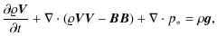
with

Here p* is total (gas plus magnetic) pressure,
Equations (1)-(5) are solved numerically using the new unsplit staggered mesh (USM) MHD solver (Lee & Deane 2009) in FLASH (Fryxell et al. 2000; Dubey et al. 2009). the FLASH architecture is described in Dubey et al. (2009).
The USM solver implements a high-order Godunov scheme in a directionally unsplit formulation,
satisfying the
![]() condition to machine accuracy, using a constrained transport approach
(Evans & Hawley 1988) on a uniform grid as well as the adaptive mesh refinement (AMR) grid.
The USM solver can adopt various types of algorithms that provide first, second, and third order accurate
Riemann reconstructions, different choices for slope limiters and Riemann solvers.
In FLASH, the AMR grid is adopted, using the PARAMESH package (MacNeice et al. 1999).
condition to machine accuracy, using a constrained transport approach
(Evans & Hawley 1988) on a uniform grid as well as the adaptive mesh refinement (AMR) grid.
The USM solver can adopt various types of algorithms that provide first, second, and third order accurate
Riemann reconstructions, different choices for slope limiters and Riemann solvers.
In FLASH, the AMR grid is adopted, using the PARAMESH package (MacNeice et al. 1999).
We use a second-order MUSCL-Hancock method (Toro 1997)
with monotonized central slope limiter and
the HLLD Riemann solver (Miyoshi & Kusano 2005).
We set the simulation box as
![]() and impose fixed-in-time boundary conditions for all plasma quantities in the x- and y-directions, while
all plasma quantities remain invariant along the z-direction.
In our studies we use the AMR grid with a minimum (maximum) level of
refinement set to 4 (6), where each block contains
and impose fixed-in-time boundary conditions for all plasma quantities in the x- and y-directions, while
all plasma quantities remain invariant along the z-direction.
In our studies we use the AMR grid with a minimum (maximum) level of
refinement set to 4 (6), where each block contains
![]() interior cells.
The refinement strategy is based on controlling numerical errors in mass density.
This results in an excellent resolution of steep spatial profiles and greatly reduces numerical diffusion at
these locations.
interior cells.
The refinement strategy is based on controlling numerical errors in mass density.
This results in an excellent resolution of steep spatial profiles and greatly reduces numerical diffusion at
these locations.
2.1 Initial setup
In this section, we detail the initial setup used in this paper. The solar corona is modeled as a low mass density, highly magnetized plasma overlaying a dense photosphere/chromosphere.
2.1.1 The structure of the solar atmosphere
We assume that the solar atmosphere is settled in a two-dimensional
and still (
![]() )
environment. Thus,
we assume that
the pressure gradient force is balanced by the gravity, that is
)
environment. Thus,
we assume that
the pressure gradient force is balanced by the gravity, that is
and the magnetic field is force-free
Here the subscript
Using the ideal gas law and the y-component of the hydrostatic pressure
balance indicated by Eq. (10), we express the background
gas pressure and mass density as
Here
is the pressure scale-height, and
We adopt a smoothed step-function profile for the plasma temperature
![\begin{displaymath}
T_{\rm b}(y) = \frac{1}{2} T_{\rm c} \left[1 + d_{\rm t} +
...
...{\rm tanh} \left(\frac{y-y_{\rm t}}{y_{\rm w}}\right) \right],
\end{displaymath}](/articles/aa/full_html/2010/13/aa14367-10/img42.png)
where
|
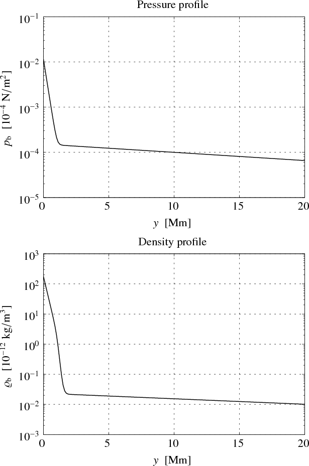
Figure 1: Vertical profiles of a background gas pressure (top panel) and a background mass density (bottom). |
| Open with DEXTER | |
We adopt the magnetic field model was originally described by Priest (1982).
In this model, we assume that Eq. (11) is satisfied by a current-free magnetic field
so that
Here A denotes the magnetic flux function
The background magnetic field components
![\begin{displaymath}(B_{\rm bx},B_{\rm by}) = B_{\rm0} \left[-\cos({x}/{\Lambda}_...
..._{\rm B})\right]
{\rm exp}[-(y-y_{\rm r})/{\Lambda}_{\rm B}] ,
\end{displaymath}](/articles/aa/full_html/2010/13/aa14367-10/img55.png)
in addition to
|
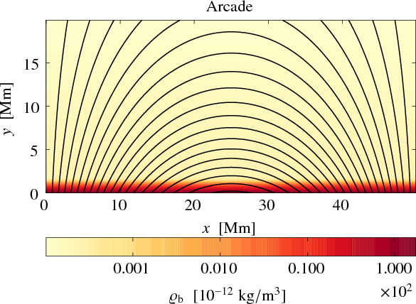
Figure 2: Initial setup of the system. Magnetic lines are represented by solid lines. The mass density is displayed by a color bar. |
| Open with DEXTER | |
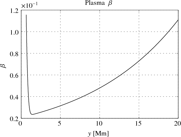
|
Figure 3:
Vertical profile of plasma |
| Open with DEXTER | |
The choice of magnetic field results in the plasma ![]() ,
,

The plasma
2.1.2 Perturbations
Aim to study impulsively excited slow oscillations in the coronal arcade
that is described above. We found that these oscillations are triggered
most effectively by a simultaneous launching of initial pulses in gas pressure
and mass density
with
![$\displaystyle \exp{
\left[
-\frac{(x-x_{\rm0})^2+(y-y_{\rm0})^2}{2w^2}
\right]
}$](/articles/aa/full_html/2010/13/aa14367-10/img70.png)
Here
Unless otherwise stated we set
Figure 3 shows vertical profile of plasma ![]() .
As a result of this background and pulse the resulting standing wave
will move along the magnetic line s with the mean value of
.
As a result of this background and pulse the resulting standing wave
will move along the magnetic line s with the mean value of
![]() .
.
3 Numerical results
The initial pulses of Eqs. (19) and (20) trigger magnetosonic waves. Fast waves propagate essentially isotropically and after a while they leave the simulation region. As slow waves are guided along magnetic field lines, they remain trapped in the system after experiencing reflections from the dense plasma regions.
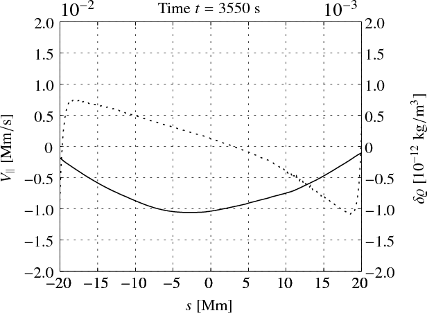
Figure 4 displays a velocity component that is parallel to the magnetic field line,
![]() (solid line), and a mass density
(solid line), and a mass density ![]() (dashed line) at t=3550 s.
Here s denotes the coordinate along the magnetic field line which corresponds to
the magnetic flux function
(dashed line) at t=3550 s.
Here s denotes the coordinate along the magnetic field line which corresponds to
the magnetic flux function
![]() ,
with s=0 denoting the arcade apex.
Note that
,
with s=0 denoting the arcade apex.
Note that
![]() and
and ![]() consist a typical structure for the standing slow mode
(e.g., Nakariakov & Verwichte 2005). The asymmetry in these profiles results
from the strong initial pulse, which significantly perturbes the background state.
consist a typical structure for the standing slow mode
(e.g., Nakariakov & Verwichte 2005). The asymmetry in these profiles results
from the strong initial pulse, which significantly perturbes the background state.
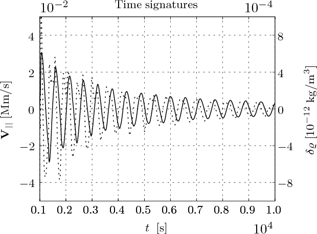
Figure 5 shows the time-signatures that are drawn by collecting wave signals in
![]() and
and ![]() at the detection point (
at the detection point (
![]() Mm,
Mm,
![]() Mm).
These time-signatures reveal oscillations that decay with time and exhibit
the quarter waveperiod phase shift between
Mm).
These time-signatures reveal oscillations that decay with time and exhibit
the quarter waveperiod phase shift between
![]() and
and ![]() ,
which is characteristic
for standing slow waves (Nakariakov & Verwichte 2005;
Ogrodowczyk et al. 2009; Selwa et al. 2005).
,
which is characteristic
for standing slow waves (Nakariakov & Verwichte 2005;
Ogrodowczyk et al. 2009; Selwa et al. 2005).
|
Figure 4: Velocity (solid line) and mass density (dashed line) profiles along the magnetic line. |
| Open with DEXTER | |
|
Figure 5:
Time-signatures of a parallel velocity V|| (solid line) and perturbed mass density (dashed line),
collected at the detection point
|
| Open with DEXTER | |
We estimate the waveperiod P and attenuation time ![]() of the
oscillation by fitting the following attenuated sine function:
of the
oscillation by fitting the following attenuated sine function:
to the time-signatures of Fig. 5. In this case, the waveperiod of the fundamental slow mode can be estimated as
where
|
Figure 6:
Attenuation time |
| Open with DEXTER | |
|
Figure 7:
Ratio of attenuation time |
| Open with DEXTER | |
|
Figure 8:
Ratio of the attenuation time |
| Open with DEXTER | |
|
Figure 9:
Ratio of attenuation time |
| Open with DEXTER | |
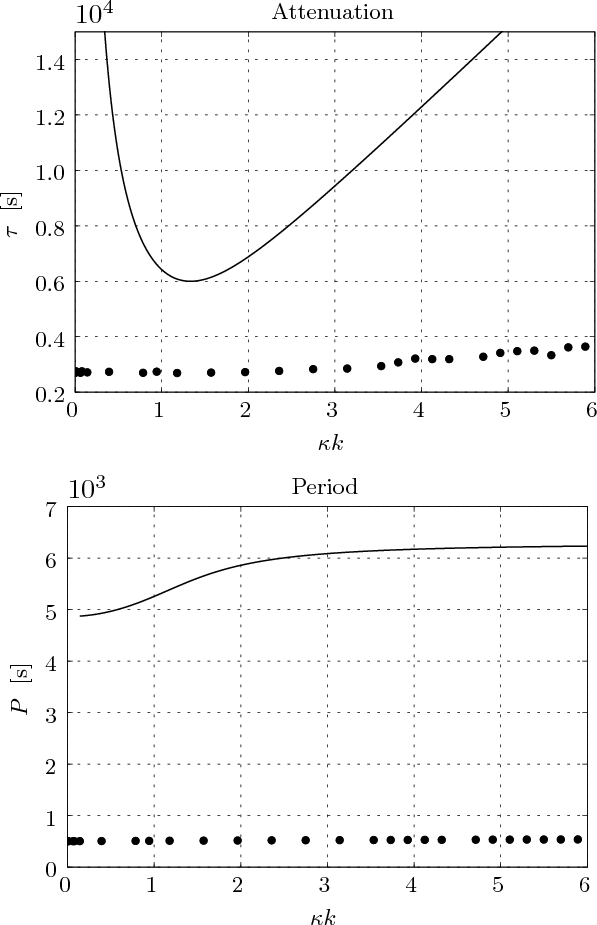
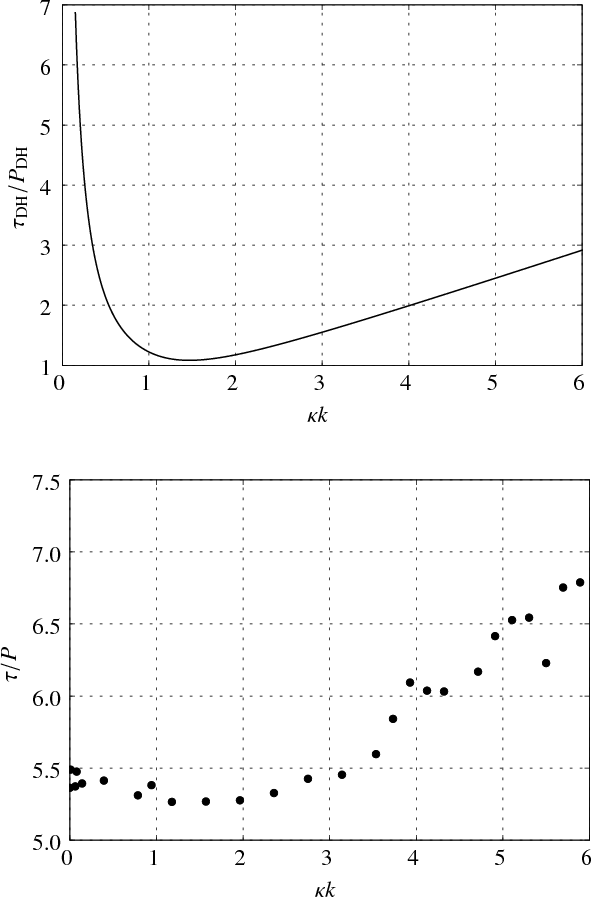
Figure 6 illustrates the attenuation time (top panel) and waveperiod (bottom panel).
The solid lines result from the dispersion relation of
De Moortel & Hood (2003).
From their dispersion relation for a real value of k we obtain a complex wavefrequency
![]() .
Hence we get a wave period
.
Hence we get a wave period
![]() and
attenuation time
and
attenuation time
![]()
The index
Note that De Moortel & Hood (2003) deal with the homogeneous plasma and a straight magnetic field case, while we treat a more complex system in which the fundamental mode is attenuated by thermal conduction as well as by the curved magnetic field (Ogrodowczyk & Murawski 2007; Ogrodowczyk et al. 2009).
In numerical solutions waves are attenuated much stronger than in the theoretical model
of De Moortel & Hood (2003).
This is mainly due to the curved magnetic field, gravity, and non-ideal reflections from
the denser part of the atmosphere.
Those effects are always present, so we have some finite attenuation even for ![]() .
.
The shorter waveperiod in the numerical simulations results from the action of gravity.
For a strictly vertical oscillation the dispersion relation can be written as

where
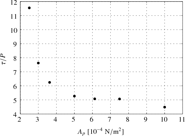
In order to show that these effects are present we ran a few cases for different
values of the sound speed, ![]() .
Note that according to Eq. (14) a higher value of
.
Note that according to Eq. (14) a higher value of ![]() corresponds
to higher
corresponds
to higher ![]() ,
which in turn results in a less inhomogeneous medium.
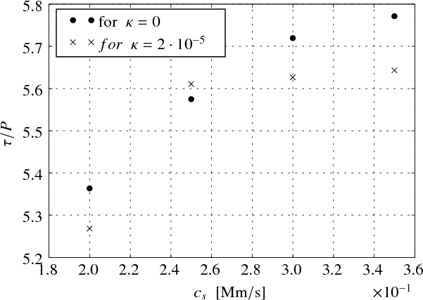
Figure 8 illustrates a dependence of
,
which in turn results in a less inhomogeneous medium.
Figure 8 illustrates a dependence of ![]() on
on ![]() .
As
.
As ![]() grows with
grows with ![]() we infer that for a larger
we infer that for a larger ![]() waves are less attenuated,
which partially explains difference between our results of Fig. 6
for
waves are less attenuated,
which partially explains difference between our results of Fig. 6
for ![]() and those of De Moortel & Hood (2003).
and those of De Moortel & Hood (2003).
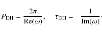
Figure 9 illustrates a dependence of the ratio of attenuation time ![]() and waveperiod P on the initial pulse strength
and waveperiod P on the initial pulse strength ![]() .
According to our expectations
.
According to our expectations ![]() declines with
declines with ![]() ;
for a higher value of
;
for a higher value of ![]() nonlinear effects become more important, which leads to wave steepening.
As a result thermal conduction is more effective for steep profiles,
which explains the fall, off of
nonlinear effects become more important, which leads to wave steepening.
As a result thermal conduction is more effective for steep profiles,
which explains the fall, off of ![]() with
with ![]() (Verwichte et al. 2008).
(Verwichte et al. 2008).
4 Summary
We developed a two-dimensional model of a coronal arcade to explore the attenuation of the fundamental slow magnetoacoustic standing mode in the presence of gravity and thermal conduction.
Our findings can be summarized as follows: the fundamental mode is excited impulsively by localized pulses in gas pressure and mass density that are initially launched in two nearby regions close to the chromosphere/photosphere. The obtained values of attenuation time depart from the analytical data for a homogeneous plasma studied by De Moortel & Hood (2003). This departure results from the adopted model, which implements wave energy leakage as a consequence of curved magnetic field lines and a presence of dense chromosphere/photosphere layer. However, what remains similar in both cases is the existence of some minimal value of damping time for a given wavelength andthermal conductivity. This minimum remains at about the same place.
AcknowledgementsP.K.'s and K.M.'s work was supported by a grant from the State Committee for Scientific Research Republic of Poland, with MNiI grant for years 2007-2010. The software used in this work was in part developed by the DOE-supported ASC/Alliance Center for Astrophysical Thermonuclear Flashes at the University of Chicago.
References
- Andries, J., van Doorsselaere, T., Roberts, B., et al. 2009, Space Sci. Rev., 149, 3 [NASA ADS] [CrossRef] [Google Scholar]
- Ballai, I. 2007, Sol. Phys., 246, 177 [NASA ADS] [CrossRef] [Google Scholar]
- De Moortel, I., & Hood, A. W. 2003, A&A, 408, 755 [NASA ADS] [CrossRef] [EDP Sciences] [Google Scholar]
- De Moortel, I., & Hood, A. W. 2004, A&A, 415, 705 [NASA ADS] [CrossRef] [EDP Sciences] [Google Scholar]
- Dubey, A., et al. 2009, Parallel Computing, accepted [Google Scholar]
- Evans, C. R., & Hawley, J. F. 1988, ApJ, 332, 659 [Google Scholar]
- Fryxell, B., Olson, K., Ricker, P., et al. 2000, ApJS, 131, 273 [NASA ADS] [CrossRef] [Google Scholar]
- Haynes, M., Arber, T. D., & Verwichte, E. 2008, A&A, 479, 235 [NASA ADS] [CrossRef] [EDP Sciences] [Google Scholar]
- Lee, D., & Deane, A. E. 2009, J. Comp. Phys., 228, 952 [Google Scholar]
- MacNeice, P., Olson, K. M., Mobarry, C., de Fainchtein, R., & Packer, C. 1999, CPC, 126, 3 [Google Scholar]
- Mendoza-Briceno, C. A., Erdélyi, R., Sigalotti, L., & Di, G. 2005, ApJ, 624, 1080 [NASA ADS] [CrossRef] [Google Scholar]
- Miyagoshi, T., & Kusano, K. 2005, J. Comput. Phys., 208, 315 [NASA ADS] [CrossRef] [Google Scholar]
- Murawski, K., & Zaqarashvili, T. V. 2010, A&A, accepted [Google Scholar]
- Nakariakov, V. M., Verwichte, E., Berghmans, D., & Robbrecht, E. 2000, A&A, 362, 1151 [NASA ADS] [Google Scholar]
- Nakariakov, V. M., & Verwichte, E. 2005, Living Rev. Sol. Phys., 2, 3 [NASA ADS] [CrossRef] [Google Scholar]
- Ofman, L. 2002, ApJ, 568, L135 [NASA ADS] [CrossRef] [Google Scholar]
- Ofman, L., & Aschwanden, M. 2002, ApJ, 576, L153 [NASA ADS] [CrossRef] [Google Scholar]
- Ofman, L., Romoli, M., Poletto, G., Noci, C., & Kohl, J. I. 1997, ApJ, 491, L111 [NASA ADS] [CrossRef] [Google Scholar]
- Ogrodowczyk, R., & Murawski, K. 2007, A&A, 467, 311 [NASA ADS] [CrossRef] [EDP Sciences] [Google Scholar]
- Ogrodowczyk, R., Murawski, K., & Solanki, S. K. 2009, A&A, 495, 313 [NASA ADS] [CrossRef] [EDP Sciences] [Google Scholar]
- Priest, E. R. 1982, Solar Magnetohydrodynamics (Dordrecht: D. Reidel) [Google Scholar]
- Roberts, B. 2000, Sol. Phys., 193, 139 [NASA ADS] [CrossRef] [Google Scholar]
- Ruderman, M. S., & Roberts, B. 2002, ApJ, 577, 475 [NASA ADS] [CrossRef] [Google Scholar]
- Selwa, M., & Ofman, L. 2009, Ann. Geophys., 27, 3899 [Google Scholar]
- Selwa, M., Murawski, K., & Solanki, S. K. 2005, A&A, 435, 701 [NASA ADS] [CrossRef] [EDP Sciences] [Google Scholar]
- Selwa, M., Ofman, L., & Murawski, K. 2007a, ApJ, 668, L83 [NASA ADS] [CrossRef] [Google Scholar]
- Selwa, M., Murawski, K., Solanki, S. K., & Wang, T. J. 2007b, A&A, 462, 1127 [NASA ADS] [CrossRef] [EDP Sciences] [Google Scholar]
- Toro, E. 1999, Riemann solvers and numerical methods for fluid dynamics (Springer) [Google Scholar]
- Van Doorsselaere, T., Debosscher, A., Andries, J., & Poedts, S. 2004, A&A, 424, 1065 [NASA ADS] [CrossRef] [EDP Sciences] [Google Scholar]
- Verwichte, E., Haynes, M., Arber, T. D., & Brady, C. S. 2008, ApJ, 685, 1286 [NASA ADS] [CrossRef] [Google Scholar]
- Wang, T. J., Solanki, S. K., Curdt, W., Innes, D. E., & Dammasch, I. E. 2002, A&A, 188, 199 [Google Scholar]
- Wang, T. J., Solanki, S. K., Innes, D. E., Curdt, W., & Marsch, E. 2003, A&A, 402, L17 [NASA ADS] [CrossRef] [EDP Sciences] [Google Scholar]
All Figures
|
|
Figure 1: Vertical profiles of a background gas pressure (top panel) and a background mass density (bottom). |
| Open with DEXTER | |
| In the text | |
|
|
Figure 2: Initial setup of the system. Magnetic lines are represented by solid lines. The mass density is displayed by a color bar. |
| Open with DEXTER | |
| In the text | |
|
|
Figure 3:
Vertical profile of plasma |
| Open with DEXTER | |
| In the text | |
|
|
Figure 4: Velocity (solid line) and mass density (dashed line) profiles along the magnetic line. |
| Open with DEXTER | |
| In the text | |
|
|
Figure 5:
Time-signatures of a parallel velocity V|| (solid line) and perturbed mass density (dashed line),
collected at the detection point
|
| Open with DEXTER | |
| In the text | |
|
|
Figure 6:
Attenuation time |
| Open with DEXTER | |
| In the text | |
|
|
Figure 7:
Ratio of attenuation time |
| Open with DEXTER | |
| In the text | |
|
|
Figure 8:
Ratio of the attenuation time |
| Open with DEXTER | |
| In the text | |
|
|
Figure 9:
Ratio of attenuation time |
| Open with DEXTER | |
| In the text | |
Copyright ESO 2010
Current usage metrics show cumulative count of Article Views (full-text article views including HTML views, PDF and ePub downloads, according to the available data) and Abstracts Views on Vision4Press platform.
Data correspond to usage on the plateform after 2015. The current usage metrics is available 48-96 hours after online publication and is updated daily on week days.
Initial download of the metrics may take a while.