| Issue |
A&A
Volume 520, September-October 2010
|
|
|---|---|---|
| Article Number | A105 | |
| Number of page(s) | 8 | |
| Section | The Sun | |
| DOI | https://doi.org/10.1051/0004-6361/201014964 | |
| Published online | 11 October 2010 | |
Scaling of particle acceleration in 3D reconnection at null points
P. K. Browning1 - S. Dalla1,2 - D. Peters1 - J. Smith1
1 - Jodrell Bank Centre for Astrophysics, School of Physics and Astronomy, University of Manchester,
Manchester M13 9PL, UK
2 - Jeremiah Horrocks Institute, University of Central
Lancashire, Preston PR1 2HE, UK
Received 10 May 2010 / Accepted 9 July 2010
Abstract
Context. The strong electric fields associated with magnetic
reconnection are likely to be responsible for the presence of high
energy protons and electrons observed in solar flares. There is much
evidence for 3D reconnection in the solar corona, and we discuss
particle acceleration at 3D reconnection sites. The simplest
configuration for 3D reconnection is at a 3D null point,
where reconnection can take place in spine and fan modes.
Aims. The aim is to understand the properties of accelerated
particles generated by 3D magnetic reconnection, using a test
particle approach, and thus contribute to understanding the origin of
high energy protons and electrons in solar flares. We analyse the
properties of electrons in the magnetic configuration we previously
used to study protons. In addition, we discuss the dependence of the
particle properties on the parameters of the reconnection, such as
strengths of electric and magnetic fields.
Methods. A theoretical framework is presented which can be used
to interpret particle acceleration at 3D null points, and which
shows how strong acceleration can arise. We also use a test particle
approach to calculate particle trajectories in simple model
3D reconnecting nulls. A modified guiding-centre approach is used
for electrons, whilst the full equation of motion is solved for
protons.
Results. Most particle acceleration takes place when particles
closely approach the spine or fan, and we have derived scalings for the
sizes of the localised regions in which strong acceleration occurs. The
energy spectra of protons and electrons are compared, and it is shown
that the spatial distribution of accelerated electrons differs from
protons. A significant number of trapped, high-energy particles can be
generated, which may be observed as coronal HXR sources. The
effectiveness of acceleration increases with the electric-field
magnitude, and decreases with magnetic-field magnitude.
Conclusions. Both protons and electrons can be effectively
accelerated at 3D reconnecting null points. The particle
properties depend on the geometry and field parameters, so that, in
principle, the field configuration may be inferred from observed
properties of particles.
Key words: Sun: particle emission - Sun: X-rays, gamma rays - magnetic reconnection - Sun: flares - Sun: corona
1 Introduction
The role of electric fields associated with magnetic reconnection as accelerators of charged particles is a subject of growing interest. The basic idea is that the strong super-Dreicer electric fields, intrinsic to magnetic reconnection, can directly accelerate charged particles. A major motivation for such studies is to provide an explanation for the large numbers of high energy charged particles inferred from observations of solar flares, particularly in the light of recent observations from RHESSI (e.g. Lin et al. 2003). The presence and properties of accelerated charged particles are also important as a diagnostic of reconnection, since it is virtually impossible to observe the process of reconnection of magnetic field lines in the solar corona directly. Furthermore, magnetic reconnection has been proposed as a particle accelerator in many other contexts: including fusion plasmas (Helander et al. 2002), the Earth's magnetosphere, the heliopause (Lazarian & Opher 2009), microquasars (De Gouevia Dal Pino & Lazarian 2005), pulsars (De Gouevia Dal Pino & Lazarian 2000) and jets in AGNs (Birk et al. 2001). The acceleration of charged particles at magnetic reconnection sites has been widely studied, especially in 2D configurations such as magnetic X points, with and without a ``guide field'', and current sheets (e.g.: Litvinenko 1996; Zharkova & Gordovksyy 2005; Deeg et al. 1991; Vekstein & Browning 1997; Browning & Vekstein 2001; Hannah & Fletcher 2006; Wood & Neukirch 2005). Clearly, such 2D models are highly idealised and 3D configurations are more representative of nature; 3D reconnection is a subject of growing interest, and it is clear that there are distinct qualitative differences between 2D and 3D reconnection (e.g. Birn & Priest 2007).
A natural first step to understanding particle acceleration in the latter is to consider the (arguably) simplest 3D reconnection geometry: a 3D magnetic null point. This is also the most obvious generalisation of the widely-studied 2D X-point. It is becoming clear that 3D null points should be quite ubiquitous in the solar corona; for example, significant numbers of magnetic nulls have been calculated to exist in Quiet Sun fields extrapolated from magnetograms (Longcope & Parnell 2009) and simulations of emerging flux predict a surprisingly large number of null points (Maclean et al. 2009). Several observations of solar flares are suggestive of the presence of reconnection at 3D nulls (Filippov 1999; Aulanier et al. 2000; Fletcher et al. 2001; Des Jardins et al. 2009) and there is also evidence of reconnecting 3D nulls in the Earth's magnetosphere (Xiao et al. 2006). The topology of a 3D null has a spine curve and a fan plane (Lau & Finn 1990), corresponding to the separatrix lines of a 2D X-point. Reconnection may occur in two modes, known as spine or fan reconnection, involving strong current concentrations at the spine or fan, respectively (Priest & Titov 1996).
Particle acceleration in reconnecting fields may be very usefully
studied using the test particle approach, in which the equation of motion
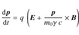
(or its non-relativistic limit) is solved in given background electromagnetic fields
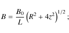
The magnetic field at a simple current-free null is given by
where L is the global field length scale and B0 is the magnetic field strength near the boundary of the reconnection
site (see Fig. 1). The model electric fields investigated, for both spine and fan reconnection are given by
Priest & Titov (1996) (see also Papers I-III for expressions for ![]() ).
Note that the model electromagnetic fields apply only to the outer
``ideal'' reconnection region, and actually diverge as the spine line
or fan plane (according to the mode of reconnection) is approached;
we remove these divergences by applying a cut-off close to the
spine/fan (see Papers I and III). More realistically, the
electromagnetic fields in these localised regions should be calculated
invoking resistivity or other non-ideal effects;
in these regions, particles may also be accelerated directly by
parallel electric fields.
Nevertheless, the volume of these ``dissipation'' regions is very
small, and the proportion of particles reaching them is
thus very low: hence, the energy spectra obtained should be unaffected
by their neglect, except for a few particles in the high energy tail.
).
Note that the model electromagnetic fields apply only to the outer
``ideal'' reconnection region, and actually diverge as the spine line
or fan plane (according to the mode of reconnection) is approached;
we remove these divergences by applying a cut-off close to the
spine/fan (see Papers I and III). More realistically, the
electromagnetic fields in these localised regions should be calculated
invoking resistivity or other non-ideal effects;
in these regions, particles may also be accelerated directly by
parallel electric fields.
Nevertheless, the volume of these ``dissipation'' regions is very
small, and the proportion of particles reaching them is
thus very low: hence, the energy spectra obtained should be unaffected
by their neglect, except for a few particles in the high energy tail.
| Figure 1: The configuration at the 3D null point showing typical fieldlines, the null point, the spine (coinciding with the z axis in the coordinate system used here) and the fan (coinciding with the xy plane). |
|
| Open with DEXTER | |
The global electromagnetic fields are quantified by the strength of the magnetic fields and electric fields at the global scale (the edge of the reconnection region), B0 and E0 respectively, and the typical global length-scale L. Clearly particle behaviour will also depend on the species charge q and mass m; usually, we consider protons or electrons, so q = e. Hitherto, we have presented results for particle acceleration mainly for a single set of parameters for the reconnecting electromagnetic fields, representative of the solar corona. The aim of this paper is to gain an overview of the previous results and to determine the effect of varying the electromagnetic fields, as well as considering different particle species. In previous work, we analysed only protons, but here we will also consider electrons, and investigate the extent to which the efficacy of acceleration is species-dependent.
In Sect. 3 of this paper, we thus consider a population of electrons and calculate their trajectories for the same electromagnetic fields previously used for protons. Numerical integration of electron trajectories is much more demanding than that for protons. This is because the time-scale characterising the electron gyromotion, the electron gyroperiod, is 1837 times smaller than for protons, requiring a much smaller integration time-step than in the proton case. The full orbit approach that we adopted previously, in order to be able correctly to describe particle motion in the dissipation region, becomes prohibitively time-consuming in the case of electrons. For this reason, gyro-averaged equations for particle motion were derived and electron trajectories obtained by integrating them everywhere except in a small region in which the adiabatic description for electrons fails, and the full Lorentz equations are solved.
The purpose of the present paper is to analyse fully how acceleration at a reconnecting 3D null point varies with particle species and with the magnitudes of the governing electromagnetic fields. Although we specifically use the idealised model fields of Priest & Titov (1996), the results should be quite generic. We focus mainly on spine reconnection; however, the scalings will apply equally to fan reconnection, and the differences between spine and fan modes have already been discussed in Paper III. Essentially, this paper completes our study of particle acceleration in the Priest and Titov electromagnetic fields, and provides a very useful framework for undertaking and interpreting test particle studies in more realistic field configurations. In Sect. 2, we consider all the governing variables and relevant dimensionless parameters, and analyse how these are expected to affect the acceleration process. This sets up a theoretical framework for interpretation of our numerical results on particle acceleration at 3D nulls, which is also applicable to more complex and realistic 3D null point model fields. Section 3 considers electron acceleration, and compares this with our previous studies of protons. Numerical results demonstrating the scaling of the particle acceleration process with the parameters of the external fields are presented in Sect. 4. Conclusions are presented in Sect. 5.
2 Parameters and scalings
In order to interpret numerical results on particle orbits, it is very useful first to consider
the relevant dimensionless parameters and how these affect the particle behaviour.
Following Burkhart et al. (1990), Vekstein & Priest (1995) and Vekstein & Browning (1997),
who considered particle acceleration in 2D reconnecting fields, we
can identify two basic parameters which are equally relevant to 3D configurations.
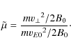
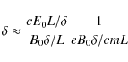
Firstly, the degree of magnetisation at the global scale is quantified by
where

If
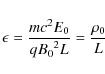
Secondly, the strength of the driving electric field is quantified by the parameter

where
|
(8) |
If the electric drift at global length scales is strong compared with the thermal gyro-motion (
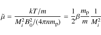
Expressing
![]() ,
where Mi is the magnetic Mach number of the
reconnection inflow and
,
where Mi is the magnetic Mach number of the
reconnection inflow and ![]() is the Alfven speed at global scales, we can also write
is the Alfven speed at global scales, we can also write
|
(9) |
where n is density, T is temperature and

|
(10) |
where
In the case of 2D magnetic null points, it has been shown (e.g. Vekstein & Priest 1995; Burkhart et al. 1990) that the condition of strong magnetisation breaks down in
the vicinity of the X-point, in a region of size
![]() .
This
defines the size of the unmagnetised region, which
arises since the Larmor radius becomes
increasingly large as the magnetic field approaches zero. This limiting length-scale can be derived either by equating
the local gyro-frequency of the particles (
.
This
defines the size of the unmagnetised region, which
arises since the Larmor radius becomes
increasingly large as the magnetic field approaches zero. This limiting length-scale can be derived either by equating
the local gyro-frequency of the particles (
![]() )
to the local electric drift time
(
vE0(r*)/r*), or by equating the
inertial term in the equation of motion to the
electric field acceleration. Within the unmagnetised region, particles
are directly accelerated by the electric field. This may also be
intepreted in terms of the magnitude of the electric field: even the
strong-electric-field guiding-centre theory presented by Northrop (1963) is valid only if the perpendicular electric field is
zeroth-order or less (with reference to the relevant small parameter, which is the dimensionless Larmor radius),
and hence breaks down if
)
to the local electric drift time
(
vE0(r*)/r*), or by equating the
inertial term in the equation of motion to the
electric field acceleration. Within the unmagnetised region, particles
are directly accelerated by the electric field. This may also be
intepreted in terms of the magnitude of the electric field: even the
strong-electric-field guiding-centre theory presented by Northrop (1963) is valid only if the perpendicular electric field is
zeroth-order or less (with reference to the relevant small parameter, which is the dimensionless Larmor radius),
and hence breaks down if ![]() becomes of larger magnitude.
becomes of larger magnitude.
What is the equivalent condition for reconnection at 3D nulls? Whilst
particles can become unmagnetised near the null, as at 2D X-points, due to the
reducing magnetic field strength, they can also become unmagnetised near the spine curve
or fan plane, due to the increasing drift speed.
The spine and fan regimes
must be considered separately. In each case, we define ![]() (corresponding to r* of the 2D case)
to be the length-scale of the unmagnetised region; this is found from the condition
(corresponding to r* of the 2D case)
to be the length-scale of the unmagnetised region; this is found from the condition
where
|
(12) |
here, R is a cylindrical radial coordinate.
For spine reconnection, consider first particles which are approaching the spine (the z axis)
but are still far from the null (
![]() ). Thus
). Thus
![]() while
while
![]() ;
hence
;
hence
![]() .
The condition (11) becomes
.
The condition (11) becomes

|
(13) |
| (14) |
However, if particles approach the null itself (so
|
(15) |
| (16) |
Hence the unmagnetised region is a narrow cylindrical region around the spine, given by
For the fan reconnection regime, the scaling of the electric drift speed is
|
(17) |
Following similar arguments to above, it can be shown that the particles become unmagnetised if they approach the fan plane within a distance

|
(18) |
or within a spherical region around the null, so that the distance from the null is
| (19) |
Particle acceleration can thus happen in two ways. Firstly, as discussed by Vekstein & Browning (1997), the streamline curvature
and non-uniformity of
the
![]() drift can lead to particle acceleration and
gains in parallel velocity, even in the guiding-centre regime. Also,
the curvature and gradient drifts can allow particles to move parallel to the electric field and hence gain energy
(Guo et al. 2010).
This happens to some
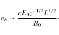
extent in our trajectories. The natural velocity-scale for this is the electric-drift speed
vE0 = cE0/B0, and
we would thus expect velocity gained to scale with this, while the
kinetic energy gain should scale as
drift can lead to particle acceleration and
gains in parallel velocity, even in the guiding-centre regime. Also,
the curvature and gradient drifts can allow particles to move parallel to the electric field and hence gain energy
(Guo et al. 2010).
This happens to some
extent in our trajectories. The natural velocity-scale for this is the electric-drift speed
vE0 = cE0/B0, and
we would thus expect velocity gained to scale with this, while the
kinetic energy gain should scale as
![]() .
It
should be noted, however, that the actual speed acquired by individual particles
may exceed vE by a large factor.
Secondly, when particles reach the unmagnetised regions
(near the spine or fan),
as described above, they are directly accelerated by the electric field until
the weak magnetic field causes them to be ejected from this region.
The strong increase in electric field in 3D null reconnection, as the spine line or fan plane
are approached, means this effect can be very significant. This is illustrated in Fig. 2,
which analyses a typical particle trajectory for spine reconnection
(taken from Paper I) in order to show the origins of the
acceleration.
Note that as the particle approaches the spine, the Larmor radius (
.
It
should be noted, however, that the actual speed acquired by individual particles
may exceed vE by a large factor.
Secondly, when particles reach the unmagnetised regions
(near the spine or fan),
as described above, they are directly accelerated by the electric field until
the weak magnetic field causes them to be ejected from this region.
The strong increase in electric field in 3D null reconnection, as the spine line or fan plane
are approached, means this effect can be very significant. This is illustrated in Fig. 2,
which analyses a typical particle trajectory for spine reconnection
(taken from Paper I) in order to show the origins of the
acceleration.
Note that as the particle approaches the spine, the Larmor radius (![]() )
becomes large, associated with strong increases in
electric field and electric drift-speed. The kinetic energy rises
gradually during the approach, in which the particle is moving adiabatically, but rises sharply in the vicinity of the spine,
as the electric field directly accelerates the particle there. Consideration of the magnetic moment (
)
becomes large, associated with strong increases in
electric field and electric drift-speed. The kinetic energy rises
gradually during the approach, in which the particle is moving adiabatically, but rises sharply in the vicinity of the spine,
as the electric field directly accelerates the particle there. Consideration of the magnetic moment (![]() )
shows that
the motion is approximately adiabatic except near the spine, where there is a jump in magnetic moment.
)
shows that
the motion is approximately adiabatic except near the spine, where there is a jump in magnetic moment.
![\begin{figure}
\par\includegraphics[width=9cm,clip]{14964fg2.ps}
\end{figure}](/articles/aa/full_html/2010/12/aa14964-10/img60.png)
|
Figure 2:
An analysis of the quantities involved in the acceleration of a typical particle in spine reconnection. The standard
field parameters of Papers I and II are used. From top to bottom panels, the quantities displayed are:
distance from the null (r); electric field magnitude (E); Larmor radius ( |
| Open with DEXTER | |
It should
be noted that the simple Priest and Titov fields have unphysical singularities; these
would be resolved in more realistic models which include resistive (or other)
dissipative effects near the spine/fan. However, in a highly conducting plasma the dissipative region will have a
very small size, and the electric fields will still become very large in the outer ideal
region before dropping to zero within the dissipation layer. Consider, for example, the
analytical model fields of Craig & Fabling (1996), which include self-consistently the resistive term in Ohm's law.
The electric field is described by a function which grows to large values as the
radius approaches zero (in spine reconnection), but which then drops smoothly to
zero in a region which scales as
![]() ,
where
,
where ![]() is the resistivity. Particles which arrive close to the spine
or fan (according to the mode of reconnection) may thus be strongly accelerated, and
the overall effectiveness of acceleration is thus determined mainly by the proportion
of particles which reach these strong field regions.
is the resistivity. Particles which arrive close to the spine
or fan (according to the mode of reconnection) may thus be strongly accelerated, and
the overall effectiveness of acceleration is thus determined mainly by the proportion
of particles which reach these strong field regions.
We can interpret the particle trajectories as follows. In the case of spine reconnection,
consider a particle entering in the inflow region in z >0. Initially, the particle
is well modelled by a guiding-centre approach, and it is carried towards the spine
by the electric drift which is in a constant-![]() plane (here
plane (here ![]() is the azimuthal angle) while experiencing weak azimuthal
drifts; thus the dominant velocity components are vr < 0and vz<0. Near the spine, the azimuthal electric field produces a strong
increase in
is the azimuthal angle) while experiencing weak azimuthal
drifts; thus the dominant velocity components are vr < 0and vz<0. Near the spine, the azimuthal electric field produces a strong
increase in ![]() ,
causing the particle to rotate about the spine (gaining kinetic energy
as its potential energy changes - note that, as pointed out in Paper I, potential energy
is proportional to
,
causing the particle to rotate about the spine (gaining kinetic energy
as its potential energy changes - note that, as pointed out in Paper I, potential energy
is proportional to ![]() ). However, the increasing azimuthal speed
builds up a centrifugal radial acceleration term
). However, the increasing azimuthal speed
builds up a centrifugal radial acceleration term
![]() ,
so that vr becomes
positive and the particle is ejected from the vicinity of the spine.
Note that in this case, the energy gain should scale as
,
so that vr becomes
positive and the particle is ejected from the vicinity of the spine.
Note that in this case, the energy gain should scale as
![]() .
.
The analytical results in this section will be used to interpret the numerical results presented in Sect. 4. First, however, we need to produce particle trajectories for electrons (as well as ions, as has been done previously), and this is discussed in the next section.
3 Electron acceleration
Previous test particle results for 3D nulls (Papers I-III) have considered only protons. In principle, the same code
used to calculate proton orbits could also be used
to study electrons; but it is extremely inefficient to solve the full equation of motion
for electrons across the bulk of the region, due to their very small Larmor radius.
In fact, whilst individual trajectories can be calculated in this way, the computer
time required to develop a full spectrum is prohibitively large. A further difference
between electrons and ions is that the former, due to their much smaller rest mass,
often acquire relativistic speeds, whereas the latter can be well-modelled by the
non-relativistic equation of motion. It is thus natural to use a relativistic guiding-centre
approach in order to calculate electron trajectories: the rapid gyromotion is averaged out, appearing
only through the magnetic moment ![]() ,
which is an adiabatic invariant.
It is then required to calculate the parallel and perpendicular (drift) velocities of the
guiding centre. It must be recalled that this approach is valid in the case of small Larmor
radius and large gyro-frequency:
,
which is an adiabatic invariant.
It is then required to calculate the parallel and perpendicular (drift) velocities of the
guiding centre. It must be recalled that this approach is valid in the case of small Larmor
radius and large gyro-frequency:
![]() and
and
![]() where l and Tare the length-scales and time-scale of the background fields (which must be defined
locally, so that l, for example, is not necessarily the same as L).
where l and Tare the length-scales and time-scale of the background fields (which must be defined
locally, so that l, for example, is not necessarily the same as L).
In the case of fast magnetic reconnection, the motion is dominated by the strong electric drift (see Sect. 2). We thus use the guiding-centre equations given by Northrop (1963), which incorporate the strong-electric-drift terms, as previously used to study particle acceleration in 2D reconnecting fields (Vekstein & Browning 1997; Browning & Vekstein 2001; Wood & Neukirch 2005). As mentioned above, we must extend the approach used by these authors by using the full relativistic guiding-centre equations.
However, whilst the guiding-centre approximation is very good on global scales,
we know, as discussed above, that
the Larmor radius becomes large as particles approach the spine; thus the
guiding-centre approximation breaks down and the full equation of motion (1) must be solved. We have therefore developed
a code which switches between the guiding-centre and full equation
of motion as appropriate. The switching condition depends on the
comparison of the Larmor radius and local length-scale, hence on
the local value of
![]() .
By comparing
single particle trajectories for guiding-centre and full-trajectory codes,
we find that, in practice, accurate trajectories are obtained
from the guiding-centre code only if
.
By comparing
single particle trajectories for guiding-centre and full-trajectory codes,
we find that, in practice, accurate trajectories are obtained
from the guiding-centre code only if
![]() is very small. The switching is then determined geometrically,
transitioning to a full-trajectory calculation when the particle approaches either within a certain small
distance from the spine or a larger distance from the null: this
is as predicted in Sect. 2 above, but the exact
length-scales for switching are determined empirically. When a full trajectory
switches to a guiding-centre, we determine the starting
is very small. The switching is then determined geometrically,
transitioning to a full-trajectory calculation when the particle approaches either within a certain small
distance from the spine or a larger distance from the null: this
is as predicted in Sect. 2 above, but the exact
length-scales for switching are determined empirically. When a full trajectory
switches to a guiding-centre, we determine the starting ![]() value - and hence
value - and hence
![]() - by averaging over
several gyro-orbits and subtracting the calculated drift components. The initial
guiding-centre location is obtained also by averaging. Switching back
to a full trajectory code, we use the known values of
- by averaging over
several gyro-orbits and subtracting the calculated drift components. The initial
guiding-centre location is obtained also by averaging. Switching back
to a full trajectory code, we use the known values of ![]() ,
,
![]() and v
and v
![]() ,
along with a randomly-assigned gyro-phase, to specify
the initial cartesian components of
,
along with a randomly-assigned gyro-phase, to specify
the initial cartesian components of ![]() ;
the initial position is determined
by the guiding-centre position with a correction for the known gyro-radius and
randomly assigned gyro-phase. The results have been tested against
full-trajectory simulations, and give very good accuracy but greatly improved
computational time.
;
the initial position is determined
by the guiding-centre position with a correction for the known gyro-radius and
randomly assigned gyro-phase. The results have been tested against
full-trajectory simulations, and give very good accuracy but greatly improved
computational time.
Using this approach, we determine the energy spectrum for a population of
electrons injected randomly in the inflow region of a spherical surface
r = L for the spine reconnection regime. We consider exactly the same electromagnetic fields used
for protons in Paper II, regarded here as the standard condition set:
these are B0 =100 Gauss, E0 = 1.5 kV/m = 0.05 statvolt/cm and scale-length L = 10 km.
Other parameters are also the same as for the proton simulations: thus, we consider a population
of 10 000 electrons with initial velocities randomly distributed according to a Maxwellian with temperature
1 million K (=86 eV).
The results, showing how a steady-state spectrum develops in time,
are shown in Fig. 3. This must be compared
with the proton spectrum (Fig. 2 of Paper II, also reproduced in
Fig. 5 below, left panel) for the same conditions. The
spatial distribution of electrons accelerated to different energies is shown in
Fig. 4,
which again should be compared
with the equivalent proton results (Fig. 3 of Paper II). Note
that in this diagram the spine corresponds to latitudes of ![]()
![]() (and any longitude value) while the fan plane corresponds to zero latitude. The
colour-coding is according to the final
energies of the particles; this shows how the energy gain of a particle
depends on its injection position. However, the dependence of energy
gain on initial position is much less clear for
electrons than for protons (see Papers I and II); this is
because electrons are much more strongly affected by their initial
velocity, as discussed below.
(and any longitude value) while the fan plane corresponds to zero latitude. The
colour-coding is according to the final
energies of the particles; this shows how the energy gain of a particle
depends on its injection position. However, the dependence of energy
gain on initial position is much less clear for
electrons than for protons (see Papers I and II); this is
because electrons are much more strongly affected by their initial
velocity, as discussed below.
An important conclusion is that the 3D reconnection does indeed accelerate electrons quite efficiently. For our chosen field parameters, electrons with energies of up to almost 100 keV are produced, which compares favourably with flare observations. The electrons are less strongly accelerated than the protons - in the sense that the proportion of electrons accelerated is less - but electrons have an overall harder spectrum. The electron energy spectrum shows a fairly distinctive broken-power law shape, with a flatter slope at high energies. This is also consistent with observations.
The times shown in Fig. 3 are normalised with respect to the electron gyro-period. It may be seen that,
in these normalised units, it takes much longer for electrons to establish a steady-state energy spectrum than protons (around
![]() gyro-periods). However, the electron gyro-period is of course much shorter than that for protons: for our chosen standard
conditions, the electron gyro-period is
gyro-periods). However, the electron gyro-period is of course much shorter than that for protons: for our chosen standard
conditions, the electron gyro-period is
![]() s whereas the proton gyro-period is
s whereas the proton gyro-period is
![]() s.
Thus, electrons reach a steady-state in a time of
about 80 ms, which is very similar to the value for protons,
70 ms (see Paper II).
s.
Thus, electrons reach a steady-state in a time of
about 80 ms, which is very similar to the value for protons,
70 ms (see Paper II).
It may also be noted from Fig. 4 that the spatial distribution of the accelerated electrons differs from
that of protons. This means that emission from high energy protons and electrons may be spatially
separated, as also predicted in the case of 2D reconnection with a guide field by Browning & Vekstein (2001)
and Zharkova & Gordovksyy (2005). This is consistent with RHESSI observations (as noted by Zharkova & Gordovksyy 2005). The reasons
for the difference here is associated with the parameter
![]() given by Eq. (7).
The drift speed is the same for protons
and electrons, but (for the same thermal energy)
given by Eq. (7).
The drift speed is the same for protons
and electrons, but (for the same thermal energy) ![]() is different. Hence, for our chosen
parameters, the electrons are actually in the weak-drift regime whereas protons are in the strong-drift
regime, leading to quite different behaviour. The electron spatial distribution seems much less structured,
since the trajectories are far more sensitive to the initial velocity.
is different. Hence, for our chosen
parameters, the electrons are actually in the weak-drift regime whereas protons are in the strong-drift
regime, leading to quite different behaviour. The electron spatial distribution seems much less structured,
since the trajectories are far more sensitive to the initial velocity.
![\begin{figure}
\par\includegraphics[width=9cm,clip]{14964fg3.ps}
\end{figure}](/articles/aa/full_html/2010/12/aa14964-10/img80.png)
|
Figure 3: Time evolution of the energy spectra for electrons in standard conditions. |
| Open with DEXTER | |
![\begin{figure}
\par\includegraphics[width=12cm,clip]{14964fg4.ps}
\end{figure}](/articles/aa/full_html/2010/12/aa14964-10/img81.png)
|
Figure 4: Initial and final positions of electrons, colour-coded according to their final energy. |
| Open with DEXTER | |
![\begin{figure}
\par\includegraphics[width=17cm,clip]{14964fg5.ps}
\end{figure}](/articles/aa/full_html/2010/12/aa14964-10/img82.png)
|
Figure 5: Time evolution of proton spectrum for B=100 Gauss (standard conditions, left) and B=20 Gauss ( right). |
| Open with DEXTER | |
4 The effect of changes in the field magnitudes: numerical results
We now analyse how the parameters of the accelerated population of energetic particles scale if we vary the magnitudes of the electric and magnetic field in our spine reconnection configuration.
In each case, we inject a population of 10 000 protons on random positions in the inflow regions at a distance of L = 10 km from the null, with initial velocities distributed according to a Maxwellian with temperature 106 K; these are followed until a steady-state energy spectrum is achieved.
The first thing to point out is that the acceleration time (
![]() ),
or the time for the energy spectrum to reach
a steady-state, depends on the field magnitudes. The acceleration time
is dominated by the time for the particles to reach the spine due to
the electric drift (when they are near the spine, they gain energy much
more rapidly, as seen in Fig. 2). This scales as
),
or the time for the energy spectrum to reach
a steady-state, depends on the field magnitudes. The acceleration time
is dominated by the time for the particles to reach the spine due to
the electric drift (when they are near the spine, they gain energy much
more rapidly, as seen in Fig. 2). This scales as

|
(20) |
However, in our simulations, time is non-dimensionalised with respect to the gyro-period
Now we consider steady-state energy spectra with varying field magnitudes. As discussed above,
these require following particles for correspondingly varying times
![]() .
Three condition sets are considered:
standard conditions (see above); a factor of 5 decrease in magnetic field (B = 20 Gauss); a factor of 5 increase in electric field (E =
0.025 statvolt/cm).
.
Three condition sets are considered:
standard conditions (see above); a factor of 5 decrease in magnetic field (B = 20 Gauss); a factor of 5 increase in electric field (E =
0.025 statvolt/cm).
The scaling with magnitude of the magnetic field can be partly understood by
considering the electric drift-speed which is
![]() .
Decreasing the
magnitude of the magnetic field results in a more efficient drift of particles
towards the region of strong electric field, and consequently more particles
being accelerated. Conversely, increasing the electric field
enhances the acceleration. It can be seen from Fig. 6
that either increasing electric field or reducing magnetic field increases, overall, the number of non-thermal
particles (this can be best seen by looking at the reduction in the number of low energy, thermal particles).
However, note that with a simple dependence purely on drift-speed, we would expect that increasing
the electric field by a factor of 5 would have the same effect as reducing the magnetic field by the same factor.
It can be seen from Fig. 6
that the situation is more complex than this, and the shape of the
spectra
is quite different. This is probably due to the fact that the
non-adiabatic behaviour, as discussed in Sect. 2, plays
a very significant role, and this is not dependent on the drift-speed.
At stronger electric fields, the energy spectrum has a similar slope,
but generally a larger number of accelerated particles; notably, the
spectrum extends to higher energies, with a fraction of particles
attaining
energies of almost 100 MeV. Reducing the magnetic field leads to a
spectrum which departs significantly from a simple power law
form. The acceleration is enhanced, especially in the intermediate
energy range.
.
Decreasing the
magnitude of the magnetic field results in a more efficient drift of particles
towards the region of strong electric field, and consequently more particles
being accelerated. Conversely, increasing the electric field
enhances the acceleration. It can be seen from Fig. 6
that either increasing electric field or reducing magnetic field increases, overall, the number of non-thermal
particles (this can be best seen by looking at the reduction in the number of low energy, thermal particles).
However, note that with a simple dependence purely on drift-speed, we would expect that increasing
the electric field by a factor of 5 would have the same effect as reducing the magnetic field by the same factor.
It can be seen from Fig. 6
that the situation is more complex than this, and the shape of the
spectra
is quite different. This is probably due to the fact that the
non-adiabatic behaviour, as discussed in Sect. 2, plays
a very significant role, and this is not dependent on the drift-speed.
At stronger electric fields, the energy spectrum has a similar slope,
but generally a larger number of accelerated particles; notably, the
spectrum extends to higher energies, with a fraction of particles
attaining
energies of almost 100 MeV. Reducing the magnetic field leads to a
spectrum which departs significantly from a simple power law
form. The acceleration is enhanced, especially in the intermediate
energy range.
The effect of varying field magnitudes on the spatial distribution of accelerated particles can be seen in
Fig. 7, which shows the injection and final positions of particles, colour-coded according
to their final energies. The case shown has reduced electric field magnitude (by a factor of 1/5) compared with standard
conditions.
This should be compared with Fig. 3
of Paper II. It can be seen clearly that there are no particles in
the highest energy range (>10 MeV). Furthermore, the dependence
of particle energy gain on injection poistion is weaker for the reduced
electric field,
since the initial velocity has relatively more effect. However, it is
still the case that those particles whose injection position
allows them to approach closest to the spine gain the most energy.
The escaping high-energy particles are concentrated, as before, in jets
along the spine (corresponding
to latitudes of close to
![]() ). A considerable population of high-energy particles is also found in the outflow region at
a broad range of latitudes. These form a trapped high-energy population, with particles bouncing in the fieldlines and
only weakly drifting across the field.
). A considerable population of high-energy particles is also found in the outflow region at
a broad range of latitudes. These form a trapped high-energy population, with particles bouncing in the fieldlines and
only weakly drifting across the field.
![\begin{figure}
\par\includegraphics[width=9cm]{14964fg6.ps}
\end{figure}](/articles/aa/full_html/2010/12/aa14964-10/img88.png)
|
Figure 6: The effects of varying electric and magnetic field magnitudes on the steady-state energy spectra. |
| Open with DEXTER | |
![\begin{figure}
\par\includegraphics[width=12cm,clip]{14964fg7.ps}
\end{figure}](/articles/aa/full_html/2010/12/aa14964-10/img90.png)
|
Figure 7:
Particle injection (top) and final (bottom) positions plot for an electric field strength 1/5 of standard (
|
| Open with DEXTER | |
5 Summary and conclusions
We have considered acceleration of charged particles at reconnecting 3D magnetic null points, for spine reconnection, focusing on understanding the acceleration process and how it depends on particle species and on the magnitudes of the underlying electromagnetic fields. Both protons and electrons have been considered, with the development of a new code which switches from guiding-centre to full equation of motion in order to model the latter.
As well as completing the analysis of charged particle acceleration in the idealised model fields of Priest & Titov (1996), we have provided a theoretical framework for interpretation of other studies of particle acceleration at 3D nulls. Acceleration can take place both adiabatically, away from the spine and fan, and non-adiabatically, when the particles can become unmagnetised. In our configuration, the latter process dominates, and we have identified the scalings for the sizes of the regions in which direct electric field acceleration takes place.
We found that electrons are generally less efficiently accelerated than protons, because they are more likely to be in the weak-electric-drift regime. Thus, the fraction of electrons accelerated is lower, and their spectra are harder than those for protons. However, the maximum energies that can be attained are similar. For our standard parameter set, electrons can be accelerated to energies of up to 10 MeV, which compares favourably with observed electron energies in flares. The acceleration time (the time it takes for most particles in the population to reach their final energies) is very similar for electrons and protons, and is of the order of tens of microseconds. The spatial distribution of accelerated electrons is different, with less concentration into beams. Electron trajectories are more dependent on the initial velocity because their drift towards the region of strong electric fields is less efficient than for protons. Similarly, higher Z ion species will be accelerated more effectively than protons. Note that recent simulations of test particles near 3D nulls in fields from MHD simulations are broadly in line with our results: it is demonstrated that protons can be accelerated significantly by convective electric fields, whereas electrons are not efficiently accelerated (Guo et al. 2010).
Since electron trajectories differ from protons, currents and charge seperation will be generated which could affect the governing electromagnetic fields. This could reduce the acceleration. A similar situation arises in most 2D test particle models, at least in the presence of a guide field (Zharkova & Gordovksyy 2005). However, this effect should be insignificant so long as the number of high-energy particles is sufficiently small compared with the background population; indeed, in our model, only a small fraction of particles are accelerated. Furthermore, the generation of electromagnetic fields by the high-energy particles may be mitigated by adjustments of the background, thermal particles (sometimes known as a ``return current''). Nevertheless, the development of more self-consistent models is an important subject for future work.
The number of particles accelerated increases as the electric field strength increases, and decreases with increasing magnetic field strength. The maximum energy attainable increases as the electric field strength is increased. However, the dependence of the shape of the energy spectrum on the electric and magnetic fields is quite complex, and the spectra cannot be simply defined by a single power law index.
Finally, we discuss two predictions of our work in the light of recent observations. Firstly, the results on spine reconnection (reported previously in Paper II) indicate that jets of escaping high energy particles will emerge along the spine line. Recently, a strong correlation has been observed in 3 flares between footpoint positions and the locations of the spine lines (Des Jardins et al. 2009). This is consistent with our predictions, since the footpoint positions are located where the energetic particles escaping along the spine impact on the chromosphere.
Secondly, we predict the appearance of a significant population of trapped high energy particles; indeed;
the highest energy particles tend to be trapped rather than escaping. This may be interpreted in terms of the
parameter
![]() discussed in Sect. 2, as follows. When particles pass near the spine and
are accelerated, their perpendicular velocity is greatly increased, hence they are likely to be in the
large
discussed in Sect. 2, as follows. When particles pass near the spine and
are accelerated, their perpendicular velocity is greatly increased, hence they are likely to be in the
large
![]() (weak electric drift) regime (see Fig. 2). In this regime, particles tend to bounce along
the fieldlines while the relatively weak electric drift causes only a slow cross field drift (see Paper I and
Vekstein & Browning 1997); hence, the particles are trapped. This might well provide an explanation for the coronal HXR sources observed in
some flares which are inconsistent with the standard thin-target interpretation
(Krucker et al. 2008). The reconnection could produce a population
of high energy electrons which remain trapped for a long time in the corona, which emit
weakly in HXR as they collide with background thermal plasma, as well as the escaping beams which
propagate to the chromosphere.
(weak electric drift) regime (see Fig. 2). In this regime, particles tend to bounce along
the fieldlines while the relatively weak electric drift causes only a slow cross field drift (see Paper I and
Vekstein & Browning 1997); hence, the particles are trapped. This might well provide an explanation for the coronal HXR sources observed in
some flares which are inconsistent with the standard thin-target interpretation
(Krucker et al. 2008). The reconnection could produce a population
of high energy electrons which remain trapped for a long time in the corona, which emit
weakly in HXR as they collide with background thermal plasma, as well as the escaping beams which
propagate to the chromosphere.
The authors are grateful to the UK STFC for financial support.
References
- Aulanier, G., DeLuca, E. E., Antiochos, S. K., McMullen, R. A., & Golub, L. 2000, ApJ, 540, 1126 [NASA ADS] [CrossRef] [Google Scholar]
- Birk, G. T., Crusius-Watzel, A. R., & Lesch, H. 2001, ApJ, 559, 96 [NASA ADS] [CrossRef] [Google Scholar]
- Birn, J., & Priest, E. R. 2007, Reconnection of Magnetic Fields, C.U.P. [Google Scholar]
- Browning, P. K., & Vekstein, G. E. 2001, J. Geophys. Res., 106, A9 [Google Scholar]
- Burkhart, G. E., Drake, J. F., & Chen, J. 1990, J. Geophys. Res. A, 95, 18822 [Google Scholar]
- Craig, I. J. D., & Fabling, R. B. 1996, ApJ, 462, 969 [NASA ADS] [CrossRef] [Google Scholar]
- Dalla, S., & Browning, P. K. 2005, A&A, 436, 1103 [NASA ADS] [CrossRef] [EDP Sciences] [Google Scholar]
- Dalla, S., & Browning, P. K. 2006, ApJ, 640, L99 [NASA ADS] [CrossRef] [Google Scholar]
- Dalla, S., & Browning, P. K. 2008, A&A, 491, 289 [NASA ADS] [CrossRef] [EDP Sciences] [Google Scholar]
- Deeg, H. J., Borovsky, J. E., & Duric, N. 1991, Phys. Fluids B, 3, 2660 [NASA ADS] [CrossRef] [Google Scholar]
- De Gouevia Dal Pino, E. M., & Lazarian, A. 2000, ApJ, L31, 536 [Google Scholar]
- De Gouevia Dal Pino, E. M., & Lazarian, A. 2005, A&A, 441, 845 [NASA ADS] [CrossRef] [EDP Sciences] [Google Scholar]
- Des Jardins, A., Canfield, R., Longcope, D., Fordyce, C., & Waitukaitis, W. 2009, ApJ, 696, 1628 [NASA ADS] [CrossRef] [Google Scholar]
- Egedal, J., Fox, W., Katz, N., et al. 2008, J. Geophys. Res. Space Phys., 113, A12207 [NASA ADS] [CrossRef] [Google Scholar]
- Filippov, B. 1999, Sol. Phys., 185, 297 [NASA ADS] [CrossRef] [Google Scholar]
- Fletcher, L., Metcalf, T. R., Alexander, D., Brown, D. S., & Ryder, L. A. 2001, ApJ, 554, 451 [NASA ADS] [CrossRef] [Google Scholar]
- Guo, J.-N., Buchner, J., Otto, A., et al. 2010, A&A, 513, A73 [NASA ADS] [CrossRef] [EDP Sciences] [Google Scholar]
- Hannah, I. G., & Fletcher, L. 2006, Sol. Phys., 236, 59 [NASA ADS] [CrossRef] [Google Scholar]
- Helander, P., Eirksson, L. G., Akers, R. J., et al. 2002, Phys. Rev. Lett. 89, 235002 [NASA ADS] [CrossRef] [Google Scholar]
- Krucker, S., Battaglia, M., Cargill, P. J., et al. 2008, A&ARv, 16, 155 [Google Scholar]
- Lau, Y.-T., & Finn, J. M. 1990, ApJ, 350, 672 [NASA ADS] [CrossRef] [Google Scholar]
- Lazarian, A., & Opher, M. 2009, ApJ, 703, 8 [NASA ADS] [CrossRef] [Google Scholar]
- Lin, R. P., Krucker, S., Hurford, G. J., et al. 2003, ApJ, 595, L66 [Google Scholar]
- Litvinenko, Y. E. 1996, ApJ, 462, 997 [NASA ADS] [CrossRef] [Google Scholar]
- Litvinenko, Y. E. 2006, A&A, 452, 1069 [NASA ADS] [CrossRef] [EDP Sciences] [Google Scholar]
- Longcope, D. W., & Parnell, C. E. 2009, Sol. Phys., 254, 51 [NASA ADS] [CrossRef] [Google Scholar]
- Maclean, R. C., Parnell, C. E., & Galsgaard, K. 2009, Sol. Phys., 260, 299 [NASA ADS] [CrossRef] [Google Scholar]
- Northrop, T. 1963, The adiabatic motion of charged particles (Interscience) [Google Scholar]
- Priest, E. R., & Titov, V. S. 1996, Phil. Trans. R. Soc. Lond. A, 354, 2951 [Google Scholar]
- Vekstein, G. E., & Priest, E. R. 1995, Phys. Plasma, 2, 3169 [Google Scholar]
- Vekstein, G. E., & Browning, P. K. 1997, Phy. Plasma, 4, 2261 [Google Scholar]
- Wood, P., & Neukirch, T. 2005, Sol. Phys., 227, 73 [NASA ADS] [CrossRef] [Google Scholar]
- Xiao, C. J., Wang, X. G., Pu, Z. Y., et al. 2006, Nature Phys., 2, 478 [Google Scholar]
- Zharkova, V., & Gordovskyy, M. 2005, MNRAS, 356, 1107 [NASA ADS] [CrossRef] [Google Scholar]
All Figures
| |
Figure 1: The configuration at the 3D null point showing typical fieldlines, the null point, the spine (coinciding with the z axis in the coordinate system used here) and the fan (coinciding with the xy plane). |
| Open with DEXTER | |
| In the text | |
|
|
Figure 2:
An analysis of the quantities involved in the acceleration of a typical particle in spine reconnection. The standard
field parameters of Papers I and II are used. From top to bottom panels, the quantities displayed are:
distance from the null (r); electric field magnitude (E); Larmor radius ( |
| Open with DEXTER | |
| In the text | |
|
|
Figure 3: Time evolution of the energy spectra for electrons in standard conditions. |
| Open with DEXTER | |
| In the text | |
|
|
Figure 4: Initial and final positions of electrons, colour-coded according to their final energy. |
| Open with DEXTER | |
| In the text | |
|
|
Figure 5: Time evolution of proton spectrum for B=100 Gauss (standard conditions, left) and B=20 Gauss ( right). |
| Open with DEXTER | |
| In the text | |
|
|
Figure 6: The effects of varying electric and magnetic field magnitudes on the steady-state energy spectra. |
| Open with DEXTER | |
| In the text | |
|
|
Figure 7:
Particle injection (top) and final (bottom) positions plot for an electric field strength 1/5 of standard (
|
| Open with DEXTER | |
| In the text | |
Copyright ESO 2010
Current usage metrics show cumulative count of Article Views (full-text article views including HTML views, PDF and ePub downloads, according to the available data) and Abstracts Views on Vision4Press platform.
Data correspond to usage on the plateform after 2015. The current usage metrics is available 48-96 hours after online publication and is updated daily on week days.
Initial download of the metrics may take a while.