| Issue |
A&A
Volume 520, September-October 2010
|
|
|---|---|---|
| Article Number | A75 | |
| Number of page(s) | 7 | |
| Section | Stellar atmospheres | |
| DOI | https://doi.org/10.1051/0004-6361/201014887 | |
| Published online | 06 October 2010 | |
Three-dimensional solutions of the magnetohydrostatic equations: Rigidly rotating magnetized coronae in spherical geometry
N. Al-Salti1,2 - T. Neukirch1
1 - School of Mathematics and Statistics, University of St. Andrews, St. Andrews KY16 9SS, UK
2 -
Department of Mathematics and Statistics, Sultan Qaboos University, PO Box 36 PC 123 Muscat, Oman
Received 29 April 2010 / Accepted 29 July 2010
Abstract
Context. Magnetohydrostatic (MHS) equilibria are often used
to model astrophysical plasmas, for example, planetary magnetospheres
or coronae of magnetized stars. However, finding realistic
three-dimensional solutions to the MHS equations is difficult, with
only a few known analytical solutions and even finding numerical
solution is far from easy.
Aims. We extend the results of a previous paper on
three-dimensional solutions of the MHS equations around rigidly
rotating massive cylinders to the much more realistic case of rigidly
rotating massive spheres. An obvious application is to model the closed
field line regions of the coronae of rapidly rotating stars.
Methods. We used a number of simplifying assumptions to reduce
the MHS equations to a single elliptic partial differential equation
for a pseudo-potential U, from which all physical quantities,
such as the magnetic field, the plasma pressure, and the density, can
be derived by differentiation. The most important assumptions made are
stationarity in the co-rotating frame of reference, a particular form
for the current density, and neglect of outflows.
Results. In this paper we demonstrate that standard methods can
be used to find numerical solutions to the fundamental equation of the
theory. We present three simple different cases of magnetic field
boundary conditions on the surface of the central sphere, corresponding
to an aligned dipole field, a non-aligned dipole field, and a displaced
dipole field. Our results show that it should be possible in the future
to use this method without dramatically increasing the demands on
computational resources to improve upon potential field models of
rotating magnetospheres and coronae.
Key words: magnetic fields - magnetohydrodynamics (MHD) - stars: magnetic field - stars: coronae - stars: activity
1 Introduction
Solutions of the magnetohdyrostatic (MHS) equations are often useful as a starting point for modelling astrophysical plasma systems. Realistic models obviously have to be three-dimensional (3D), i.e. without any spatial symmetry. Finding 3D solutions of the MHS equations is, however, far from easy. This is reflected by the fact that, compared to the 2D case, only very few 3D analytical solutions are known and even finding numerical solutions is not straightforward (e.g. Wiegelmann & Neukirch 2006; Wiegelmann et al. 2007). If no external forces such as gravity or centrifugal forces are included some exact solutions are known (e.g. Kaiser & Salat 1996; Woolley 1977; Kaiser et al. 1995; Woolley 1976; Kaiser & Salat 1997; Salat & Kaiser 1995; Shivamoggi 1986) Some of these solutions have been generalized to include field-aligned incompressible flows (Petrie & Neukirch 1999).
For many astrophysical application, external forces cannot be neglected. A systematic method for calculating a special class of 3D MHS equilibria in the presence of external forces such as gravity has been developed in a series of papers by Low (1992,1993a,b,2005,1991,1985) and Bogdan & Low (1986). The method can be applied to systems for which the external force is given by the gradient of a potential. One has to assume that the current density has a special form that makes analytical progress possible. In the simplest possible case this leads to a linear partial differential equation for either one component of the magnetic field or a magnetic pseudo-potential, although more complicated nonlinear cases have also been investigated (e.g. Neukirch 1997). The linear case was investigated in particular in Cartesian and spherical coordinates, in which the fundamental equation is very similar to a Schrödinger equation (Neukirch & Rastätter 1999; Neukirch 1995) and standard methods, such as expansion in terms orthogonal function systems (Rudenko 2001, e.g.) or Green's functions (e.g. Petrie & Neukirch 2000) can be applied. The 3D MHS solutions found in this way have been used to model, for example, structures within the solar corona, such as prominences (e.g. Aulanier et al. 1999), the global solar corona (e.g. Zhao & Hoeksema 1994; Gibson et al. 1996; Zhao & Hoeksema 1993; Ruan et al. 2008; Gibson & Bagenal 1995; Zhao et al. 2000) or stellar coronae (e.g. Lanza 2008,2009).
While the method (Low 1991) generally includes the possibility of applying it to rotating systems, the applications mentioned above only include external gravitational forces. Recently, Neukirch (2009) has used the method to find 3D solutions to the MHS equations in the frame of reference co-rotating with a central magnetized cylinder, including only the centrifugal force and neglecting gravity. This was generalized by Al-Salti et al. (2010) to the case with both centrifugal and gravitational forces, but still using a cylindrical central body. The somewhat unrealistic geometry of the central body was chosen to simplify the mathematical treatment, e.g. specifying boundary conditions. While Neukirch (2009) was able to find analytical solutions when only the centrifugal force is present, Al-Salti et al. (2010) were unable to find proper analytical solutions for the case with both centrifugal and gravitational forces. However, due to the relatively simple mathematical structure of the fundamental equation, they could use a standard numerical package to calculate numerical solutions.
In the present paper we aim to extend the work by Al-Salti et al. (2010) to the more realistic case of a spherical central body.
Including both gravitational and centrifugal force for the case of a spherical central body is, for example, relevant for models of the coronal structure of fast-rotating stars (e.g. Jardine 2004; ud-Doula et al. 2006; Jardine & van Ballegooijen 2005; Townsend & Owocki 2005; Jardine & Unruh 1999; Ryan et al. 2005; Townsend et al. 2005), in particular to the closed field line region. Often potential magnetic fields are used to extrapolate stellar surface data (e.g. Morin et al. 2008; Jardine et al. 1999,2002,2001; Donati et al. 2008,2006), neglecting the influence of the external forces on the magnetic field structure. There is also observational evidence of some measured surface magnetic fields being non-potential (e.g. Hussain et al. 2002). The theory presented in this paper improves the potential magnetic field models by including the effect of gravitational and centrifugal force in a self-consistent way, and it is not computationally more demanding than potential field models.
The paper is structured as follows. In Sect. 2, we demonstrate that one can use the same standard numerical method as in the cylindrical case to solve the fundamental equation for the magnetic pseudo-potential, although it is a bit more complicated in the spherical case.
For comparison with Al-Salti et al. (2010) we present solutions for the same three cases of boundary conditions as discussed in their paper (see Sect. 3). We conclude the paper with a summary and discussion of possible future applications of the method in Sect. 4.
2 Theory
We use spherical coordinates r, ![]() and
and ![]() and consider a spherical body with radius r0 and mass M0 rotating rigidly with angular velocity
and consider a spherical body with radius r0 and mass M0 rotating rigidly with angular velocity ![]() .
The rotation axis is assumed to be aligned with the z-axis.
.
The rotation axis is assumed to be aligned with the z-axis.
We present here only an abridged version of the theory derived in Al-Salti et al. (2010) (see also Neukirch 2009; Low 1991).
The MHS equations in the co-rotating frame of reference are given by (see e.g. Mestel 1999)
where

We assume that
| (5) |
with F a free function in general. As shown by Low (1991), further progress can be made by making an appropriate choice for the free function F. Choosing
with
Using Ampère's law (2) one finds the magnetic field to be given by
where U is a pseudo-potential and
|
(8) |
The function U is determined by substituting (7) into the solenoidal condition (3), i.e.
Equation (9) is a linear partial differential equation for the pseudo-potential Uand is the fundamental equation of the theory in the linear case. An alternative form of this equation is
with the
Here
In spherical coordinates we find from Eq. (7) that the magnetic field ![]() has the components
has the components
![$\displaystyle \frac{1}{r} \left[\frac{\partial U}{\partial \theta}+ f_\kappa \l...
...c{\partial V}{\partial \theta}\right)\frac{\partial V}{\partial \theta}\right],$](/articles/aa/full_html/2010/12/aa14887-10/img29.png)

where,
![$\displaystyle \frac{\Omega^4}{r^4}\left[r^3\sin^2 \theta \left(r^3-\frac{2G M_0}{\Omega^2}\right) + \frac{G^2 M_0^2}{\Omega^4}\right].$](/articles/aa/full_html/2010/12/aa14887-10/img37.png)
It can be easily seen that the dependence of the combined gravitational and centrifugal potential V on r and
However, despite its apparent complexity, Eq. (18) is an elliptic partial differential equation as long as
It is very unlikely that Eq. (18)
allows any meaningful analytical solutions to be found. The reason for
this are not so much the mixed derivatives, but that the coefficients
of the differential equation depend on both r and ![]() making separation of variables generally more difficult. Furthermore,
while the cylindrical case with just the centrifugal force studied by Neukirch (2009) still has a few physically meaningful solutions,
the cylindrical case with combined centrifugal and gravitational force discussed by Al-Salti et al. (2010)
does not have any physically meaningful exact solutions, because for
the cases for which analytical solutions could be found, the density
has a singularity at a fixed distance from the rotation axis. This
singularity occurs at the co-rotation radius, which in cylindrical
coordinates was defined by the distance from the rotation axis where
making separation of variables generally more difficult. Furthermore,
while the cylindrical case with just the centrifugal force studied by Neukirch (2009) still has a few physically meaningful solutions,
the cylindrical case with combined centrifugal and gravitational force discussed by Al-Salti et al. (2010)
does not have any physically meaningful exact solutions, because for
the cases for which analytical solutions could be found, the density
has a singularity at a fixed distance from the rotation axis. This
singularity occurs at the co-rotation radius, which in cylindrical
coordinates was defined by the distance from the rotation axis where
![]() .
.
Using Eqs. (15) and (16) we see that for spherical coordinates ![]() vanishes only in the equatorial plane (
vanishes only in the equatorial plane (
![]() )
with the co-rotation radius given by
)
with the co-rotation radius given by
![\begin{displaymath}r_{co}=\sqrt[3]{\frac{G M_0}{\Omega^2}}\cdot
\end{displaymath}](/articles/aa/full_html/2010/12/aa14887-10/img47.png)
A test particle in a circular orbit around the sphere in the equatorial plane would have an angular velocity which is equal to
The general solution of the MHS problem is completed by integrating the force balance Eq. (1) to get the following expressions for the pressure and density
where in the spherical case the term
|
(22) |
The temperature is determined by the equation of state, for example in the case of an ideal gas

where
3 Example solutions
As for the cylindrical case discussed in Al-Salti et al. (2010), we solve Eq. (18) for U numerically using the same standard numerical methods. The method used is an adaptive mesh finite element method from the COMSOL Multiphysics 3.4 package with MATLAB. The mesh sizes used are similar to the cylindrical case, i.e. about 260 000 elements are used in each calculation.
We look for solutions in the domain
![]() .
On the inner boundary r=r0
we impose boundary conditions for the radial magnetic field, which
correspond to three different cases: (a) a magnetic dipole field with
the dipole at the centre of the sphere with the dipole axis parallel to
the rotation axis (aligned rotator);
(b) a magnetic dipole field with the dipole at the centre of the sphere
with the dipole axis at an angle
.
On the inner boundary r=r0
we impose boundary conditions for the radial magnetic field, which
correspond to three different cases: (a) a magnetic dipole field with
the dipole at the centre of the sphere with the dipole axis parallel to
the rotation axis (aligned rotator);
(b) a magnetic dipole field with the dipole at the centre of the sphere
with the dipole axis at an angle ![]() with the rotation axis (oblique rotator); and (c) a magnetic dipole field with dipole displaced by a distance 0.3 r0 from the centre of the sphere along the x-axis and with the
dipole axis making an angle of
with the rotation axis (oblique rotator); and (c) a magnetic dipole field with dipole displaced by a distance 0.3 r0 from the centre of the sphere along the x-axis and with the
dipole axis making an angle of ![]() with the x-axis (displaced dipole).
These three cases are analogous to the three cases discussed in Al-Salti et al. (2010) for a cylindrical central body and also to the analytical solutions derived by Neukirch (2009).
On the outer boundary we set
with the x-axis (displaced dipole).
These three cases are analogous to the three cases discussed in Al-Salti et al. (2010) for a cylindrical central body and also to the analytical solutions derived by Neukirch (2009).
On the outer boundary we set
![]() ,
where
,
where
![]() is the magnetic potential of the magnetic dipole field for each of the three cases.
is the magnetic potential of the magnetic dipole field for each of the three cases.
In the following, we normalize the radial coordinate r by the radius of the sphere r0,
the magnetic field ![]() by a typical value B0, the potential V by
by a typical value B0, the potential V by
![]() ,
,
![]() by
by
![]() ,
the pressure p by
,
the pressure p by
![]() and the density by
and the density by
![]() .
.
We restrict our computational domain to a region where Eq. (18) is elliptic, which means that we include only regions where
![]() is positive.
Equation (18) has a singularity when
is positive.
Equation (18) has a singularity when
![]() ,
but this singularity can only occur when
,
but this singularity can only occur when ![]() is positive. To avoid the singularity altogether, one might be tempted to choose
is positive. To avoid the singularity altogether, one might be tempted to choose ![]() negative, but as discussed in Al-Salti et al. (2010),
this usually leads to the Lorentz force having the wrong direction. It
is therefore necessary to determine a priori where singularities might
occur. We remark that this singularity is not located at the
co-rotation radius, where
negative, but as discussed in Al-Salti et al. (2010),
this usually leads to the Lorentz force having the wrong direction. It
is therefore necessary to determine a priori where singularities might
occur. We remark that this singularity is not located at the
co-rotation radius, where
![]() ,
because there clearly
,
because there clearly
![]() .
Furthermore, while for cylindrical geometry (Al-Salti et al. 2010)
the singularities occur on cylindrical surfaces (i.e. isolated values
of the cylindrical radial coordinate), there will be more complicated
singularity surfaces in spherical coordinates. The singularities occur
at locations where
.
Furthermore, while for cylindrical geometry (Al-Salti et al. 2010)
the singularities occur on cylindrical surfaces (i.e. isolated values
of the cylindrical radial coordinate), there will be more complicated
singularity surfaces in spherical coordinates. The singularities occur
at locations where
![\begin{displaymath}r^4-\frac{\kappa(V)}{r_{\rm co}^6}\left[ r^3(r^3-2r_{\rm co}^3)\sin^2 \theta + r_{\rm co}^6\right]=0,
\end{displaymath}](/articles/aa/full_html/2010/12/aa14887-10/img67.png)
and the solutions clearly depend on what choice is made for
![\begin{figure}
\par\includegraphics[width=0.45\textwidth]{14887fg1.eps}
\end{figure}](/articles/aa/full_html/2010/12/aa14887-10/img69.png)
|
Figure 1: Magnetic field line plots plots for the three cases of aligned rotator a), oblique rotator b) and displaced dipole c). The colours on the spherical surface represent the radial magnetic field component, Br on that boundary. |
| Open with DEXTER | |
![\begin{displaymath}\sin^2\theta = \frac{\frac{r^4}{\kappa_0}-1}{\left(\frac{r}{r...
...eft[ \left(\frac{r}{r_{\rm co}} \right)^3 - 2\right] } = F(r).
\end{displaymath}](/articles/aa/full_html/2010/12/aa14887-10/img71.png)
Obviously, the singularity only exists for radii r for which F(r) has values between 0 and 1. One branch of solutions of Eq. (25) can be examined by realizing that F(r) vanishes only at
As mentioned above we calculate solutions for three different boundary conditions on the inner boundary. In the following figures we indicate the aligned rotator case with (a), the oblique rotator case with (b) and the displaced dipole case with (c). Three-dimensional plots of magnetic field lines for the three different boundary conditions are shown in Fig. 1, where the colour contours on the central sphere represent the strength of the radial magnetic field component Br. The structure of the magnetic field is obviously affected by the change of boundary conditions. One can clearly see the symmetric magnetic field for the aligned rotator case and non-symmetric magnetic fields for the other two cases.
![\begin{figure}
\par\includegraphics[width=0.95\textwidth]{14887fg2.eps}\vspace*{0.75mm}
\end{figure}](/articles/aa/full_html/2010/12/aa14887-10/img87.png)
|
Figure 2:
Variation of the pressure deviation from the background pressure in the xz-plane at |
| Open with DEXTER | |
![\begin{figure}
\par\includegraphics[width=0.95\textwidth]{14887fg3.eps}\vspace*{3mm}
\end{figure}](/articles/aa/full_html/2010/12/aa14887-10/img88.png)
|
Figure 3:
Variation of the density deviation from the background density in the xz-plane at |
| Open with DEXTER | |
An increasing degree of asymmetry due to the change of the boundary
conditions from aligned rotator over oblique rotator to displace dipole
can also be clearly seen in Figs. 2 and 3. Figure 2 shows plots in different planes parallel to the xz-plane
of cross sections of the three-dimensional deviation of the pressure
from the symmetric background pressure. One can clearly see that the
symmetry of the pressure deviation present in the case of the aligned
rotator is broken for the other two cases.
However, these cross section plots show some degree of point symmetry
about the y-axis for all three cases. For the case of aligned rotator (top panels in Fig. 2),
one notices the appearance of a horizontal and two vertical dark
features in the left-most panel. While the horizontal feature remains
as one moves further away from the central sphere, the vertical
features
first get smaller and more elliptical in total shape and then vanish
altogether. These dark features correspond to positions where
![]() ,
i.e. the pressure deviation is vanishing. This becomes clear, for example, by noticing that for the aligned
rotator case the magnetic field in the equatorial plane has a vanishing radial component and because
,
i.e. the pressure deviation is vanishing. This becomes clear, for example, by noticing that for the aligned
rotator case the magnetic field in the equatorial plane has a vanishing radial component and because
![]() as well in the equatorial plane, the scalar product vanishes.
In the oblique rotator case the symmetric features of the pressure deviation contours become distorted, with the
as well in the equatorial plane, the scalar product vanishes.
In the oblique rotator case the symmetric features of the pressure deviation contours become distorted, with the ![]() inclination angle of the dipole moment with respect to the x-axis to some extent discernible. The displaced dipole case shows some similarities to the oblique rotator
case, but the asymmetry of the contours has clearly increased.
inclination angle of the dipole moment with respect to the x-axis to some extent discernible. The displaced dipole case shows some similarities to the oblique rotator
case, but the asymmetry of the contours has clearly increased.
In Fig. 3 we show the density deviation in planes parallel to the xz-plane for different y-values. The density deviation shows a similar transition from symmetric contours to asymmetric contours as we go from the aligned rotator case to the displace dipole case.
4 Summary and discussion
In this paper, we have for the first time calculated three-dimensional solutions of the magnetohydrostatic equations outside a massive rigidly rotating spherical body using the theory first developed by Low (1991). Previously, only solutions outside a rigidly rotating cylindrical body had been calculated, either neglecting gravity (Neukirch 2009) or including gravity (Al-Salti et al. 2010).
For the case of massive rigidly-rotating spherical body treated in this
paper, the combined gravitational and centrifugal potential V depends on two coordinates (r and ![]() )
if expressed in spherical coordinates. This leads to a more complicated form of the fundamental equation of the theory (18) than it is in the cylindrical case. Hence, the existence of analytical solutions of the Eq. (18) is highly unlikely.
However, Eq. (18)
can still be solved numerically using similar numerical methods to the
ones used for the cylindrical case. So, we have carried this out
presenting numerical solutions for the case of
)
if expressed in spherical coordinates. This leads to a more complicated form of the fundamental equation of the theory (18) than it is in the cylindrical case. Hence, the existence of analytical solutions of the Eq. (18) is highly unlikely.
However, Eq. (18)
can still be solved numerically using similar numerical methods to the
ones used for the cylindrical case. So, we have carried this out
presenting numerical solutions for the case of
![]() as an illustrative example. We have used the
same boundary conditions as the ones used in the cylindrical case, i.e. a magnetic dipole
field aligned with rotation axis (aligned rotator case), a dipole field at an angle of
as an illustrative example. We have used the
same boundary conditions as the ones used in the cylindrical case, i.e. a magnetic dipole
field aligned with rotation axis (aligned rotator case), a dipole field at an angle of ![]() with the rotation axis (oblique rotator case) and a field
dipole displaced from the centre of the sphere (displaced dipole case).
with the rotation axis (oblique rotator case) and a field
dipole displaced from the centre of the sphere (displaced dipole case).
The obtained numerical solutions for the case of constant ![]() using spherical geometry have similar features to the ones obtained for the same case using cylindrical geometry described in Al-Salti et al. (2010).
One of the differences is that the locations of vanishing pressure
deviation are now more complicated than they are in the cylindrical
case. In the cylindrical case the pressure deviation vanishes at the
co-rotation radius,
using spherical geometry have similar features to the ones obtained for the same case using cylindrical geometry described in Al-Salti et al. (2010).
One of the differences is that the locations of vanishing pressure
deviation are now more complicated than they are in the cylindrical
case. In the cylindrical case the pressure deviation vanishes at the
co-rotation radius,
![]() ,
or when the radial component of the magnetic field,
,
or when the radial component of the magnetic field, ![]() is zero. At the co-rotation radius, locations of vanishing pressure
deviation represented by dark vertical features are not affected by the
change of the boundary conditions, which has an effect only at
locations where
is zero. At the co-rotation radius, locations of vanishing pressure
deviation represented by dark vertical features are not affected by the
change of the boundary conditions, which has an effect only at
locations where
![]() .
In the spherical case presented in this paper, all locations of
vanishing pressure deviations are affected by the change of the
boundary conditions.
.
In the spherical case presented in this paper, all locations of
vanishing pressure deviations are affected by the change of the
boundary conditions.
The method presented in this paper allows us to create models of, for example, the closed field-line regions of the coronae of fast-rotating stars taking the force-balance between centrifugal force, gravitational force and the Lorentz force into account. This is a clear advantage over potential field modes, which ignore the effects of external forces upon the magnetic field structure. The computational effort involved is not much larger than for potential field models and we showed that standard numerical methods can be used.
We have in this paper only investigated three different cases
of boundary conditions for the radial magnetic field component on the
stellar surface, namely . These three cases have been chosen to
illustrate the method can handle an increasing
degree of asymmetry in the boundary conditions and what effect that has
on the solutions. In the present paper we have made no attempt to
calculate magnetic fields from any observed boundary conditions, but
that is
of course an important and interesting task for future work. Given that
the magnetic fields of our method are intrinsically non-potential, one
interesting possibility for future work would be to investigate our
method's capability
for modelling stellar magnetic fields for which the observed surface
fields have been suggested to be non-potental, implying a non-vanishing
current density at the stellar surface (e.g. Hussain et al. 2002). For the method presented here, the current density is always perpendicular to the gradient of the potential V and proportional to the free function ![]() .
It should therefore be in principle possible to obtain solutions with
non-potential surface fields by a combination of imposing appropriate
boundary conditions on the stellar surface and choosing a convenient
function
.
It should therefore be in principle possible to obtain solutions with
non-potential surface fields by a combination of imposing appropriate
boundary conditions on the stellar surface and choosing a convenient
function ![]() .
In the present paper, we have chosen as boundary conditions to
prescribe the radial component of the magnetic field for reasons of
simplicity.
However, the elliptic nature of equation for the pseudo-potential U
would allow different boundary conditions which could be more
appropriate for modelling purposes. Similarly, we have in the present
paper only presented solutions for
.
In the present paper, we have chosen as boundary conditions to
prescribe the radial component of the magnetic field for reasons of
simplicity.
However, the elliptic nature of equation for the pseudo-potential U
would allow different boundary conditions which could be more
appropriate for modelling purposes. Similarly, we have in the present
paper only presented solutions for ![]() being constant, but other choices for
being constant, but other choices for ![]() could prove to be more appropriate. For example, one could try to achieve
a larger current density closer to the stellar surface by increasing
could prove to be more appropriate. For example, one could try to achieve
a larger current density closer to the stellar surface by increasing ![]() for the values that V takes close to the surface.
for the values that V takes close to the surface.
The major shortcoming of the presented method is that it cannot properly describe open field line regions with flow (stellar winds). There is not much hope that flows can be included in an extended theory. Including, for example, field-aligned flows would lead not only to additional forces in the force-balance equation (e.g. a Coriolis force term because the theory has been formulated in a rotating frame of reference), but the set of basic equations would have to be extended to include at least the mass continuity equation. We have not investigated the mathematical nature of the resulting set of equations, but experience from the two-dimensional theory of magnetohydrodynamic winds leads us to expect that these equations will have transitions between elliptic and hyperbolic regions at critical points/surfaces (e.g. Heinemann & Olbert 1978), which would make finding solutions much more difficult. However, the method presented in this paper could in principle be extended to more general cases such as central bodies of different shape (e.g. ellipsoids instead of spheres) or binary systems in synchronous rotation.
AcknowledgementsThe authors thank the referee for helpful comments. This paper has been written during a research visit to the Solar and Magnetospheric MHD group at the University of St. Andrews. N.A. acknowledges financial support by the group during this visit and acknowledges Sultan Qaboos University, Oman, for the research leave. T.N. acknowledges financial support by the UK's Science and Technology Facilities Council and by the European Commission through the SOLAIRE Network (MTRN-CT-2006-035484).
Appendix A: Classification of Eq. (18)
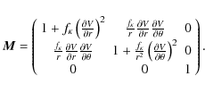
According to the standard theory of partial differential equations (PDEs) (e.g. Courant & Hilbert 1968, pp. 135), the class of a second order PDE is determined by the signs of the coefficients of the second derivatives after applying a local coordinate transformation (i.e. at fixed position) which leads to the coefficients of the mixed derivatives being zero.
Using the fundamental equation in the form (10) and rewriting it as
| (A.1) |
one can immediately see that only the first term matters for classification, because the second term contains only first derivatives. It is clear that the required transformation amounts to diagonalizing the matrix
|
|
(A.2) |
The matrix
Obviously, one eigenvalue is
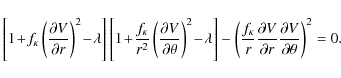
|
(A.4) |
The solutions of this quadratic equation are
References
- Al-Salti, N., Neukirch, T., & Ryan, R. 2010, A&A, 514, A38 [NASA ADS] [CrossRef] [EDP Sciences] [Google Scholar]
- Aulanier, G., Démoulin, P., Mein, N., et al. 1999, A&A, 342, 867 [NASA ADS] [Google Scholar]
- Bogdan, T. J., & Low, B. C. 1986, ApJ, 306, 271 [NASA ADS] [CrossRef] [Google Scholar]
- Courant, R., & Hilbert, D. 1968, Methoden der mathematischen Physik II (Berlin: Springer-Verlag) [Google Scholar]
- Donati, J.-F., Howarth, I. D., Jardine, M. M., et al. 2006, MNRAS, 370, 629 [NASA ADS] [CrossRef] [Google Scholar]
- Donati, J.-F., Morin, J., Petit, P., et al. 2008, MNRAS, 390, 545 [NASA ADS] [CrossRef] [Google Scholar]
- Gibson, S. E., & Bagenal, F. 1995, J. Geophys. Res., 100, 19865 [NASA ADS] [CrossRef] [Google Scholar]
- Gibson, S. E., Bagenal, F., & Low, B. C. 1996, J. Geophys. Res., 101, 4813 [NASA ADS] [CrossRef] [Google Scholar]
- Heinemann, M., & Olbert, S. 1978, J. Geophys. Res., 83, 2457 [NASA ADS] [CrossRef] [Google Scholar]
- Hussain, G. A. J., van Ballegooijen, A. A., Jardine, M., & Collier Cameron, A. 2002, ApJ, 575, 1078 [NASA ADS] [CrossRef] [Google Scholar]
- Jardine, M. 2004, A&A, 414, L5 [NASA ADS] [CrossRef] [EDP Sciences] [Google Scholar]
- Jardine, M., & Unruh, Y. C. 1999, A&A, 346, 883 [NASA ADS] [Google Scholar]
- Jardine, M., & van Ballegooijen, A. A. 2005, MNRAS, 361, 1173 [NASA ADS] [CrossRef] [Google Scholar]
- Jardine, M., Barnes, J. R., Donati, J.-F., & Collier Cameron, A. 1999, MNRAS, 305, L35 [NASA ADS] [CrossRef] [Google Scholar]
- Jardine, M., Collier Cameron, A., & Donati, J.-F. 2002, MNRAS, 333, 339 [NASA ADS] [CrossRef] [Google Scholar]
- Jardine, M., Collier Cameron, A., Donati, J.-F., & Pointer, G. R. 2001, MNRAS, 324, 201 [NASA ADS] [CrossRef] [Google Scholar]
- Kaiser, R., & Salat, A. 1996, , 77, 3133 [Google Scholar]
- Kaiser, R., & Salat, A. 1997, J. Plasma Phys., 57, 425 [NASA ADS] [CrossRef] [Google Scholar]
- Kaiser, R., Salat, A., & Tataronis, J. A. 1995, Phys. Plasmas, 2, 1599 [NASA ADS] [CrossRef] [Google Scholar]
- Lanza, A. F. 2008, A&A, 487, 1163 [NASA ADS] [CrossRef] [EDP Sciences] [Google Scholar]
- Lanza, A. F. 2009, A&A, 505, 339 [NASA ADS] [CrossRef] [EDP Sciences] [Google Scholar]
- Low, B. C. 1985, ApJ, 293, 31 [NASA ADS] [CrossRef] [Google Scholar]
- Low, B. C. 1991, ApJ, 370, 427 [NASA ADS] [CrossRef] [Google Scholar]
- Low, B. C. 1992, ApJ, 399, 300 [NASA ADS] [CrossRef] [Google Scholar]
- Low, B. C. 1993a, ApJ, 408, 689 [NASA ADS] [CrossRef] [Google Scholar]
- Low, B. C. 1993b, ApJ, 408, 693 [NASA ADS] [CrossRef] [Google Scholar]
- Low, B. C. 2005, ApJ, 625, 451 [NASA ADS] [CrossRef] [Google Scholar]
- Mestel, L. 1999, Stellar Magnetism (Oxford: Clarendon Press) [Google Scholar]
- Morin, J., Donati, J.-F., Petit, P., et al. 2008, MNRAS, 390, 567 [NASA ADS] [CrossRef] [MathSciNet] [Google Scholar]
- Neukirch, T. 1995, A&A, 301, 628 [NASA ADS] [Google Scholar]
- Neukirch, T. 1997, A&A, 325, 847 [NASA ADS] [Google Scholar]
- Neukirch, T. 2009, Geophys. Astrophys. Fluid Dyn., 103, 535 [NASA ADS] [CrossRef] [Google Scholar]
- Neukirch, T., & Rastätter, L. 1999, A&A, 348, 1000 [NASA ADS] [Google Scholar]
- Petrie, G. J. D., & Neukirch, T. 1999, Geophys. Astrophys. Fluid Dyn., 91, 269 [Google Scholar]
- Petrie, G. J. D., & Neukirch, T. 2000, A&A, 356, 735 [NASA ADS] [Google Scholar]
- Ruan, P., Wiegelmann, T., Inhester, B., et al. 2008, A&A, 481, 827 [NASA ADS] [CrossRef] [EDP Sciences] [Google Scholar]
- Rudenko, G. V. 2001, Sol. Phys., 198, 279 [NASA ADS] [CrossRef] [Google Scholar]
- Ryan, R. D., Neukirch, T., & Jardine, M. 2005, A&A, 433, 323 [NASA ADS] [CrossRef] [EDP Sciences] [Google Scholar]
- Salat, A., & Kaiser, R. 1995, Phys. Plasmas, 2, 3777 [NASA ADS] [CrossRef] [Google Scholar]
- Shivamoggi, B. K. 1986, Q. Appl. Math., 44, 487 [Google Scholar]
- Townsend, R. H. D., & Owocki, S. P. 2005, MNRAS, 357, 251 [NASA ADS] [CrossRef] [MathSciNet] [Google Scholar]
- Townsend, R. H. D., Owocki, S. P., & Groote, D. 2005, ApJ, 630, L81 [NASA ADS] [CrossRef] [Google Scholar]
- ud-Doula, A., Townsend, R. H. D., & Owocki, S. P. 2006, ApJ, 640, L191 [NASA ADS] [CrossRef] [Google Scholar]
- Wiegelmann, T., & Neukirch, T. 2006, A&A, 457, 1053 [NASA ADS] [CrossRef] [EDP Sciences] [Google Scholar]
- Wiegelmann, T., Neukirch, T., Ruan, P., & Inhester, B. 2007, A&A, 475, 701 [NASA ADS] [CrossRef] [EDP Sciences] [Google Scholar]
- Woolley, M. L. 1976, J. Plasma Phys., 15, 423 [NASA ADS] [CrossRef] [Google Scholar]
- Woolley, M. L. 1977, J. Plasma Phys., 17, 259 [NASA ADS] [CrossRef] [Google Scholar]
- Zhao, X., & Hoeksema, J. T. 1993, Sol. Phys., 143, 41 [NASA ADS] [CrossRef] [Google Scholar]
- Zhao, X., & Hoeksema, J. T. 1994, Sol. Phys., 151, 91 [Google Scholar]
- Zhao, X. P., Hoeksema, J. T., & Scherrer, P. H. 2000, ApJ, 538, 932 [NASA ADS] [CrossRef] [Google Scholar]
All Figures
|
|
Figure 1: Magnetic field line plots plots for the three cases of aligned rotator a), oblique rotator b) and displaced dipole c). The colours on the spherical surface represent the radial magnetic field component, Br on that boundary. |
| Open with DEXTER | |
| In the text | |
|
|
Figure 2:
Variation of the pressure deviation from the background pressure in the xz-plane at |
| Open with DEXTER | |
| In the text | |
|
|
Figure 3:
Variation of the density deviation from the background density in the xz-plane at |
| Open with DEXTER | |
| In the text | |
Copyright ESO 2010
Current usage metrics show cumulative count of Article Views (full-text article views including HTML views, PDF and ePub downloads, according to the available data) and Abstracts Views on Vision4Press platform.
Data correspond to usage on the plateform after 2015. The current usage metrics is available 48-96 hours after online publication and is updated daily on week days.
Initial download of the metrics may take a while.