| Issue |
A&A
Volume 520, September-October 2010
|
|
|---|---|---|
| Article Number | A53 | |
| Number of page(s) | 13 | |
| Section | Planets and planetary systems | |
| DOI | https://doi.org/10.1051/0004-6361/201014403 | |
| Published online | 04 October 2010 | |
Photospheric activity, rotation, and radial velocity variations of the planet-hosting star CoRoT-7![[*]](/icons/foot_motif.png)
A. F. Lanza1 - A. S. Bonomo1,2 - C. Moutou2 - I. Pagano1 - S. Messina1 - G. Leto1 - G. Cutispoto1 - S. Aigrain3 - R. Alonso4 - P. Barge2 - M. Deleuil2 - M. Auvergne5 - A. Baglin5 - A. Collier Cameron6
1 - INAF - Osservatorio Astrofisico di Catania, via S. Sofia 78, 95123 Catania, Italy
2 -
Laboratoire d'Astrophysique de Marseille (UMR 6110), Technopole de Château-Gombert,
38 rue Frédéric Joliot-Curie, 13388 Marseille Cedex 13, France
3 - Department of Physics, University of Oxford, Denys Wilkinson Building, Keble Road, Oxford OX1 3RH, UK
4 -
Observatoire de Genève, Université de Genève, 51 Ch. des Maillettes, 1290 Sauverny, Switzerland
5 -
LESIA, CNRS UMR 8109, Observatoire de Paris, 5 place J. Janssen, 92195 Meudon, France
6 -
School of Physics and Astronomy, University of St. Andrews, North Haugh, St Andrews, Fife KY16 9SS, Scotland
Received 11 March 2010 / Accepted 17 May 2010
Abstract
Context. The CoRoT satellite has recently discovered the
transits of an Earth-like planet across the disc of a late-type
magnetically active star dubbed CoRoT-7, while a second planet was
detected after filtering out the radial velocity (hereafter RV)
variations due to stellar activity.
Aims. We investigate the magnetic activity of CoRoT-7 and use
the results for a better understanding of the impact of magnetic
activity on stellar RV variations.
Methods. We derived the longitudinal distribution of active
regions on CoRoT-7 from a maximum entropy spot model of the CoRoT
lightcurve. Assuming that each active region consists of dark spots and
bright faculae in a fixed proportion, we synthesized the expected RV
variations.
Results. Active regions are mainly located at three active
longitudes that appear to migrate at different rates, probably as a
consequence of surface differential rotation, for which a lower limit
of
![]()
![]() 0.017 is found. The synthesized activity-induced RV variations
reproduce the amplitude of the observed RV curve and are used to study
the impact of stellar activity on planetary detection.
0.017 is found. The synthesized activity-induced RV variations
reproduce the amplitude of the observed RV curve and are used to study
the impact of stellar activity on planetary detection.
Conclusions. In spite of the non-simultaneous CoRoT and HARPS
observations, our study confirms the validity of the method previously
adopted to filter out RV variations induced by stellar activity.
We find a false-alarm probability
<10 -4 that the RV
oscillations attributed to CoRoT-7b and CoRoT-7c are spurious effects
of noise and activity. Additionally, our model suggests that other
periodicities found in the observed RV curve of CoRoT-7 could be
explained by active regions whose visibility is modulated by a
differential stellar rotation with periods ranging from 23.6 to
27.6 days.
Key words: stars: activity - stars: magnetic field - stars: late-type - stars: rotation - planetary systems - stars: individual: CoRoT-7
1 Introduction
CoRoT (Convection, Rotation and Transits) is a photometric space
experiment devoted to asteroseismology and the search for extrasolar
planets by the method of transits (Baglin et al. 2006).
It has recently discovered two Earth-like planets around a
late-type star called CoRoT-7, the innermost of which
transits across the disc of the star and has an orbital period of only
0.8536 days, while the other has a period of 3.69 days and
does not show transits (Queloz et al. 2009; Léger et al. 2009). The mass of the inner planet CoRoT-7b is 4.8 ![]()
![]() ,
while that of CoRoT-7c is 8.4
,
while that of CoRoT-7c is 8.4 ![]()
![]() ,
assuming they are on coplanar orbits (Queloz et al. 2009). The relative depth of the transit of CoRoT-7b is
,
assuming they are on coplanar orbits (Queloz et al. 2009). The relative depth of the transit of CoRoT-7b is
![]()
![]() 10-4 in the CoRoT white passband (see Sect. 2), leading to a planetary radius of 1.68
10-4 in the CoRoT white passband (see Sect. 2), leading to a planetary radius of 1.68 ![]()
![]() .
.
CoRoT-7 is an active star showing a rotational modulation of its optical flux with an amplitude up to
![]() mag and a period of
mag and a period of
![]() days (Queloz et al. 2009).
The discovery of CoRoT-7c and the measurement of the mass of CoRoT-7b
have become possible with the HARPS spectrograph after filtering out
the apparent variations of the stellar RV induced by magnetic activity
which have an amplitude of
days (Queloz et al. 2009).
The discovery of CoRoT-7c and the measurement of the mass of CoRoT-7b
have become possible with the HARPS spectrograph after filtering out
the apparent variations of the stellar RV induced by magnetic activity
which have an amplitude of
![]() m s-1,
i.e., 5-6 times greater than the wobbles produced by the
gravitational pull of the planets. Therefore, a more detailed
model of the stellar activity is needed to improve RV measurements
and to obtain better planetary parameters. This would also rule out the
possibility that a quasi-periodic RV signal is caused by rotating
spots on the stellar surface instead of a planetary companion as,
e.g., in the case of HD 166435 (Queloz et al. 2001).
m s-1,
i.e., 5-6 times greater than the wobbles produced by the
gravitational pull of the planets. Therefore, a more detailed
model of the stellar activity is needed to improve RV measurements
and to obtain better planetary parameters. This would also rule out the
possibility that a quasi-periodic RV signal is caused by rotating
spots on the stellar surface instead of a planetary companion as,
e.g., in the case of HD 166435 (Queloz et al. 2001).
We applied the same spot modelling approach as used for the high-precision lightcurves of CoRoT-2 (Lanza et al. 2009a) and CoRoT-4 (Lanza et al. 2009b) to derive the longitudinal distribution of photospheric brightness inhomogeneities and their evolution during the ![]() days
of CoRoT observations. The different rotation rates of active regions
allowed us to estimate a lower limit for the amplitude of the
differential rotation of CoRoT-7. From our spot maps, we synthesized
the activity-induced RV perturbations using a simple model for the
distortion of the line profiles, as described in Sect. 3.2.
A Fourier analysis of such a synthetic time series yielded typical
periods induced by stellar activity, allowing us to discuss its impact
on the detection of planets around CoRoT-7.
days
of CoRoT observations. The different rotation rates of active regions
allowed us to estimate a lower limit for the amplitude of the
differential rotation of CoRoT-7. From our spot maps, we synthesized
the activity-induced RV perturbations using a simple model for the
distortion of the line profiles, as described in Sect. 3.2.
A Fourier analysis of such a synthetic time series yielded typical
periods induced by stellar activity, allowing us to discuss its impact
on the detection of planets around CoRoT-7.
2 Observations
CoRoT-7 was observed during the first long run of CoRoT toward the
galactic anticentre from 24 October 2007 to
3 March 2008. Since the star is bright (V
=11.67), the time sampling is 32 s from the beginning of the
observations. CoRoT performs aperture photometry with a fixed mask (see
Fig. 6 in Léger et al. 2009).
The contaminating flux from background stars falling inside the mask
amounts to a maximum of 0.9 percent and produces a dilution of the
photometric variation of CoRoT-7 lower than 1.8 ![]() 10-4 mag that can be safely ignored for our purposes (see Léger et al. 2009,
for upper limits on the background flux variations). The flux inside
the star's mask is split along detector column boundaries into
broad-band red, green, and blue channels.
10-4 mag that can be safely ignored for our purposes (see Léger et al. 2009,
for upper limits on the background flux variations). The flux inside
the star's mask is split along detector column boundaries into
broad-band red, green, and blue channels.
The observations and data processing are described by Léger et al. (2009), to whom we refer the reader for details. The reduction pipeline applies corrections for the sky background and the pointing jitter of the satellite, which is particularly relevant during ingress and egress from the Earth shadow. Measurements during the crossing of the South Atlantic Anomaly of the Earth's magnetic field, which amounts to about 7-9 percent of each satellite orbit, are discarded. High-frequency spikes due to cosmic ray hits and outliers are removed by applying a 7-point running mean. The final duty cycle of the 32-s observations is 88.8 percent for the so-called N2 data time series that are accessible through the CoRoT Public Data Archive at the IAS (http://idoc-corot.ias.u-psud.fr/). To increase the signal-to-noise ratio and reduce systematic drifts present in individual channels, we summed up the flux in the red, green, and blue channels to obtain a lightcurve in a spectral range extending from 300 to 1100 nm. More information on the instrument, its operation, and performance can be found in Auvergne et al. (2009).
The transits are removed using the ephemeris of Léger et al. (2009)
and the out-of-transit data are binned by computing average flux values
along each orbital period of the satellite (6184 s). This has the
advantage of removing tiny systematic variations associated with the
orbital motion of the satellite (cf. Auvergne et al. 2009; Alonso et al. 2008).
In such a way we obtain a lightcurve consisting of
1793 average points ranging from HJD 2 454 398.0719
to HJD 2 454 528.8877, i.e., with a duration of
130.8152 days. The average standard deviation of the points is
2.678 ![]() 10-4
in relative flux units. The maximum observed flux in the average point
time series at HJD 2 454 428.4232 is adopted as a
reference unit level corresponding to the unspotted star, since the
true value of the unspotted flux is unknown.
10-4
in relative flux units. The maximum observed flux in the average point
time series at HJD 2 454 428.4232 is adopted as a
reference unit level corresponding to the unspotted star, since the
true value of the unspotted flux is unknown.
3 Lightcurve and radial velocity modelling
3.1 Spot modelling of wide-band lightcurves
The reconstruction of the surface brightness distribution from the
rotational modulation of the stellar flux is an ill-posed problem,
because the variation in the flux vs. rotational phase only
contains information on the distribution of the brightness
inhomogeneities vs. longitude. The integration over the stellar
disc effectively cancels any latitudinal information, particularly when
the inclination of the rotation axis along the line of sight is close
to
![]() ,
as assumed in the present case (see Sect. 4 and Lanza et al. 2009a).
Therefore, we need to include a priori information in the
lightcurve inversion process to obtain a unique and stable map. This is
done by computing a maximum entropy (hereafter ME) map, which has
been proven to successfully reproduce active region distribution and
area variations in the case of the Sun (cf. Lanza et al. 2007).
,
as assumed in the present case (see Sect. 4 and Lanza et al. 2009a).
Therefore, we need to include a priori information in the
lightcurve inversion process to obtain a unique and stable map. This is
done by computing a maximum entropy (hereafter ME) map, which has
been proven to successfully reproduce active region distribution and
area variations in the case of the Sun (cf. Lanza et al. 2007).
In our model, the star is subdivided into 200 surface elements, namely 200 squares with sides of
![]() ,
with each element containing unperturbed photosphere, dark spots, and
facular areas. The fraction of an element covered by dark spots is
indicated by the filling factor f, the fractional area of the faculae is Qf, and the fractional area of the unperturbed photosphere is 1-(Q+1)f. The contribution to the stellar flux coming from the kth surface element at the time tj, where
j=1,..., N, is an index numbering the N points along the lightcurve, is given by
,
with each element containing unperturbed photosphere, dark spots, and
facular areas. The fraction of an element covered by dark spots is
indicated by the filling factor f, the fractional area of the faculae is Qf, and the fractional area of the unperturbed photosphere is 1-(Q+1)f. The contribution to the stellar flux coming from the kth surface element at the time tj, where
j=1,..., N, is an index numbering the N points along the lightcurve, is given by
where I0 is the specific intensity in the continuum of the unperturbed photosphere at the isophotal wavelength of the observations,
|
(2) |
is its visibility, and
![\begin{displaymath}%
\mu_{kj} \equiv \cos \psi_{kj} = \sin i \sin \theta_{k} \cos [\ell_{k} + \Omega (t_{j}-t_{0})] + \cos i \cos \theta_{k}
\end{displaymath}](/articles/aa/full_html/2010/12/aa14403-10/img29.png)
is the cosine of the angle
We fit the lightcurve by varying the value of f over the surface of the star, while Q is held constant. Even after we fix the rotation period, the inclination, and the spot and facular contrasts (see Lanza et al. 2007,
for details), the model has 200 free parameters and suffers from
non-uniqueness and instability. To find a unique and stable spot map,
we apply ME regularization, as described in Lanza et al. (2007), by minimizing a functional Z, which is a linear combination of the ![]() and the entropy functional S; i.e.,
and the entropy functional S; i.e.,
|
(4) |
where
In the case of the Sun, by assuming a fixed distribution of the filling
factor, it is possible to obtain a good fit of the irradiance
changes only for a limited time interval
![]() ,
not exceeding 14 days, which is the lifetime of the largest
sunspot groups dominating the irradiance variation. For other active
stars, the value of
,
not exceeding 14 days, which is the lifetime of the largest
sunspot groups dominating the irradiance variation. For other active
stars, the value of
![]() must
be determined from the observations themselves, looking for the longest
time interval that allows a good fit with the applied model
(see Sect. 4).
must
be determined from the observations themselves, looking for the longest
time interval that allows a good fit with the applied model
(see Sect. 4).
The optimal values of the spot and facular contrasts and of the facular-to-spotted area ratio Q in stellar active regions are unknown a priori. In our model the facular contrast ![]() and the parameter Q enter as the product
and the parameter Q enter as the product
![]() ,
so we can fix
,
so we can fix ![]() and vary Q, estimating its best value by minimizing the
and vary Q, estimating its best value by minimizing the ![]() of the model, as shown in Sect. 4. Since there are many free parameters in the ME model, for this specific application we make use of the model of Lanza et al. (2003),
which fits the lightcurve by assuming only three active regions to
model the rotational modulation of the flux plus a uniformly
distributed background to account for the variations in the mean light
level. This procedure is the same as was used to fix the value of Q in the cases of CoRoT-2 and CoRoT-4 (cf. Lanza et al. 2009a,b).
of the model, as shown in Sect. 4. Since there are many free parameters in the ME model, for this specific application we make use of the model of Lanza et al. (2003),
which fits the lightcurve by assuming only three active regions to
model the rotational modulation of the flux plus a uniformly
distributed background to account for the variations in the mean light
level. This procedure is the same as was used to fix the value of Q in the cases of CoRoT-2 and CoRoT-4 (cf. Lanza et al. 2009a,b).
We assume an inclination of the rotation axis of CoRoT-7 of
![]() (see Sect. 4).
Since the information on spot latitude that can be extracted from the
rotational modulation of the flux for such a high inclination is
negligible, the ME regularization virtually puts all the spots at
the sub-observer latitude (i.e.,
(see Sect. 4).
Since the information on spot latitude that can be extracted from the
rotational modulation of the flux for such a high inclination is
negligible, the ME regularization virtually puts all the spots at
the sub-observer latitude (i.e.,
![]() )
to minimize their area and maximize the entropy. Therefore, we are
limited to mapping only the distribution of the active regions vs.
longitude, which can be done with a resolution higher than
)
to minimize their area and maximize the entropy. Therefore, we are
limited to mapping only the distribution of the active regions vs.
longitude, which can be done with a resolution higher than
![]() (cf. Lanza et al. 2009a,2007).
Our ignorance of the true facular contribution may lead to systematic
errors in the active region longitudes derived by our model because
faculae produce an increase in the flux when they are close to the
limb, leading to a systematic shift in the longitudes of the active
regions used to reproduce the observed flux modulation,
as discussed by Lanza et al. (2007) for the Sun and illustrated by Lanza et al. (2009a, cf. Figs. 4 and 5# for CoRoT-2.
(cf. Lanza et al. 2009a,2007).
Our ignorance of the true facular contribution may lead to systematic
errors in the active region longitudes derived by our model because
faculae produce an increase in the flux when they are close to the
limb, leading to a systematic shift in the longitudes of the active
regions used to reproduce the observed flux modulation,
as discussed by Lanza et al. (2007) for the Sun and illustrated by Lanza et al. (2009a, cf. Figs. 4 and 5# for CoRoT-2.
3.2 Activity-induced radial velocity variations
Surface magnetic fields in late-type stars produce brightness and
convection inhomogeneities that shift and distort their spectral line
profiles leading to apparent RV variations (cf., e.g., Huber et al. 2009; Saar & Donahue 1997; Saar et al. 1998).
To compute the apparent RV variations induced by stellar active
regions, we adopt a simple model for each line profile considering the
residual profile
![]() at a wavelength
at a wavelength ![]() along the line, i.e.:
along the line, i.e.:
![]() ,
where
,
where
![]() is the specific intensity at wavelength
is the specific intensity at wavelength ![]() and
and ![]() the
intensity in the continuum adjacent to the line. The local residual
profile is assumed to have a Gaussian shape with thermal and
microturbulent width
the
intensity in the continuum adjacent to the line. The local residual
profile is assumed to have a Gaussian shape with thermal and
microturbulent width
![]() (cf., e.g., Gray 1988, Ch. 1); i.e.,
(cf., e.g., Gray 1988, Ch. 1); i.e.,
![\begin{displaymath}%
R(\lambda) \propto \exp \left[- \left( \frac{\lambda -\lambda_{0}}{\Delta \lambda_{\rm D}} \right)^{2} \right],
\end{displaymath}](/articles/aa/full_html/2010/12/aa14403-10/img62.png)
where
To include the effects of surface magnetic fields on convective
motions, we consider the decrease of macroturbulence velocity and the
reduction of convective blueshifts in active regions. Specifically, we
assume a local radial-tangential macroturbulence, as introduced by
Gray (1988), with a distribution function ![]() for the radial velocity v of the form:
for the radial velocity v of the form:
![\begin{displaymath}%
\Theta (v, \mu) = \frac{1}{2} \frac{\exp \left[- \left( \fr...
... RT} \mu} \right)^{2} \right]}{\sqrt{\pi} \zeta_{\rm RT} \mu},
\end{displaymath}](/articles/aa/full_html/2010/12/aa14403-10/img65.png)
where
Convective blueshifts arise from the fact that in stellar photospheres
most of the flux comes from the extended updrafts at the centre of
convective granules. At the centre of the stellar disc, the
vertical component of the convective velocity produces a maximum
blueshift, while the effect vanishes at the limb where the projected
velocity is zero. The cores of the deepest spectral lines form in the
upper layers of the photosphere where the vertical convective velocity
is low, while the cores of shallow lines form in deeper layers with
higher vertical velocity. Therefore, the cores of shallow lines are
blueshifted with respect to the cores of the deepest lines. Gray (2009)
shows this effect by plotting the endpoints of line bisectors of
shallow and deep lines on the same velocity scale. He shows that
the amplitude of the relative blueshifts scales with the spectral type
and the luminosity class of the star. For the G8V star ![]() Ceti,
which has a spectral type close to the G9V of CoRoT-7, the convective
blueshifts should be similar to those of the Sun, so we adopt solar
values in our simulations. In active regions, vertical convective
motions are quenched, so we observe an apparent redshift of the
spectral lines in spotted and facular areas in comparison to the
unperturbed photosphere. Meunier et al. (2010) quantify this effect in the case of the Sun, and we adopt their results, considering an apparent redshift
Ceti,
which has a spectral type close to the G9V of CoRoT-7, the convective
blueshifts should be similar to those of the Sun, so we adopt solar
values in our simulations. In active regions, vertical convective
motions are quenched, so we observe an apparent redshift of the
spectral lines in spotted and facular areas in comparison to the
unperturbed photosphere. Meunier et al. (2010) quantify this effect in the case of the Sun, and we adopt their results, considering an apparent redshift
![]() m s-1 in faculae and
m s-1 in faculae and
![]() m s-1 in cool spots.
m s-1 in cool spots.
In principle, the integrated effect of convective redshifts can be measured in a star by comparing RV measurements obtained with two different line masks, one including the shallow lines and the other the deep lines (cf. Meunier et al. 2010). For CoRoT-7, which lacks such measurements, we apply the results of Gray (2009) and adopt solar-like values as the best approximation.
Considering solar convection as a template, intense downdrafts are localized in the dark lanes at the boundaries of the upwelling granules, but they contribute a significantly smaller flux because of their lower brightness and smaller area. While a consideration of those downdrafts is needed to simulate the shapes of line bisectors, it is beyond the scope of our simplified approach that assumes that the whole profile of our template line forms at the same depth inside the photosphere. Therefore, we restrict our model to the mean apparent RV variations by neglecting the associated variations of the bisector shape and do not include the effect of convective downdrafts, as well as those of other surface flows typical of solar active regions, such as the Evershed effect in sunspots (cf., e.g., Meunier et al. 2010).
The local central wavelength
![]() of the kth surface element at time tj is given by
of the kth surface element at time tj is given by
![]() ,
where vkj is its radial velocity,
,
where vkj is its radial velocity,
![\begin{displaymath}%
v_{kj} = - (v \sin i) \sin \theta_{k} \sin [\ell_{k} + \Omega (t_{j} - t_{0})] + \Delta V_{\rm cs},
\end{displaymath}](/articles/aa/full_html/2010/12/aa14403-10/img74.png)
|
(7) |
with c the speed of light,
|
(8) |
where fk is the spot filling factor of the element, Q the facular-to-spotted area ratio, and
We integrate the line specific intensity at a given wavelength over the disc of the star using a subdivision into ![]()
![]()
![]() surface elements to obtain the flux along the line profile
surface elements to obtain the flux along the line profile
![]() at a given time tj. To find the apparent stellar RV, we can fit a Gaussian to the line profile
at a given time tj. To find the apparent stellar RV, we can fit a Gaussian to the line profile
![]() ,
or we can determine the centroid of the profile as
,
or we can determine the centroid of the profile as
where
A single line profile computed with the above model can be regarded as a cross-correlation function (hereafter CCF) obtained by cross-correlating the whole stellar spectrum with a line mask consisting of Dirac delta functions giving the rest wavelength and depth of each individual line (e.g., Queloz et al. 2001). Therefore, to derive the RV from a single synthetic line profile is equivalent to measuring the RV from a CCF, either by fitting it with a Gaussian or by computing its centroid wavelength. A better approach would be to simulate the whole stellar optical spectrum or an extended section of it to account for the wavelength dependence of the spot and facular contrasts, as well as of the convective inhomogeneities (cf., e.g., Meunier et al. 2010; Lagrange et al. 2010; Desort et al. 2007). Again, in view of our limited knowledge of the distribution of active regions on the stellar surface, our simplified approach is adequate for estimating the RV perturbations induced by magnetic fields.
3.2.1 Some illustrative examples
To illustrate how active regions affect the measurement of stellar RV,
we consider the simple case of a single active region on a slowly
rotating star, assuming stellar parameters similar to the cases
presented by Saar & Donahue (1997) and Desort et al. (2007) for comparison purposes. Specifically, we adopt
![]() km s-1 and a macroturbulence
km s-1 and a macroturbulence
![]() km s-1
to make macroturbulence effects visible. For the moment, we do not
include convective redshifts in spots and faculae because they were not
taken into account in those simulations. We consider a single active
region of square shape
km s-1
to make macroturbulence effects visible. For the moment, we do not
include convective redshifts in spots and faculae because they were not
taken into account in those simulations. We consider a single active
region of square shape
![]()
![]()
![]() located at the equator of a star observed equator-on, to maximize the
RV variation. The spot filling factor is assumed to be f=0.99 and their contrast
located at the equator of a star observed equator-on, to maximize the
RV variation. The spot filling factor is assumed to be f=0.99 and their contrast
![]() ,
i.e., the spot effective temperature is much lower than the photospheric temperature. When faculae are included, we adopt
,
i.e., the spot effective temperature is much lower than the photospheric temperature. When faculae are included, we adopt
![]() and Q=9 to make their contribution clearly evident. In Fig. 1
we show the apparent RV and the relative flux variations produced by
the active region vs. the rotation phase. The RV variations
are computed by fitting a Gaussian to the line profile, as in Saar & Donahue (1997),
while by applying the centroid method we find values that differ by at
most 10-15 percent. The greatest apparent variation is obtained in
the case of a purely dark spot without any bright facula or reduced
macroturbulence. In this case, the line profile integrated over
the stellar disc shows a bump at the RV of the spot because the
intensity of the local continuum is reduced in the spot (see Fig. 1 in Vogt & Penrod 1983, for an illustration of the effect). A comparison with the amplitudes calculated with the formulae of Saar & Donahue (1997) or Desort et al. (2007) shows agreement within
and Q=9 to make their contribution clearly evident. In Fig. 1
we show the apparent RV and the relative flux variations produced by
the active region vs. the rotation phase. The RV variations
are computed by fitting a Gaussian to the line profile, as in Saar & Donahue (1997),
while by applying the centroid method we find values that differ by at
most 10-15 percent. The greatest apparent variation is obtained in
the case of a purely dark spot without any bright facula or reduced
macroturbulence. In this case, the line profile integrated over
the stellar disc shows a bump at the RV of the spot because the
intensity of the local continuum is reduced in the spot (see Fig. 1 in Vogt & Penrod 1983, for an illustration of the effect). A comparison with the amplitudes calculated with the formulae of Saar & Donahue (1997) or Desort et al. (2007) shows agreement within ![]() percent.
The RV perturbation is positive and the flux decreases when the spot is
on the approaching half of the disc. When the spot transits across the
central meridian, the RV perturbation becomes zero and the flux
reaches a relative minimum. Finally, the RV perturbation becomes
negative when the spot is on the receding half of the disc and the flux
is increasing.
percent.
The RV perturbation is positive and the flux decreases when the spot is
on the approaching half of the disc. When the spot transits across the
central meridian, the RV perturbation becomes zero and the flux
reaches a relative minimum. Finally, the RV perturbation becomes
negative when the spot is on the receding half of the disc and the flux
is increasing.
![\begin{figure}
\par\includegraphics[height=10cm,width=6.6cm,clip]{14403f1.ps}
\end{figure}](/articles/aa/full_html/2010/12/aa14403-10/img89.png)
|
Figure 1: Apparent RV variation (upper panel) and relative stellar flux (lower panel) vs. the rotation phase produced by a single active region on a star seen equator-on. Different linestyles indicate different kinds of inhomogeneities inside the active region. Dashed: reduced macroturbulence without brightness perturbation; solid: dark spot and reduced macroturbulence; dotted: dark spot, bright facula, and reduced macroturbulence. The flux is measured in units of the unperturbed stellar flux. |
| Open with DEXTER | |
Including the radial-tangential macroturbulence produces a decrease in the RV amplitude because macroturbulence is reduced in spots so that the local line profile becomes narrower and deeper, while its equivalent width is not significantly affected (Gray 1988). This reduces the height of the bump in the integrated profile acting in the opposite direction to the perturbation produced by a dark spot, as is evident in the case where only a macroturbulence reduction is included in the model. The wide-band flux variations are not affected by including the macroturbulence in any case.
The effect of the faculae is to increase the local continuum intensity
when an active region is close to the limb, leading to more local
absorption, which produces a dip in the integrated line profile. Since
the contrast of the faculae is greatly reduced when they move close to
the centre of the disc, this has the effect of narrowing the
RV peak produced by an active region when dark spots and faculae
are simultaneously present, i.e., faculae increase the frequency
of the RV variation. Specifically, the frequency of the
RV variation in the case of a single active region is twice the
rotation frequency when dark spots or a reduction of the
macroturbulence are present (cf. Fig. 1,
upper panel, where we see a complete RV oscillation along one
transit of the active region that lasts half a stellar rotation).
Including solar-like faculae can increase the frequency of the
variation up to four times the rotation frequency when facular effects
gain in significance (i.e.,
![]() ). This is illustrated in the upper panel of Fig. 2
with the RV variation produced by an active region with a sizeable
facular contribution (see below) showing two complete oscillations
along one transit.
). This is illustrated in the upper panel of Fig. 2
with the RV variation produced by an active region with a sizeable
facular contribution (see below) showing two complete oscillations
along one transit.
Next we consider the apparent redshifts due to the reduction of
convective blueshifts in spots and faculae. To make the effect evident,
now we adopt a spot contrast
![]() ,
a facular contrast
,
a facular contrast
![]() ,
and Q = 4.5. For the convective redshifts, we assume
,
and Q = 4.5. For the convective redshifts, we assume
![]() m s-1 and
m s-1 and
![]() m s-1. A lower spot contrast, e.g.,
m s-1. A lower spot contrast, e.g.,
![]() ,
as in the previous simulations, makes the contribution of the
local redshifted line profile coming from the spotted area very small,
reducing the corresponding RV perturbation. In Fig. 2
(upper panel), we plot the RV variation produced by the single
active region previously considered, with all the other parameters kept
at the previous values. For the purpose of comparison, we also plot the
RV perturbation obtained without convective redshifts.
In this case, the effects of cool spots and bright faculae almost
balance each other out because of the higher spot contrast, and the
oscillation of the RV shows a high frequency. On the other hand,
including convective redshifts brings the frequency of the
RV variation close to the rotation frequency, with a single
maximum per rotation. This happens because the perturbation is always
positive, while all the other effects change their sign when the active
region transits from the approaching to the receding half of the
stellar disc. Moreover, the convective redshifts do not depend per se
on the contrast factors
,
as in the previous simulations, makes the contribution of the
local redshifted line profile coming from the spotted area very small,
reducing the corresponding RV perturbation. In Fig. 2
(upper panel), we plot the RV variation produced by the single
active region previously considered, with all the other parameters kept
at the previous values. For the purpose of comparison, we also plot the
RV perturbation obtained without convective redshifts.
In this case, the effects of cool spots and bright faculae almost
balance each other out because of the higher spot contrast, and the
oscillation of the RV shows a high frequency. On the other hand,
including convective redshifts brings the frequency of the
RV variation close to the rotation frequency, with a single
maximum per rotation. This happens because the perturbation is always
positive, while all the other effects change their sign when the active
region transits from the approaching to the receding half of the
stellar disc. Moreover, the convective redshifts do not depend per se
on the contrast factors ![]() and
and ![]() ,
and the shift due to the faculae is amplified by the facular-to-spotted area ratio Q.
The modulation of the continuum flux is of course not affected by the
convective shifts, so we obtain the same lightcurve independent of
the value of
,
and the shift due to the faculae is amplified by the facular-to-spotted area ratio Q.
The modulation of the continuum flux is of course not affected by the
convective shifts, so we obtain the same lightcurve independent of
the value of
![]() and
and
![]() (cf. Fig. 2, lower panel).
(cf. Fig. 2, lower panel).
Particularly for not too dark spots (i.e.,
![]() )
and small
)
and small ![]() ,
convective redshifts cannot be neglected, therefore, in the simulation
of the activity-induced RV perturbations in solar-like stars,
as pointed out by Meunier et al. (2010).
In the case of the Sun, redshifts not only increase the
RV perturbation up to an order of magnitude, but also bring its
dominant period close to the solar rotation period, while without
including them those authors find that the dominant period corresponds
to the first harmonic of the solar rotation period.
,
convective redshifts cannot be neglected, therefore, in the simulation
of the activity-induced RV perturbations in solar-like stars,
as pointed out by Meunier et al. (2010).
In the case of the Sun, redshifts not only increase the
RV perturbation up to an order of magnitude, but also bring its
dominant period close to the solar rotation period, while without
including them those authors find that the dominant period corresponds
to the first harmonic of the solar rotation period.
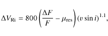
The amplitude of the RV variation produced by an active region depends
on several parameters that are poorly known, i.e., the latitude of
the active region, the spot and facular contrasts, the convective
redshifts, and the macroturbulence parameter that is difficult to
disentangle from rotational broadening in a slowly rotating star such
as CoRoT-7 (Léger et al. 2009). Moreover, the spot and facular contrasts depend on the wavelength (Lanza et al. 2004), leading to a difference of
![]() percent in the RV variations as derived from different orders of an echelle spectrum (cf., e.g., Desort et al. 2007), and the convective redshift depends on the formation depth of a spectral line.
percent in the RV variations as derived from different orders of an echelle spectrum (cf., e.g., Desort et al. 2007), and the convective redshift depends on the formation depth of a spectral line.
The simultaneous presence of several active regions gives rise to a complex line profile distortion for a slowly rotating star because the perturbations of different regions overlap in the line profile owing to the weak rotational broadening. This implies an additional 15-20 percent uncertainty in the determination of the shift of the profile by the Gaussian fit or the centroid method, as found by comparing the RV determinations obtained with the two methods in the case of line profiles simulated with infinite signal-to-noise ratio and perfectly regular sampling. In consideration of all these limitations, the absolute values of the RV variations computed with our model are uncertain by 20-30 percent for complex distributions of active regions, such as those derived by our spot modelling technique as applied to CoRoT-7 lightcurves.
![\begin{figure}
\par\includegraphics[height=7.8cm,width=6.6cm,clip]{14403f2.ps}
\vspace*{-3mm}
\end{figure}](/articles/aa/full_html/2010/12/aa14403-10/img98.png)
|
Figure 2: Same as Fig. 1 when including (solid line) and not including (dotted line) the convective redshifts in cool spots and bright faculae in the simulation (see the text for the active region parameters). |
| Open with DEXTER | |
3.2.2 Radial velocity variations from spot modelling
We can use the distribution of active regions as derived from our spot
modelling to synthesize the corresponding RV variations according
to the approach outlined in Sect. 3.2. Since our spot model assumes that active regions are stable for the time interval of each fitted time series
![]() ,
the distribution of surface inhomogeneities can be used to synthesize the RV variations having a timescale of
,
the distribution of surface inhomogeneities can be used to synthesize the RV variations having a timescale of
![]() or longer. Active regions with shorter lifetimes produce a photometric
modulation that appears in the residuals of the best fit to the
lightcurve. As we see in Sect. 5.1,
most of the short-term variability occurs on timescales of
4-5 days, i.e., significantly shorter than the rotation
period of CoRoT-7, so we can neglect, as a first approximation,
the variation in the disc position of active regions due to stellar
rotation and estimate their area as if they were located at the centre
of the disc.
Specifically, we first express the residuals as the relative
deviation
or longer. Active regions with shorter lifetimes produce a photometric
modulation that appears in the residuals of the best fit to the
lightcurve. As we see in Sect. 5.1,
most of the short-term variability occurs on timescales of
4-5 days, i.e., significantly shorter than the rotation
period of CoRoT-7, so we can neglect, as a first approximation,
the variation in the disc position of active regions due to stellar
rotation and estimate their area as if they were located at the centre
of the disc.
Specifically, we first express the residuals as the relative
deviation
![]() between the observed flux and its best fit measured in units of the reference unspotted flux F0. Then we subtract its mean value
between the observed flux and its best fit measured in units of the reference unspotted flux F0. Then we subtract its mean value
![]() from
from
![]() because
the mean value corresponds to a uniformly distributed population of
active regions that do not produce any RV variation. At each
given time t, we adopt the relative deviation
because
the mean value corresponds to a uniformly distributed population of
active regions that do not produce any RV variation. At each
given time t, we adopt the relative deviation
![]() as a measure of the filling factor of the active regions producing the
short-term RV variations. In doing so, we neglect
limb-darkening effects and assume that those active regions consist of
completely dark spots (
as a measure of the filling factor of the active regions producing the
short-term RV variations. In doing so, we neglect
limb-darkening effects and assume that those active regions consist of
completely dark spots (
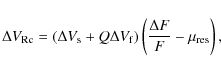
![]() ). Finally, we compute the RV perturbation due to such brightness inhomogeneities by means of Eq. (1) of Desort et al. (2007) obtaining
). Finally, we compute the RV perturbation due to such brightness inhomogeneities by means of Eq. (1) of Desort et al. (2007) obtaining
where the RV perturbation is measured in m s-1 and the
where the sign of
4 Model parameters
The fundamental stellar parameters are taken from Léger et al. (2009) and are listed in
Table 1. The limbdarkening parameters ![]() ,
,
![]() ,
and
,
and ![]() (cf. Sect. 3.1) have been derived from Kurucz (2000) model atmospheres for
(cf. Sect. 3.1) have been derived from Kurucz (2000) model atmospheres for
![]() K,
K,
![]() (cm s-2) and solar abundances, by adopting the CoRoT white-band transmission profile given by Auvergne et al. (2009). Recently, Bruntt et al. (2010)
have slightly revised stellar parameters, but adopting their values
does not produce any significant modification in our modelling.
(cm s-2) and solar abundances, by adopting the CoRoT white-band transmission profile given by Auvergne et al. (2009). Recently, Bruntt et al. (2010)
have slightly revised stellar parameters, but adopting their values
does not produce any significant modification in our modelling.
The rotation period adopted for our spot modelling has been derived from a periodogram analysis of the lightcurve giving
![]()
![]() 3.62 days.
The uncertainty of this period determination is derived from the total
extension of the time series and represents an upper limit.
As seen below, our spot model shows that the starspots have a
remarkable differential rotation which contributes to an uncertainty of
the stellar rotation period of
3.62 days.
The uncertainty of this period determination is derived from the total
extension of the time series and represents an upper limit.
As seen below, our spot model shows that the starspots have a
remarkable differential rotation which contributes to an uncertainty of
the stellar rotation period of ![]() percent, i.e., of
percent, i.e., of ![]() days (cf. Sect. 5.2).
days (cf. Sect. 5.2).
Table 1: Parameters adopted for the lightcurve and RV modelling of CoRoT-7.
The polar flattening of the star because of the centrifugal potential
is computed in the Roche approximation with a rotation period of
23.64 days. The relative difference between the equatorial and the
polar radii ![]() is 8.54
is 8.54 ![]() 10-6, which induces a completely negligible relative flux variation of
10-6, which induces a completely negligible relative flux variation of
![]() for a spot coverage of
for a spot coverage of ![]() percent as a consequence of the gravity darkening of the equatorial region of the star.
percent as a consequence of the gravity darkening of the equatorial region of the star.
The inclination of the stellar rotation axis is impossible to constrain
through the observation of the Rossiter-McLaughlin effect owing to the
very small planet relative radius
![]()
![]() 3.0
3.0 ![]() 10-4, the small rotational broadening of the star
10-4, the small rotational broadening of the star
![]() km s-1, and its intrinsic line profile variations due to stellar activity (Queloz et al. 2009).
Nevertheless, we assume that the stellar rotation axis is orthogonal to
the orbital plane of the transiting planet, i.e., with an
inclination of
km s-1, and its intrinsic line profile variations due to stellar activity (Queloz et al. 2009).
Nevertheless, we assume that the stellar rotation axis is orthogonal to
the orbital plane of the transiting planet, i.e., with an
inclination of
![]()
![]()
![]() from the line of sight (cf. Léger et al. 2009).
from the line of sight (cf. Léger et al. 2009).
The maximum time interval that our model can accurately fit with a fixed distribution of active regions
![]() was determined by dividing the total interval,
T= 130.8152 days, into
was determined by dividing the total interval,
T= 130.8152 days, into ![]() equal segments, i.e.,
equal segments, i.e.,
![]() ,
and looking for the minimum value of
,
and looking for the minimum value of ![]() that allows a good fit of the lightcurve, as measured by the
that allows a good fit of the lightcurve, as measured by the ![]() statistics. We found that for
statistics. We found that for
![]() the quality of the best fit degraded significantly with respect to
the quality of the best fit degraded significantly with respect to
![]() ,
owing to a substantial evolution of the pattern of surface brightness inhomogeneities. Therefore, we adopt
,
owing to a substantial evolution of the pattern of surface brightness inhomogeneities. Therefore, we adopt
![]() days
as the maximum time interval to be fitted with a fixed distribution of
surface active regions in order to estimate the best value of the
parameter Q (see below). This confirms the result of Queloz et al. (2009), who estimate a starspot coherence time of
days
as the maximum time interval to be fitted with a fixed distribution of
surface active regions in order to estimate the best value of the
parameter Q (see below). This confirms the result of Queloz et al. (2009), who estimate a starspot coherence time of ![]() days. However, for the spot modelling in Sects. 5.1 and 5.2, we adopt
days. However, for the spot modelling in Sects. 5.1 and 5.2, we adopt
![]() ,
corresponding to
,
corresponding to
![]() days,
which provides better time resolution for studying the evolution of the
spot pattern during the intervals with faster modifications.
days,
which provides better time resolution for studying the evolution of the
spot pattern during the intervals with faster modifications.
To compute the spot contrast, we adopt the same mean temperature
difference as derived for sunspot groups from their bolometric
contrast, i.e., 560 K (Chapman et al. 1994). In other words, we assume a spot effective temperature of 4715 K, yielding a contrast
![]() in the CoRoT passband (cf. Lanza et al. 2007).
A different spot contrast changes the absolute spot coverages, but
does not significantly affect their longitudes and their time
evolution, as discussed in detail by Lanza et al. (2009a). The facular contrast is assumed to be solar-like with
in the CoRoT passband (cf. Lanza et al. 2007).
A different spot contrast changes the absolute spot coverages, but
does not significantly affect their longitudes and their time
evolution, as discussed in detail by Lanza et al. (2009a). The facular contrast is assumed to be solar-like with
![]() (Lanza et al. 2004).
(Lanza et al. 2004).
The best value of the area ratio Q of the faculae to the spots in each active region was estimated by means of the model of Lanza et al. (2003, cf. Sect. 3.1). In Fig. 3, we plot the ratio
![]() of the total
of the total ![]() of the composite best fit of the entire time series to its minimum value
of the composite best fit of the entire time series to its minimum value
![]() ,
versus Q, and indicate the 95 percent confidence level as derived from the F-statistics (e.g., Lampton et al. 1976). After choosing
,
versus Q, and indicate the 95 percent confidence level as derived from the F-statistics (e.g., Lampton et al. 1976). After choosing
![]() days,
we fit the rotational modulation of the active regions for the longest
time interval during which they remain stable, modelling both the flux
increase from the facular component when an active region is close to
the limb, as well as the flux decrease from the dark spots when
the same region transits across the central meridian of the disc.
In such a way, a measure of the relative facular and spot
contributions can be obtained, leading to a fairly accurate estimate
of Q.
days,
we fit the rotational modulation of the active regions for the longest
time interval during which they remain stable, modelling both the flux
increase from the facular component when an active region is close to
the limb, as well as the flux decrease from the dark spots when
the same region transits across the central meridian of the disc.
In such a way, a measure of the relative facular and spot
contributions can be obtained, leading to a fairly accurate estimate
of Q.
The best value of Q turns out to be Q=1.0, with an acceptable range extending from ![]() to
to ![]() .
There is also a small interval of formally acceptable values
between 6.0 and 6.5, but we regard it as a spurious outcome
of the
.
There is also a small interval of formally acceptable values
between 6.0 and 6.5, but we regard it as a spurious outcome
of the ![]() statistical
fluctuations. Although a sizeable facular contribution cannot be
excluded on the basis of the photometric best fit, we find in
Sect. 5.3 that
statistical
fluctuations. Although a sizeable facular contribution cannot be
excluded on the basis of the photometric best fit, we find in
Sect. 5.3 that ![]() is required to reproduce the amplitude of the observed RV variations. The best value of Q for the Sun is 9 (Lanza et al. 2007).
Thus our result indicates a lower relative contribution of the faculae
to the light variation of CoRoT-7 than in the solar case. The amplitude
of the rotational modulation of the star was
is required to reproduce the amplitude of the observed RV variations. The best value of Q for the Sun is 9 (Lanza et al. 2007).
Thus our result indicates a lower relative contribution of the faculae
to the light variation of CoRoT-7 than in the solar case. The amplitude
of the rotational modulation of the star was
![]() mag during CoRoT observations and
mag during CoRoT observations and
![]() mag during the campaign organized by Queloz et al. (2009), i.e.,
mag during the campaign organized by Queloz et al. (2009), i.e.,
![]() times
that of the Sun at the maximum of the eleven-year cycle. This indicates
that CoRoT-7 is more active than the Sun, which may account for the
reduced facular contribution to its light variations, as suggested by Radick et al. (1998) and Lockwood et al. (2007). The ground-based photometry of Queloz et al. (2009)
also indicates that cool spots dominate the optical variability of the
star since it becomes redder when it is fainter. The use of the
chromatic information of the CoRoT lightcurves to estimate the spot and
facular contrasts and filling factors is made impossible by our
ignorance of the unperturbed stellar flux levels in the different
colour channels that are needed to disentangle the flux perturbations
due to spots and faculae, respectively. The continuous variations in
the observed fluxes do not allow us to fix such reference levels so
that we cannot unambiguously attribute a given flux modulation to cool
spots or bright faculae. Moreover, the long-term drifts of the
fluxes in the individual colour channels complicate the estimate of the
flux variations in each of them, making this approach unfeasible.
times
that of the Sun at the maximum of the eleven-year cycle. This indicates
that CoRoT-7 is more active than the Sun, which may account for the
reduced facular contribution to its light variations, as suggested by Radick et al. (1998) and Lockwood et al. (2007). The ground-based photometry of Queloz et al. (2009)
also indicates that cool spots dominate the optical variability of the
star since it becomes redder when it is fainter. The use of the
chromatic information of the CoRoT lightcurves to estimate the spot and
facular contrasts and filling factors is made impossible by our
ignorance of the unperturbed stellar flux levels in the different
colour channels that are needed to disentangle the flux perturbations
due to spots and faculae, respectively. The continuous variations in
the observed fluxes do not allow us to fix such reference levels so
that we cannot unambiguously attribute a given flux modulation to cool
spots or bright faculae. Moreover, the long-term drifts of the
fluxes in the individual colour channels complicate the estimate of the
flux variations in each of them, making this approach unfeasible.
To compute the RV variations induced by surface
inhomogeneities, we assume a line rest wavelength of 600 nm and a
local thermal plus microturbulence broadening
![]() km s-1. The
km s-1. The
![]()
![]() 0.2 km s-1 is estimated from the stellar radius, inclination, and rotation period following Bruntt et al. (2010). The radial-tangential macroturbulence velocity is assumed to be
0.2 km s-1 is estimated from the stellar radius, inclination, and rotation period following Bruntt et al. (2010). The radial-tangential macroturbulence velocity is assumed to be
![]()
![]() 0.8 km s-1 after Bruntt et al. (2010).
It is very difficult to obtain a good estimate of such a parameter
because macroturbulence and rotational broadening are largely
degenerate owing to the slow rotation of the star (cf. Bruntt et al. 2010; Léger et al. 2009). The convective redshifts in cool spots and faculae,
0.8 km s-1 after Bruntt et al. (2010).
It is very difficult to obtain a good estimate of such a parameter
because macroturbulence and rotational broadening are largely
degenerate owing to the slow rotation of the star (cf. Bruntt et al. 2010; Léger et al. 2009). The convective redshifts in cool spots and faculae,
![]() and
and
![]() ,
have been assumed to be similar to those of the Sun, following the discussion in Sect. 3.2.
,
have been assumed to be similar to those of the Sun, following the discussion in Sect. 3.2.
![\begin{figure}
\par\includegraphics[height=6cm,width=8cm,clip]{14403f3.ps}
\end{figure}](/articles/aa/full_html/2010/12/aa14403-10/img144.png)
|
Figure 3:
The ratio of the |
| Open with DEXTER | |
5 Results
5.1 Lightcurve model
We applied the model of Sect. 3.1 to the out-of-transit CoRoT-7 lightcurve, considering nine intervals of duration
![]() days. The best fit without regularization (
days. The best fit without regularization (![]() )
has a mean
)
has a mean
![]()
![]() 10-6 and a standard deviation of the residuals
10-6 and a standard deviation of the residuals
![]()
![]() 10-4 in relative flux units. The Lagrangian multiplier
10-4 in relative flux units. The Lagrangian multiplier ![]() is iteratively adjusted until the mean of the residuals
is iteratively adjusted until the mean of the residuals
![]()
![]()
![]() ,
where N = 196 is the mean number of points in each fitted lightcurve interval
,
where N = 196 is the mean number of points in each fitted lightcurve interval
![]() .
The standard deviation of the residuals of the regularized best fit is
.
The standard deviation of the residuals of the regularized best fit is
![]()
![]() 10-4. The composite best fit to the entire lightcurve is shown in the upper panel of Fig. 4, while the residuals are plotted in the lower panel. They show oscillations with a typical timescale of
10-4. The composite best fit to the entire lightcurve is shown in the upper panel of Fig. 4, while the residuals are plotted in the lower panel. They show oscillations with a typical timescale of
![]() days that can be related to the rise and decay of small active regions that cover
days that can be related to the rise and decay of small active regions that cover
![]() percent
of the stellar disc, i.e., comparable to a large sunspot group.
These small active regions cannot be modelled by our approach because
they do not produce a significant rotational flux modulation during the
23.6 days of the stellar rotation period as they move across the
disc by only
percent
of the stellar disc, i.e., comparable to a large sunspot group.
These small active regions cannot be modelled by our approach because
they do not produce a significant rotational flux modulation during the
23.6 days of the stellar rotation period as they move across the
disc by only
![]() in longitude. By decreasing the degree of regularization, i.e., the value of
in longitude. By decreasing the degree of regularization, i.e., the value of ![]() ,
we can marginally improve the best fit, but at the cost of introducing
several small active regions that wax and wane from one time interval
to the next and are badly constrained by the rotational modulation.
Nevertheless, the oscillations of the residuals do not disappear
completely even for
,
we can marginally improve the best fit, but at the cost of introducing
several small active regions that wax and wane from one time interval
to the next and are badly constrained by the rotational modulation.
Nevertheless, the oscillations of the residuals do not disappear
completely even for ![]() ,
indicating that CoRoT-7 has a population of short-lived active regions with typical lifetimes of 4-5 days.
,
indicating that CoRoT-7 has a population of short-lived active regions with typical lifetimes of 4-5 days.
![\begin{figure}
\par\includegraphics[width=8cm,height=16cm,angle=90]{14403f4.ps}
\end{figure}](/articles/aa/full_html/2010/12/aa14403-10/img153.png)
|
Figure 4:
Upper panel: the out-of-transit lightcurve of CoRoT-7 (dots) and its ME-regularized best fit for a facular-to-spotted area ratio of Q=1.0
(solid line). The flux is normalized to the maximum observed flux. The
vertical dashed lines mark the individually fitted intervals of
|
| Open with DEXTER | |
A periodogram of the residuals is plotted in Fig. 5,
and its main peaks correspond to periods of 5.12 and 3.78 days,
respectively, the latter close to the orbital period of CoRoT-7c of
3.69 days. Fitting a sinusoid with this period, we find a
semiamplitude of the light variation of 6.47 ![]() 10-5 in relative flux units. The corresponding RV perturbation, estimated with Eqs. (10) and (11), has a semiamplitude of
10-5 in relative flux units. The corresponding RV perturbation, estimated with Eqs. (10) and (11), has a semiamplitude of ![]() m s-1, an order of magnitude less than the oscillation attributed to the planet CoRoT-7c whose semiamplitude is 4.0
m s-1, an order of magnitude less than the oscillation attributed to the planet CoRoT-7c whose semiamplitude is 4.0 ![]() 0.5 m s-1. Concerning CoRoT-7b, the residual oscillations at its orbital frequency are practically zero.
0.5 m s-1. Concerning CoRoT-7b, the residual oscillations at its orbital frequency are practically zero.
5.2 Longitude distribution of active regions and stellar differential rotation
The distributions of the spotted area vs. longitude are plotted in Fig. 6
for the nine mean epochs of our individual subsets adopting a rotation
period of 23.64 days. Longitude zero corresponds to the
sub-observer point at the initial epoch,
i.e., HJD 2 454 398.0719. The longitude increases
in the same direction as the stellar rotation. This is consistent with
the reference frames adopted in our previous studies (Lanza et al. 2009a,b).
To allow a comparison of the mapped active regions with the dips
in the lightcurve, note that a feature at longitude ![]() crosses the central meridian of the star at rotation phase
crosses the central meridian of the star at rotation phase
![]() .
.
![\begin{figure}
\par\includegraphics[width=8cm,height=8cm,angle=90]{14403f5.ps}
\end{figure}](/articles/aa/full_html/2010/12/aa14403-10/img157.png)
|
Figure 5:
Lomb-Scargle periodogram of the residual time series of Fig. 4. The dashed horizontal line marks a false-alarm probability of 10-6. The vertical dot-dashed lines mark the orbital frequencies of the planets CoRoT-7b (right,
|
| Open with DEXTER | |
![\begin{figure}
\par\includegraphics[width=7cm,clip]{14403f6.ps}
\end{figure}](/articles/aa/full_html/2010/12/aa14403-10/img159.png)
|
Figure 6:
Distributions of the spotted area vs. longitude during the time intervals centred on the labelled times (
|
| Open with DEXTER | |
The spot distribution and its evolution suggest three large-scale
active regions that show different intrinsic longitudinal motions.
Assuming that this is caused by differential rotation, we perform
linear fits by assuming constant migration rates that are found to be
0.31 ![]() 0.12 deg/day for the one fitted with a dotted line; 1.20
0.12 deg/day for the one fitted with a dotted line; 1.20 ![]() 0.19 deg/day for the one fitted with a dot-dashed line; and 0.61
0.19 deg/day for the one fitted with a dot-dashed line; and 0.61 ![]() 0.27 deg/day for the one fitted with a long-dashed line. The
relative amplitude of the surface differential rotation,
as estimated from the difference between the highest and the
lowest migration rates, is
0.27 deg/day for the one fitted with a long-dashed line. The
relative amplitude of the surface differential rotation,
as estimated from the difference between the highest and the
lowest migration rates, is
![]()
![]() 0.017;
this is only a lower limit since the spot latitudes are unknown. Since
CoRoT-7 is more active than the Sun, its active regions may cover a
latitude range greater than in the Sun where sunspot groups are
confined to
0.017;
this is only a lower limit since the spot latitudes are unknown. Since
CoRoT-7 is more active than the Sun, its active regions may cover a
latitude range greater than in the Sun where sunspot groups are
confined to
![]() from the equator (see, e.g., Strassmeier 2009). For the Sun, one finds
from the equator (see, e.g., Strassmeier 2009). For the Sun, one finds
![]() by considering active regions confined to within the sunspot belt, i.e., within
by considering active regions confined to within the sunspot belt, i.e., within
![]() from the equator. Thus, CoRoT-7 may have a surface differential
rotation comparable to the Sun if its active regions are also mainly
localized at low latitudes.
from the equator. Thus, CoRoT-7 may have a surface differential
rotation comparable to the Sun if its active regions are also mainly
localized at low latitudes.
It is interesting to compare the lower limit for the surface
shear of CoRoT-7 with the surface differential rotation estimated by Croll et al. (2006) for the K2 dwarf ![]() Eridani. They find two spots rotating with periods of 11.35 at a latitude of
Eridani. They find two spots rotating with periods of 11.35 at a latitude of
![]() and 11.55 days at
and 11.55 days at
![]() leading to a differential rotation amplitude of half that of the Sun.
This is consistent with a weak dependence of the absolute surface
shear
leading to a differential rotation amplitude of half that of the Sun.
This is consistent with a weak dependence of the absolute surface
shear
![]() on the angular velocity
on the angular velocity ![]() ,
because
,
because ![]() Eri has a rotation period roughly half that of the Sun. Indeed, Barnes et al. (2005) find
Eri has a rotation period roughly half that of the Sun. Indeed, Barnes et al. (2005) find
![]() for
late-type stars at a fixed effective temperature. This suggests that
the true pole-equator angular velocity difference in CoRoT-7 may be
about a factor of 2-3 greater than observed, if the active
regions mapped by our technique are mainly localized at low latitudes.
for
late-type stars at a fixed effective temperature. This suggests that
the true pole-equator angular velocity difference in CoRoT-7 may be
about a factor of 2-3 greater than observed, if the active
regions mapped by our technique are mainly localized at low latitudes.
The stable active longitudes plotted in Fig. 6
show significant area changes on a timescale as short as two weeks,
although their overall lifetime may exceed the duration of the
lightcurve, i.e., 130 days. As a matter of fact, Queloz et al. (2009)
find that the rotational modulation of the optical flux observed during
their ground-based campaign from December 2008 to
February 2009 matched the extrapolation of the CoRoT lightcurve
when a rotation period of 23.64 days was assumed, although
17 complete rotations had elapsed from CoRoT observations. This
suggests that the active longitudes may persist for several years,
although some large active regions wax and wane on timescales ranging
from two weeks (i.e., the time resolution of our mapping) to a few
months. The variation in the total spotted area of our surface
models vs. time is plotted in Fig. 7 and shows a characteristic timescale of
![]() days.
The absolute values of the area per longitude bin and of the total area
depend on the spot and facular contrasts adopted for the modelling.
Specifically, darker spots lead to a smaller total area while the
effect of the facular contrast is more subtle and somewhat influences
the longitudinal distribution of the active regions (cf., e.g., Lanza et al. 2009a, Figs. 4 and 5).
days.
The absolute values of the area per longitude bin and of the total area
depend on the spot and facular contrasts adopted for the modelling.
Specifically, darker spots lead to a smaller total area while the
effect of the facular contrast is more subtle and somewhat influences
the longitudinal distribution of the active regions (cf., e.g., Lanza et al. 2009a, Figs. 4 and 5).
![\begin{figure}
\par\includegraphics[width=5cm,angle=90]{14403f7.ps}
\end{figure}](/articles/aa/full_html/2010/12/aa14403-10/img168.png)
|
Figure 7: The total spotted area as derived from our lightcurve model illustrated in Figs. 4 and 6. The uncertainty of the area has been estimated from the errors of the photometric observations. |
| Open with DEXTER | |
5.3 Activity-induced radial velocity variations
To simulate the apparent RV changes induced by the distribution of
active regions derived from our lightcurve modelling, we consider a
spectral line with a rest wavelength of 600 nm, i.e., close
to the isophotal wavelength of CoRoT observations for which our
contrast coefficients are given. The spectral resolution of the line
profile is
![]() ,
and 50 profiles are computed per stellar rotation to warrant a
good phase sampling. The RV is derived by computing the centroid
of each profile, which turns out to be more stable than fitting a
Gaussian, which sometimes leads to poor results in the presence of
complex line profile distortions. First, we consider the
RV perturbation produced by active regions with an evolutionary
timescale equal to or greater than
,
and 50 profiles are computed per stellar rotation to warrant a
good phase sampling. The RV is derived by computing the centroid
of each profile, which turns out to be more stable than fitting a
Gaussian, which sometimes leads to poor results in the presence of
complex line profile distortions. First, we consider the
RV perturbation produced by active regions with an evolutionary
timescale equal to or greater than
![]() days as mapped by means of our spot modelling approach for Q=1 and Q=0 (cool spots only). We plot the simulated RV variations vs. time in the upper panel of Fig. 8 that shows a peak-to-peak amplitude up to
days as mapped by means of our spot modelling approach for Q=1 and Q=0 (cool spots only). We plot the simulated RV variations vs. time in the upper panel of Fig. 8 that shows a peak-to-peak amplitude up to
![]() m s-1 for
Q=1 and
m s-1 for
Q=1 and
![]() m s-1 for Q=0. Small discontinuities are seen at the endpoints of each
m s-1 for Q=0. Small discontinuities are seen at the endpoints of each
![]() interval
owing to the change in the spot configuration between successive
lightcurve fits. Their impact on the simulated RV time series is small
and generally comparable to the measurement errors (see below),
so it is unnecessary to correct for them.
interval
owing to the change in the spot configuration between successive
lightcurve fits. Their impact on the simulated RV time series is small
and generally comparable to the measurement errors (see below),
so it is unnecessary to correct for them.
![\begin{figure}
\par\includegraphics[height=8.3cm,width=13.2cm,clip]{14403f8.ps}
\vspace*{5mm}
\end{figure}](/articles/aa/full_html/2010/12/aa14403-10/img172.png)
|
Figure 8: Upper panel: the synthesized RV variation due to stellar active regions vs. time as derived from our ME spot modelling with Q=1 (solid line) and Q=0 (dotted line). To illustrate the effect of an examplary ground-based sampling, open diamonds mark the times of HARPS observations by Queloz et al. (2009) after shifting their initial epoch to ten days after the beginning of CoRoT observations. Lower panel: the synthesized relative flux variation in the CoRoT white passband vs. time (solid line) with HARPS time sampling marked by open diamonds. |
| Open with DEXTER | |
The observations by Queloz et al. (2009) show a peak-to-peak amplitude up to ![]() m s-1
for 95 percent of the measurements collected during their campaign
from December 2008 to February 2009, while the photometric
optical modulation was a factor of
m s-1
for 95 percent of the measurements collected during their campaign
from December 2008 to February 2009, while the photometric
optical modulation was a factor of ![]() greater.
Since the RV perturbation scales approximately linearly with the spot
filling factor, our computed amplitude for Q=1 agrees with the observed one within
greater.
Since the RV perturbation scales approximately linearly with the spot
filling factor, our computed amplitude for Q=1 agrees with the observed one within
![]() percent, which is a good level of precision for this kind of simulations (cf., e.g., Saar & Donahue 1997; Desort et al. 2007). Most of the active regions mapped by our spot modelling technique fall within
percent, which is a good level of precision for this kind of simulations (cf., e.g., Saar & Donahue 1997; Desort et al. 2007). Most of the active regions mapped by our spot modelling technique fall within
![]() from the equator, owing to the preference of ME regularization to
put spots close to the sub-observer latitude to minimize
their area.
from the equator, owing to the preference of ME regularization to
put spots close to the sub-observer latitude to minimize
their area.
The lower panel of Fig. 8 shows the simultaneous CoRoT white band flux variation. The synthesized fluxes are the same both for models with (Q=1) and without (Q=0)
faculae since they must reproduce the rotational modulation as observed
by CoRoT. Facular brightening and macroturbulence reduction only play a
minor role in the wide-band flux and RV variations, respectively,
because Q=1.0 and
![]() km s
km s
![]() (cf. Sect. 3.2).
The dominant effect is the reduction of convective blueshifts in the
spotted and facular areas. Since the HARPS measurements by Queloz et al. (2009)
were not simultaneous with CoRoT observations, the former have been
arbitrarily shifted by ten days with respect to the latter to
illustrate the effects of an examplary ground-based time sampling.
(cf. Sect. 3.2).
The dominant effect is the reduction of convective blueshifts in the
spotted and facular areas. Since the HARPS measurements by Queloz et al. (2009)
were not simultaneous with CoRoT observations, the former have been
arbitrarily shifted by ten days with respect to the latter to
illustrate the effects of an examplary ground-based time sampling.
To simulate more realistic RV time series, we add the short-term RV
fluctuations associated with the residuals of our composite photometric
best fit, computed according to the method outlined in Sect. 3.2.2.
To account for HARPS measurement errors, we also add a Gaussian
random noise with a standard deviation of 2.0 m s-1. In such a way, we consider both the RV variations produced by active regions with a lifetime comparable to
![]() or longer, as mapped by our spot modelling approach, as well as
the variations induced by active regions with a shorter lifetime whose
photometric effects appear as the residuals of the best fits.
or longer, as mapped by our spot modelling approach, as well as
the variations induced by active regions with a shorter lifetime whose
photometric effects appear as the residuals of the best fits.
We compute 105 RV time series for Q=1, differing by the realization of the Gaussian noise and the initial epoch that is chosen from a uniform random distribution to sample all the parts of the synthetic RV curve in Fig. 8 and the short-term fluctuations. To allow for different initial epochs, we extend the synthetic time series by mirror reflections at their endpoints. We choose to compute 105 simulations to have enough statistics to sample the distribution of the RV amplitudes down to a probability of the order of 10-4.
![\begin{figure}
\par\includegraphics[height=7.8cm,width=12.4cm,clip]{14403f9.ps}
\vspace*{5mm}
\end{figure}](/articles/aa/full_html/2010/12/aa14403-10/img178.png)
|
Figure 9: The average Lomb periodogram of 105 synthetic RV time series vs. frequency (solid line) and the average periodogram obtained after filtering the series with the three-harmonic model of Queloz et al. (2009) (dashed line). The power is normalized to the maximum value of the unfiltered mean periodogram. The dot-dashed lines mark the rotation frequency, its first, and second harmonics, while the three-dot-dashed lines mark the orbital frequencies of CoRoT-7c (left) and CoRoT-7b (right), respectively. |
| Open with DEXTER | |
For each time series, we compute the Lomb periodogram, which gives the squared amplitude of a best-fitted sinusoidal signal as a function of the frequency for an uneven time sampling (Lomb 1976). On the other hand, the amplitudes obtained with the Scargle periodogram are normalized in a different way, as required for the computation of the false-alarm probability, making the comparison of the power level at different frequencies less immediate (Scargle 1982).
The power spectrum obtained by averaging the Lomb periodograms of our 105 synthesized time series is plotted in Fig. 9 (solid line). Strong aliases at 1.0 day-1
are evident in the power spectrum and are due to the daily cadence of
ground-based observations. The most prominent peaks fall at the
rotation frequency and its first harmonic, as expected when a few
dark spots dominate the RV variations (cf. Sect. 3.2.1 and Figs. 1 and 2).
This is mainly due to the convective redshifts in active regions
because RV time series computed without their effects have a mean
amplitude of only ![]() m s-1 and an average power spectrum peaking at the first harmonic with a power
m s-1 and an average power spectrum peaking at the first harmonic with a power ![]() times
lower at the rotation frequency. This happens because all the other
perturbations change sign when an active region transits from the
approaching to the receding part of the stellar disc, while convective
redshifts are always positive. At the orbital frequencies of
CoRoT-7b and CoRoT-7c, the power is lower by factors of
times
lower at the rotation frequency. This happens because all the other
perturbations change sign when an active region transits from the
approaching to the receding part of the stellar disc, while convective
redshifts are always positive. At the orbital frequencies of
CoRoT-7b and CoRoT-7c, the power is lower by factors of ![]() and
and ![]() relative to the rotation frequency, respectively.
relative to the rotation frequency, respectively.
Since the HARPS data are not simultaneous with CoRoT data, we cannot compare this power spectrum with the periodogram of the HARPS RV time series. Nevertheless, it is useful to apply the technique proposed by Queloz et al. (2009, Sect. 4) to filter out RV variations due to stellar activity to see to what extent it is capable of removing the simulated variations associated with stellar surface inhomogeneities.
5.3.1 Filtering out activity-related variations from the synthetic radial velocity curve
To fit activity-induced RV variations, we model the radial velocity
![]() at a given time tj as a linear combination of sinusoids at the rotation frequency
at a given time tj as a linear combination of sinusoids at the rotation frequency
![]() ,
its first and second harmonics:
,
its first and second harmonics:
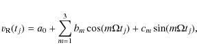
|
(12) |
where the free coefficients a0, bm, and cm are determined by minimizing the chi square between the model and the observations. Specifically, we apply the normal equation method and use LU decomposition and backsubstitution to solve the corresponding set of linear equations for the model coefficients (Press et al. 1992, Sect. 15.4). As in Queloz et al. (2009), we adopt
To check whether our simulated RV curve of CoRoT-7 contains spurious
oscillations at the orbital frequencies of CoRoT-7b or CoRoT-7c, we fit
a trigonometric polynomial of the form
![]() to each residual time series and compute the corresponding semiamplitude
to each residual time series and compute the corresponding semiamplitude
![]() ,
where
,
where
![]() is the orbital frequency of the corresponding planet. In the considered 105 simulations, A is always lower than 0.85 m s-1 at the frequency of CoRoT-7b and lower than 1.7 m s-1 at the frequency of CoRoT-7c. The RV oscillations attributed to CoRoT-7b and CoRoT-7c have semiamplitudes K = 3.5
is the orbital frequency of the corresponding planet. In the considered 105 simulations, A is always lower than 0.85 m s-1 at the frequency of CoRoT-7b and lower than 1.7 m s-1 at the frequency of CoRoT-7c. The RV oscillations attributed to CoRoT-7b and CoRoT-7c have semiamplitudes K = 3.5 ![]() 0.6 and K = 4.0
0.6 and K = 4.0 ![]() 0.5 m s-1, respectively. Therefore, the probability that they come from the residual effects of stellar activity is below 10-4 in both cases.
0.5 m s-1, respectively. Therefore, the probability that they come from the residual effects of stellar activity is below 10-4 in both cases.
Since the amplitude of the light modulation during the HARPS observing season was greater by a factor of ![]() than during CoRoT observations, the activity-induced
RV oscillations are expected to have been greater during those
observations than those simulated from our spot-modelling maps.
Nevertheless, even increasing the amplitudes of the residual
oscillations by a factor of 2, the false alarm probability remains
below 10-4.
than during CoRoT observations, the activity-induced
RV oscillations are expected to have been greater during those
observations than those simulated from our spot-modelling maps.
Nevertheless, even increasing the amplitudes of the residual
oscillations by a factor of 2, the false alarm probability remains
below 10-4.
5.3.2 Constraining the facular area
While our photometric modelling does not exclude a facular-to-spotted area ratio Q > 1, we can constrain it on the basis of the observed RV curve. By computing spot models with Q
ranging from 4 to 10, we find that the peak-to-peak amplitude
of the RV variations increases from 45.7 to
120.3 m s-1 for a lightcurve relative amplitude of 0.0185 and spots located within
![]() from the equator. Given an observed amplitude of
from the equator. Given an observed amplitude of ![]() m s-1 for a photometric relative modulation of
m s-1 for a photometric relative modulation of
![]() ,
we conclude that the amplitude of the observed RV curve can be reproduced only if Q < 4, which is compatible with our adoption of Q=1 corresponding to the minimum of the
,
we conclude that the amplitude of the observed RV curve can be reproduced only if Q < 4, which is compatible with our adoption of Q=1 corresponding to the minimum of the ![]() of the composite photometric best fit. Since the RV amplitude is
dominated by convective redshifts in faculae and spots, it could
be possible to reduce it for
of the composite photometric best fit. Since the RV amplitude is
dominated by convective redshifts in faculae and spots, it could
be possible to reduce it for ![]() by reducing
by reducing
![]() and
and
![]() ,
or decreasing the spot contrast
,
or decreasing the spot contrast ![]() that leads to smaller spots, hence smaller facular areas for a fixed Q. However, the required decrease in
that leads to smaller spots, hence smaller facular areas for a fixed Q. However, the required decrease in
![]() and
and
![]() should be at least of
should be at least of ![]() percent for
percent for ![]() ,
i.e., significantly greater than allowed by the scaling relationship proposed by Gray (2009). Similarly, the required decrease in
,
i.e., significantly greater than allowed by the scaling relationship proposed by Gray (2009). Similarly, the required decrease in ![]() should be too large to be compatible with our assumption of active regions with solar-like contrasts.
should be too large to be compatible with our assumption of active regions with solar-like contrasts.
Our model assumes that the active regions are located close to the
equator, according to the ME prescription that tries to minimize
their area as much as possible. Nevertheless, we also computed a spot
model with Q=6.5 and the constraint that active regions are located at high latitudes (
![]() ),
to study the impact on the RV perturbations. The resulting
RV time series is very similar, with differences never exceeding
),
to study the impact on the RV perturbations. The resulting
RV time series is very similar, with differences never exceeding ![]() m s-1,
to the case of low-latitude spots. This happens because the
reduction in the convective redshifts, due to projection effects,
is compensated by an increase in the continuum flux perturbation
due to the faculae, since they are closer to the limb for most of the
time. In summary, we conclude that a model with Q=1 is appropriate for CoRoT-7, even if its active regions were not constrained to low latitudes.
m s-1,
to the case of low-latitude spots. This happens because the
reduction in the convective redshifts, due to projection effects,
is compensated by an increase in the continuum flux perturbation
due to the faculae, since they are closer to the limb for most of the
time. In summary, we conclude that a model with Q=1 is appropriate for CoRoT-7, even if its active regions were not constrained to low latitudes.
6 Discussion
We analysed the white band lightcurve of the active late-type star CoRoT-7 that hosts a transiting Earth-like planet while a detailed analysis of its RV variations provided evidence of a second non-transiting Earth-like planet (Queloz et al. 2009; Léger et al. 2009). Since the major source of RV variations in CoRoT-7 is stellar magnetic activity, it needs to be modelled in order to refine the planetary orbital parameters and confirm the presence of the second planet CoRoT-7c (Queloz et al. 2009). In principle, the RV oscillation attributed to CoRoT-7c could be spurious and be the effect of stellar activity because its frequency is close to the fifth harmonic of the stellar rotational frequency. Unfortunately, the CoRoT observations are not simultaneous to the RV time series by Queloz et al. (2009) so our conclusions based on modelling CoRoT data do not constrain, rigorously speaking, magnetic activity properties during the RV observations. Nevertheless, we can derive illustrative conclusions from our results, which can be applied to the analysis of the RV time series.
Our favoured spot model has a facular-to-spotted area ratio Q=1,
as expected for a star with an activity level significantly higher
than the Sun. In our simulated RV time series, most of the
power falls at the rotation frequency and its first harmonic. In their
analysis of the observed RV time series of CoRoT-7, Queloz et al. (2009)
find that most of the power falls at the rotation frequency and at
frequencies corresponding to periods of 9.03 and 10.6 days,
the latter corresponding to the first harmonic of the rotation
frequency. Another prominent peak corresponds to a period of
27.6 days (cf. their Table 2). The period of
27.6 days could be associated with the rotation of spots at high
latitudes given that the relative amplitude of the surface differential
rotation of CoRoT-7 is at least ![]() percent. As discussed in Sect. 5.2, a pole-equator angular velocity difference comparable to the Sun, i.e.,
percent. As discussed in Sect. 5.2, a pole-equator angular velocity difference comparable to the Sun, i.e.,
![]() percent,
can indeed be present in our star. This is compatible with a rotation
period of 23.6 days at the equator and of 27.6 days at high
latitudes. The observed peak corresponding to a period of
9.03 days may therefore be the second harmonic of the
high-latitude rotation frequency. Recently, Hatzes et al.
(private comm.) have suggested that such a modulation may be
associated with a third planet. Our approach cannot be applied to
support or disprove this hypothesis because our RV model does not
include the effect of surface differential rotation and high-latitude
active regions that may be producing the 27.6 day periodicity and
its harmonics. Therefore, we have to postpone an investigation of the
role of activity-induced effects for the 9.03 day periodicity to a
future work.
percent,
can indeed be present in our star. This is compatible with a rotation
period of 23.6 days at the equator and of 27.6 days at high
latitudes. The observed peak corresponding to a period of
9.03 days may therefore be the second harmonic of the
high-latitude rotation frequency. Recently, Hatzes et al.
(private comm.) have suggested that such a modulation may be
associated with a third planet. Our approach cannot be applied to
support or disprove this hypothesis because our RV model does not
include the effect of surface differential rotation and high-latitude
active regions that may be producing the 27.6 day periodicity and
its harmonics. Therefore, we have to postpone an investigation of the
role of activity-induced effects for the 9.03 day periodicity to a
future work.
A large facular component (![]() )
is disfavoured in the case of CoRoT-7 because the amplitude of the
RV variation, in this case dominated by convective redshifts
in faculae, would then be too large to be compatible with the
RV observations.
)
is disfavoured in the case of CoRoT-7 because the amplitude of the
RV variation, in this case dominated by convective redshifts
in faculae, would then be too large to be compatible with the
RV observations.
Finally, in the periodogram of the residuals of our ME composite best
fit, there is a significant peak corresponding to a period close to the
orbital period of CoRoT-7c (cf. Fig. 5). This peak is also found in the periodogram of the time series of the residuals of the best fit obtained with the method of Queloz et al. (2009),
so it is not an artifact associated with the
ME regularization. The corresponding RV semiamplitude,
estimated with the method described in Sect. 3.2.2, is ![]() m s-1,
i.e., about one order of magnitude less than the
RV oscillation produced by the planet, so these fluctuations
cannot account for the planetary signature. On the other hand, it
cannot be excluded that those photometric oscillations, with a
semiamplitude of only
m s-1,
i.e., about one order of magnitude less than the
RV oscillation produced by the planet, so these fluctuations
cannot account for the planetary signature. On the other hand, it
cannot be excluded that those photometric oscillations, with a
semiamplitude of only ![]()
![]() 10-5 mag,
could be induced by the interaction of the planet with the stellar
coronal magnetic field or by a perturbation of the stellar dynamo by
the planet, as conjectured by, e.g., Lanza (2008,2009).
10-5 mag,
could be induced by the interaction of the planet with the stellar
coronal magnetic field or by a perturbation of the stellar dynamo by
the planet, as conjectured by, e.g., Lanza (2008,2009).
7 Conclusions
We have applied the spot modelling method introduced by Lanza et al. (2009a,b) to the lightcurve of the planet-hosting star CoRoT-7. After adopting a facular-to-spotted area ratio Q=1,
we find evidence of three persistent active longitudes within which
individual active regions form and decay with lifetimes ranging from a
couple of weeks to a few months. The active longitudes migrate in the
adopted reference frame at different rates, which suggests a surface
differential rotation with a relative amplitude of at least 0.058 ![]() 0.017.
The overall spotted area reaches a maximum of 1.6 percent of the
whole surface if the contrasts of dark spots and faculae are adopted as
solar-like. The residuals of the best fit indicate a population of
small spots with areas of the order of 5
0.017.
The overall spotted area reaches a maximum of 1.6 percent of the
whole surface if the contrasts of dark spots and faculae are adopted as
solar-like. The residuals of the best fit indicate a population of
small spots with areas of the order of 5 ![]() 10-4 of the whole stellar surface that evolve on a typical timescale of
10-4 of the whole stellar surface that evolve on a typical timescale of
![]() days. Moreover, we find an oscillation of the optical flux with a semiamplitude
days. Moreover, we find an oscillation of the optical flux with a semiamplitude ![]()
![]() 10-5 mag with the orbital period of the planet CoRoT-7c.
10-5 mag with the orbital period of the planet CoRoT-7c.
We introduce a model to simulate the apparent RV variations induced by
magnetic activity that includes the effect of surface brightness
inhomogeneities, as well as a reduction in the macroturbulence and
convective blueshifts in active regions. We synthesize a time series
for the RV variations of CoRoT-7 adopting the spot model obtained
from the CoRoT white-band lightcurve and assuming that active regions
have solar-like contrasts and are located within
![]() from the equator. Unfortunately, HARPS and CoRoT observations are not
simultaneous, so any model based on the latter does not rigorously
constrain the observed RV variations. Nevertheless,
an extrapolation of our model matches the observed
RV amplitude.
from the equator. Unfortunately, HARPS and CoRoT observations are not
simultaneous, so any model based on the latter does not rigorously
constrain the observed RV variations. Nevertheless,
an extrapolation of our model matches the observed
RV amplitude.
We fit the RV time series with a linear combination of three sinusoids at the rotation frequency and its first two harmonics, following Queloz et al. (2009, Sect. 4), and confirm that their method is appropriate to filtering out most of the activity-induced RV variations. The residual amplitudes at the orbital periods of the planets CoRoT-7b and CoRoT-7c are used to estimate false-alarm probabilities that the RV oscillations attributed to the planets are spurious effects induced by stellar activity. For both planets we find a false-alarm probability lower than 10-4.
The presence of a third planet with a period of 9.03 days cannot be confirmed by means of our approach because this period could be associated to a harmonic of the signal with a period of 27.6 days, which can be produced by spots at high latitude on a differentially rotating star. We shall consider the effects of surface differential rotation in future models of the RV variations to investigate this issue.
AcknowledgementsThe authors are grateful to an anonymous referee for a careful reading of the manuscript and several suggestions to improve their work. A.F.L. wishes to thank Drs. A.-M. Lagrange, N. Meunier, and M. Desort for interesting discussions. Active star research and exoplanetary studies at INAF-Osservatorio Astrofisico di Catania and Dipartimento di Fisica e Astronomia dell'Università degli Studi di Catania are funded by MIUR (Ministero dell'Istruzione, dell'Università e della Ricerca) and by Regione Siciliana, whose financial support is gratefully acknowledged. This research has made use of the CoRoT Public Data Archive operated at the IAS, Orsay, France, and of the ADS-CDS databases, operated at the CDS, Strasbourg, France.
References
- Alonso, R., Auvergne, M., Baglin, A., et al. 2008, A&A, 482, L21 [NASA ADS] [CrossRef] [EDP Sciences] [Google Scholar]
- Auvergne, M., Bodin, P., Boisnard, L., et al. 2009, A&A, 506, 411 [NASA ADS] [CrossRef] [EDP Sciences] [Google Scholar]
- Baglin, A., Auvergne, M., Boisnard, L., et al. 2006, 36th COSPAR Scientific Assembly, 36, 3749 [Google Scholar]
- Barnes, J. R., Cameron, A. C., Donati, J.-F., et al. 2005, MNRAS, 357, L1 [NASA ADS] [CrossRef] [MathSciNet] [Google Scholar]
- Bruntt, H., Deleuil, M., Fridlund, M., et al. 2010, A&A, 519, A51 [NASA ADS] [CrossRef] [EDP Sciences] [Google Scholar]
- Chapman, G. A., Cookson, A. M., & Dobias, J. J. 1994, ApJ, 432, 403 [NASA ADS] [CrossRef] [Google Scholar]
- Croll, B., Walker, G. A. H., Kuschnig, R., et al. 2006, ApJ, 648, 607 [NASA ADS] [CrossRef] [Google Scholar]
- Desort, M., Lagrange, A.-M., Galland, F., Udry, S., & Mayor, M. 2007, A&A, 473, 983 [NASA ADS] [CrossRef] [EDP Sciences] [Google Scholar]
- Gray, D. F. 1988, Lectures on spectral line analysis: F, G, and K stars (Ontario: Arva) [Google Scholar]
- Gray, D. F. 2009, ApJ, 697, 1032 [NASA ADS] [CrossRef] [Google Scholar]
- Huber, K. F., Wolter, U., Czesla, S., et al. 2009, A&A, 501, 715 [NASA ADS] [CrossRef] [EDP Sciences] [Google Scholar]
- Kurucz, R. L. 2000, http://kurucz.harvard.edu/ [Google Scholar]
- Lagrange, A.-M., Desort, M., & Meunier, N. 2010, A&A, 512, A38 [NASA ADS] [CrossRef] [EDP Sciences] [Google Scholar]
- Lampton, M., Margon, B., & Bowyer, S. 1976, ApJ, 208, 177 [NASA ADS] [CrossRef] [Google Scholar]
- Lanza, A. F. 2008, A&A, 487, 1163 [NASA ADS] [CrossRef] [EDP Sciences] [Google Scholar]
- Lanza, A. F. 2009, A&A, 505, 339 [NASA ADS] [CrossRef] [EDP Sciences] [Google Scholar]
- Lanza, A. F., Catalano, S., Cutispoto, G., Pagano, I., & Rodonò, M. 1998, A&A, 332, 541 [NASA ADS] [Google Scholar]
- Lanza, A. F., Rodonò, M., Pagano, I., Barge, P., & Llebaria, A. 2003, A&A, 403, 1135 [NASA ADS] [CrossRef] [EDP Sciences] [Google Scholar]
- Lanza, A. F., Rodonò, M., & Pagano, I. 2004, A&A, 425, 707 [NASA ADS] [CrossRef] [EDP Sciences] [Google Scholar]
- Lanza, A. F., Bonomo, A. S., & Rodonò, M. 2007, A&A, 464, 741 [NASA ADS] [CrossRef] [EDP Sciences] [Google Scholar]
- Lanza, A. F., Pagano, I., Leto, G., et al. 2009a, A&A, 493, 193 [NASA ADS] [CrossRef] [EDP Sciences] [Google Scholar]
- Lanza, A. F., Aigrain, S., Messina, S., et al. 2009b, A&A, 506, 255 [NASA ADS] [CrossRef] [EDP Sciences] [Google Scholar]
- Léger, A., Rouan, D., Schneider, J., et al. 2009, A&A, 506, 287 [NASA ADS] [CrossRef] [EDP Sciences] [MathSciNet] [Google Scholar]
- Lockwood, G. W., Skiff, B. A., Henry, G. W., et al. 2007, ApJS, 171, 260 [NASA ADS] [CrossRef] [Google Scholar]
- Lomb, N. R. 1976, Ap&SS, 39, 447 [NASA ADS] [CrossRef] [Google Scholar]
- Meunier, N., Desort, M., & Lagrange, A.-M. 2010, A&A, 512, A39 [NASA ADS] [CrossRef] [EDP Sciences] [Google Scholar]
- Press, W. H., Teukolsky, S. A., Vetterling, W. T., & Flannery, B. P. 1992, Numerical Recipes, 2nd edn. (Cambridge: Cambridge Univ. Press) [Google Scholar]
- Queloz, D., Henry, G. W., Sivan, J. P., et al. 2001, A&A, 379, 279 [NASA ADS] [CrossRef] [EDP Sciences] [Google Scholar]
- Queloz, D., Bouchy, F., Moutou, C., et al. 2009, A&A, 506, 303 [NASA ADS] [CrossRef] [EDP Sciences] [Google Scholar]
- Radick, R. R., Lockwood, G. W., Skiff, B. A., & Baliunas, S. L. 1998, ApJS, 118, 239 [NASA ADS] [CrossRef] [Google Scholar]
- Saar, S. H., & Donauhe, R. A. 1997, ApJ, 485, 319 [NASA ADS] [CrossRef] [Google Scholar]
- Saar, S. H., Butler, R. P., & Marcy, G. W. 1998, ApJ, 498, L153 [Google Scholar]
- Scargle, J. D. 1982, ApJ, 263, 835 [NASA ADS] [CrossRef] [Google Scholar]
- Strassmeier, K. G. 2009, A&ARv, 17, 251 [NASA ADS] [CrossRef] [Google Scholar]
- Title, A. M., Topka, K. P., Tarbell, T. D., et al. 1992, ApJ, 393, 782 [NASA ADS] [CrossRef] [Google Scholar]
- Vogt, S. S., & Penrod, G. D. 1983, PASP, 95, 565 [NASA ADS] [CrossRef] [Google Scholar]
Footnotes
- ... CoRoT-7
- Based on observations obtained with CoRoT, a space project operated by the French Space Agency, CNES, with partecipation of the Science Programme of ESA, ESTEC/RSSD, Austria, Belgium, Brazil, Germany, and Spain.
All Tables
Table 1: Parameters adopted for the lightcurve and RV modelling of CoRoT-7.
All Figures
|
|
Figure 1: Apparent RV variation (upper panel) and relative stellar flux (lower panel) vs. the rotation phase produced by a single active region on a star seen equator-on. Different linestyles indicate different kinds of inhomogeneities inside the active region. Dashed: reduced macroturbulence without brightness perturbation; solid: dark spot and reduced macroturbulence; dotted: dark spot, bright facula, and reduced macroturbulence. The flux is measured in units of the unperturbed stellar flux. |
| Open with DEXTER | |
| In the text | |
|
|
Figure 2: Same as Fig. 1 when including (solid line) and not including (dotted line) the convective redshifts in cool spots and bright faculae in the simulation (see the text for the active region parameters). |
| Open with DEXTER | |
| In the text | |
|
|
Figure 3:
The ratio of the |
| Open with DEXTER | |
| In the text | |
|
|
Figure 4:
Upper panel: the out-of-transit lightcurve of CoRoT-7 (dots) and its ME-regularized best fit for a facular-to-spotted area ratio of Q=1.0
(solid line). The flux is normalized to the maximum observed flux. The
vertical dashed lines mark the individually fitted intervals of
|
| Open with DEXTER | |
| In the text | |
|
|
Figure 5:
Lomb-Scargle periodogram of the residual time series of Fig. 4. The dashed horizontal line marks a false-alarm probability of 10-6. The vertical dot-dashed lines mark the orbital frequencies of the planets CoRoT-7b (right,
|
| Open with DEXTER | |
| In the text | |
|
|
Figure 6:
Distributions of the spotted area vs. longitude during the time intervals centred on the labelled times (
|
| Open with DEXTER | |
| In the text | |
|
|
Figure 7: The total spotted area as derived from our lightcurve model illustrated in Figs. 4 and 6. The uncertainty of the area has been estimated from the errors of the photometric observations. |
| Open with DEXTER | |
| In the text | |
|
|
Figure 8: Upper panel: the synthesized RV variation due to stellar active regions vs. time as derived from our ME spot modelling with Q=1 (solid line) and Q=0 (dotted line). To illustrate the effect of an examplary ground-based sampling, open diamonds mark the times of HARPS observations by Queloz et al. (2009) after shifting their initial epoch to ten days after the beginning of CoRoT observations. Lower panel: the synthesized relative flux variation in the CoRoT white passband vs. time (solid line) with HARPS time sampling marked by open diamonds. |
| Open with DEXTER | |
| In the text | |
|
|
Figure 9: The average Lomb periodogram of 105 synthetic RV time series vs. frequency (solid line) and the average periodogram obtained after filtering the series with the three-harmonic model of Queloz et al. (2009) (dashed line). The power is normalized to the maximum value of the unfiltered mean periodogram. The dot-dashed lines mark the rotation frequency, its first, and second harmonics, while the three-dot-dashed lines mark the orbital frequencies of CoRoT-7c (left) and CoRoT-7b (right), respectively. |
| Open with DEXTER | |
| In the text | |
Copyright ESO 2010
Current usage metrics show cumulative count of Article Views (full-text article views including HTML views, PDF and ePub downloads, according to the available data) and Abstracts Views on Vision4Press platform.
Data correspond to usage on the plateform after 2015. The current usage metrics is available 48-96 hours after online publication and is updated daily on week days.
Initial download of the metrics may take a while.