| Issue |
A&A
Volume 520, September-October 2010
|
|
|---|---|---|
| Article Number | A36 | |
| Number of page(s) | 10 | |
| Section | Extragalactic astronomy | |
| DOI | https://doi.org/10.1051/0004-6361/201014091 | |
| Published online | 27 September 2010 | |
XMM-Newton RGS observation of the warm absorber in Mrk 279
J. Ebrero1 - E. Costantini1 - J. S. Kaastra1,2 - R. G. Detmers1 - N. Arav3 - G. A. Kriss4 - K. T. Korista5 - K. C. Steenbrugge6,7
1 - SRON Netherlands Institute for Space Research, Sorbonnelaan 2, 3584 CA, Utrecht, The Netherlands
2 -
Astronomical Institute, University of Utrecht, Postbus 80000, 3508 TA, Utrecht, The Netherlands
3 -
Department of Physics, Virginia Tech, Blacksburg, VA 24061, USA
4 -
Space Telescope Science Institute, 3700 San Martin Drive, Baltimore, MD 21218, USA
5 -
Department of Physics, Western Michigan University, Kalamazoo, MI 49008, USA
6 -
Instituto de Astronomía, Universidad Católica del Norte, Avenida Angamos 0610, Casilla 1280, Antofagasta, Chile
7 -
University of Oxford, Department of Physics, Keble Road, OX1 3RH, Oxford, UK
Received 18 January 2010 / Accepted 3 June 2010
Abstract
Context. The Seyfert 1 galaxy Mrk 279 was observed by XMM-Newton in November 2005 on three consecutive orbits, showing significant short-scale variability (average soft band variation in flux ![]() 20%). The source is known to host a two-component warm absorber with distinct ionisation states from a previous Chandra observation.
20%). The source is known to host a two-component warm absorber with distinct ionisation states from a previous Chandra observation.
Aims. We study the warm absorber in Mrk 279 and investigate any
possible response to the short-term variations in the ionising flux and
assess whether it has varied on a long-term timescale with respect to
the Chandra observation.
Methods. The XMM-Newton-RGS spectra of Mrk 279 were analysed in both the high- and low-flux states using the SPEX fitting package.
Results. We find no significant changes in the warm absorber on either short timescales (![]() 2
days) or longer ones (two and a half years), as the variations in the
ionic column densities of the most relevant elements are below the 90%
confidence level. The variations could still be present but are
statistically undetected given the signal-to-noise ratio of the data.
Starting from reasonable standard assumptions, we estimate the location
of the absorbing gas, which is likely to be associated with the
putative dusty torus rather than with the broad line region if the
outflowing gas is moving at the escape velocity or greater.
2
days) or longer ones (two and a half years), as the variations in the
ionic column densities of the most relevant elements are below the 90%
confidence level. The variations could still be present but are
statistically undetected given the signal-to-noise ratio of the data.
Starting from reasonable standard assumptions, we estimate the location
of the absorbing gas, which is likely to be associated with the
putative dusty torus rather than with the broad line region if the
outflowing gas is moving at the escape velocity or greater.
Key words: galaxies: individual: Mrk 279 - galaxies: Seyfert - quasars: absorption lines - X-rays: galaxies
1 Introduction
It is widely believed that active galactic nuclei (AGN) are powered by gravitational accretion of matter onto the supermassive black hole that resides in their centres (see e.g. Rees 1984, for a review). X-ray emission, characteristic of AGN activity, is therefore a fundamental tracer of the accretion processes that take place in the innermost regions of the AGN engine.
More than 50% of the Seyfert 1 galaxies exhibit clear signatures of a photoionised gas, the so-called warm absorber (WA hereafter, Reynolds 1997; George et al. 1998), in their X-ray spectra in the form of narrow absorption features, usually blueshifted by a few hundred km s-1, thus revealing the presence of outflows from the nucleus along the line of sight (Crenshaw et al. 1999; Kaastra et al. 2000; Kaspi et al. 2001; Kaastra et al. 2002). The study of warm absorbers provides unique insight into the innermost AGN environment, allowing us to probe elemental abundances, degrees of ionisation, outflow velocities, among others.
However, the geometrical structure and origin of the WA, its physical connection with the continuum emission source, and other components of the AGN, such as the broad line region (BLR), narrow line region (NLR), and the putative dusty torus, are not yet clear. A number of theories have been proposed to explain the origin of WA such as evaporation from the torus (Krolik & Kriss 2001), outflowing winds from the accretion disc (e.g. Murray & Chiang 1995; Elvis 2000), or the ionisation cone theory (Kinkhabwala et al. 2002). The study of Blustin et al. (2005) on 23 AGN suggests that the WA in most of the nearby Seyfert galaxies is likely to originate in outflows from the molecular torus.
The main problem for determining the distance between the WA
and the ionising source comes from the fact that the determination of
the ionisation parameter of the gas and the ionising luminosity from a
single time-averaged observation only allows the product
![]() to be derived. This degeneracy of the electron density
to be derived. This degeneracy of the electron density ![]() and the distance R
can be broken by measuring the variations in the ionisation state of
the gas in response to changes in the ionising continuum. Therefore,
the density of the gas can be measured and its distance from the source
determined (e.g. NGC 3516, Netzer et al. 2002).
Studies of variability of the WA have been carried out only in a
handful of objects on timescales of a few ks (e.g. MCG-6-30-15, Gibson
et al. 2007; Miller et al. 2008; NGC 4051, Krongold et al. 2007; NGC 1365, Risaliti et al. 2009) and also on longer timescales (e.g. NGC 5548, Krongold et al. 2010).
and the distance R
can be broken by measuring the variations in the ionisation state of
the gas in response to changes in the ionising continuum. Therefore,
the density of the gas can be measured and its distance from the source
determined (e.g. NGC 3516, Netzer et al. 2002).
Studies of variability of the WA have been carried out only in a
handful of objects on timescales of a few ks (e.g. MCG-6-30-15, Gibson
et al. 2007; Miller et al. 2008; NGC 4051, Krongold et al. 2007; NGC 1365, Risaliti et al. 2009) and also on longer timescales (e.g. NGC 5548, Krongold et al. 2010).
Mrk 279 is a nearby (z=0.0305, Scott et al. 2004) Seyfert 1 galaxy (
![]() erg cm-2 s-1, this work). The source was previously observed in X-rays by the HEAO 1 A-2 experiment (Weaver et al. 1995) and ASCA (Weaver et al. 2001) in order to study the spectral complexity of the Fe K
erg cm-2 s-1, this work). The source was previously observed in X-rays by the HEAO 1 A-2 experiment (Weaver et al. 1995) and ASCA (Weaver et al. 2001) in order to study the spectral complexity of the Fe K![]() emission line region. More recently, Mrk 279 has been observed in X-rays using Chandra-HETGS simultaneously with FUSE and HST-STIS in 2002 (Scott et al. 2004).
They found strong complex absorption features from both high- and
low-ionisation elements in the UV spectrum but no hints of absorption
in the X-ray band due to the low continuum flux at the moment of the
observation. In 2003 the source was observed again by FUSE, HST-STIS (Gabel et al. 2005), and LETGS onboard Chandra (Costantini et al. 2007).
They quantified the contribution of the BLR to the soft X-ray spectrum,
via the locally optimally emitting clouds (LOC) model (Baldwin
et al. 1995), and determined that the broad lines observed at soft X-rays were consistent with a BLR origin.
emission line region. More recently, Mrk 279 has been observed in X-rays using Chandra-HETGS simultaneously with FUSE and HST-STIS in 2002 (Scott et al. 2004).
They found strong complex absorption features from both high- and
low-ionisation elements in the UV spectrum but no hints of absorption
in the X-ray band due to the low continuum flux at the moment of the
observation. In 2003 the source was observed again by FUSE, HST-STIS (Gabel et al. 2005), and LETGS onboard Chandra (Costantini et al. 2007).
They quantified the contribution of the BLR to the soft X-ray spectrum,
via the locally optimally emitting clouds (LOC) model (Baldwin
et al. 1995), and determined that the broad lines observed at soft X-rays were consistent with a BLR origin.
This paper is devoted to the XMM-Newton-RGS spectra of Mrk 279. The XMM-Newton-EPIC broad band analysis is presented in a companion paper (Costantini et al. 2010, Paper I hereafter). It is organised as follows. In Sect. 2 we describe the X-ray datasets used in this study. In Sect. 3 we describe the spectral analysis of the most relevant features, while in Sect. 4 we discuss our results. Finally, our conclusions are reported in Sect. 5.
Throughout this paper we have assumed a cosmological framework with H0=70 km s-1 Mpc-1,
![]() and
and
![]() (Spergel at al. 2003). The quoted errors refer to 68.3% confidence level (
(Spergel at al. 2003). The quoted errors refer to 68.3% confidence level (
![]() for one parameter of interest) unless otherwise stated.
for one parameter of interest) unless otherwise stated.
2 The X-ray data
Mrk 279 was observed by XMM-Newton on three consecutive orbits between November 15 and November 19, 2005 for a total of ![]() 160 ks. The RGS data were processed using the standard pipeline SAS v9.0 (Gabriel et al. 2004). After filtering background flaring events, the RGS total net exposure time is
160 ks. The RGS data were processed using the standard pipeline SAS v9.0 (Gabriel et al. 2004). After filtering background flaring events, the RGS total net exposure time is ![]() 110 ks. A summary of the observation log is reported in Table 1, and the lightcurve of the three observations is shown in Fig. 1.
110 ks. A summary of the observation log is reported in Table 1, and the lightcurve of the three observations is shown in Fig. 1.
Table 1: XMM- Newton observation log.
![\begin{figure}
\par\includegraphics[angle=90,width=9cm,clip]{14091fg1.ps}
\end{figure}](/articles/aa/full_html/2010/12/aa14091-10/img15.png)
|
Figure 1: EPIC-pn lightcurve in the 0.3-2 keV band. |
| Open with DEXTER | |
It can be seen from Fig. 1 that the source experienced strong variations in flux on a relatively short timescale, which is especially clear in the plotted 0.3-2 keV band, where we find a maximal variation in flux of about 20% between orbits 1087 and 1088. The source flux recovered during orbit 1089 so that its brightness was comparable to that of orbit 1087 by the end of the observation. For clarity, in what follows the 1087-, 1088-, and 1089-orbit, RGS datasets will be labeled as high (H), low (L), and recovering (R), respectively, according to their relative flux state.
For the purpose of this study, the R dataset was included in the overall fit described in Sect. 3
in order to increase the statistics. However, since we are interested
in investigating the possible spectral variations in two clearly
distinct flux states, we mainly focus on the H and L
datasets. In all datasets under study, RGS1 and RGS2 were analysed
together. We used C-statistics during the spectral analysis (see
Sect. 3) so that binning of
the data is in theory no longer needed. However, to avoid oversampling,
we rebinned the data by a factor of 3. The signal-to-noise ratio for
both datasets is around ![]() 9 and
9 and ![]() 8 for H and L, respectively, for that part of the wavelength region in which the most relevant spectral features fall.
8 for H and L, respectively, for that part of the wavelength region in which the most relevant spectral features fall.
3 Spectral analysis with RGS
The spectral analysis of the RGS data was carried out with the fitting package SPEX![]() v2.0 (Kaastra et al. 1996). Both RGS1 and RGS2 were fitted together, and C-statistics was the fitting method adopted (Cash 1979). The same spectral model was applied to H, L, and R datasets, and they were fitted simultaneously using three different sectors in SPEX.
The advantage of assigning a sector to each dataset under study resides
in the fact that, although some of the parameters might be different in
general (e.g. the continuum parameters), it allows parameters from
different datasets to be coupled and fitted simultaneously (see SPEX documentation for further information). The final C-stat/d.o.f. = 4857/
v2.0 (Kaastra et al. 1996). Both RGS1 and RGS2 were fitted together, and C-statistics was the fitting method adopted (Cash 1979). The same spectral model was applied to H, L, and R datasets, and they were fitted simultaneously using three different sectors in SPEX.
The advantage of assigning a sector to each dataset under study resides
in the fact that, although some of the parameters might be different in
general (e.g. the continuum parameters), it allows parameters from
different datasets to be coupled and fitted simultaneously (see SPEX documentation for further information). The final C-stat/d.o.f. = 4857/
![]() obtained applies to the final simultaneous fit of all three datasets.
In what follows we describe the continuum and the absorption and
emission features that are present in the spectrum of Mrk 279.
obtained applies to the final simultaneous fit of all three datasets.
In what follows we describe the continuum and the absorption and
emission features that are present in the spectrum of Mrk 279.
3.1 Continuum spectrum
The broadband (0.3-10 keV) continuum spectrum of Mrk 279 is best described by a broken power law and a black body (see Paper I). In the soft X-rays region (0.3-2 keV), however, a single power law provides a good description of the baseline continuum, although deviations exist at very soft X-rays (soft excess).
To account for the soft excess we added a modified black body model (mbb model in SPEX)
to the power law, which considers modifications of a simple black body
by coherent Compton scattering and is based on the calculations of
Kaastra & Barr (1989). The improvement of the fit after adding this component was
![]() for 6 degrees of freedom.
for 6 degrees of freedom.
The best-fit parameters of the continuum are reported in Table 2 for the H, L, and R datasets. The slope ![]() seems slightly steeper when the source is in the high-flux state,
although this value is consistent within the error bars with the value
determined for the low-flux state. The value obtained for the R
dataset lies in between the former, and it is still consistent within
the error bars. The thermal component remains virtually unchanged in
all three datasets.
seems slightly steeper when the source is in the high-flux state,
although this value is consistent within the error bars with the value
determined for the low-flux state. The value obtained for the R
dataset lies in between the former, and it is still consistent within
the error bars. The thermal component remains virtually unchanged in
all three datasets.
3.2 Absorption at redshift zero
The continuum emission of Mrk 279 is furrowed by several absorption
features, some of them consistent with absorption at redshift zero,
revealing a complex absorption spectrum. The local absorbing gas seems
to have two distinct components: a neutral or mildly ionised absorber,
characterised by the O I feature at ![]() 23.5 Å, with a column density of
23.5 Å, with a column density of
![]() cm-2 (Elvis et al. 1989), and an ionised component with
cm-2 (Elvis et al. 1989), and an ionised component with
![]() cm-2 and
cm-2 and
![]() eV (Costantini et al. 2007).
eV (Costantini et al. 2007).
We modelled these components by means of a collisionally ionised plasma (hot model in SPEX) fixing their parameters to the values listed above. The ionised component likely originates in the interstellar medium of our Galaxy, but an extragalactic origin cannot be ruled out (Nicastro et al. 2002). Further discussion of the absorbing gas along the line of sight of Mrk 279 can be found in Williams et al. (2006).
Table 2: Mrk 279 RGS continuum best-fit parameters.
3.3 The warm absorber
The spectrum of Mrk 279 shows a number of absorption features in the range ![]() 10-35 Å consistent
with the presence of outflowing ionised gas at the redshift of the
source. Previous observations of Mrk 279 with Chandra have
already shown that the absorbing gas consists of at least two phases
with distinct ionisation degrees (Costantini et al. 2007).
10-35 Å consistent
with the presence of outflowing ionised gas at the redshift of the
source. Previous observations of Mrk 279 with Chandra have
already shown that the absorbing gas consists of at least two phases
with distinct ionisation degrees (Costantini et al. 2007).
We therefore modelled the absorption spectrum using two xabs components in SPEX. This model calculates the transmission of a slab of material where all ionic column densities are linked through a photoionisation balance model, which was calculated with CLOUDY (Ferland et al. 1998) version C08. The input spectral energy distribution (SED) of Mrk 279 provided to CLOUDY was based on the Chandra observation carried out in 2003, as the values obtained in the X-ray domain by both Chandra and the current XMM-Newton observation are virtually the same (see Fig. 2). The mean velocity dispersion of the absorption lines was fixed to 50 km s-1 (Costantini et al. 2007).
The addition of one xabs component improves the fit by
![]() for 3 degrees of freedom but fails to reproduce the O VIII Ly
for 3 degrees of freedom but fails to reproduce the O VIII Ly![]() line. A second xabs component is therefore required, improving the fit by a further
line. A second xabs component is therefore required, improving the fit by a further
![]() .
This model consisting of two xabs components with distinct ionisation states provides a good fit to the observed data (see Fig. 4).
.
This model consisting of two xabs components with distinct ionisation states provides a good fit to the observed data (see Fig. 4).
![\begin{figure}
\par\hbox{
\includegraphics[width=6.5cm,angle=90.]{14091fg2.ps} }\end{figure}](/articles/aa/full_html/2010/12/aa14091-10/img37.png)
|
Figure 2: Average spectral energy distribution of Mrk 279. The X-ray continuum is determined by Chandra (crosses, Costantini et al. 2007). For comparison, we overplot the average continuum measured by XMM- Newton (diamonds). For the far UV we relied on the HST and FUSE measurements. |
| Open with DEXTER | |
![\begin{figure}
\par\includegraphics[height=15cm,width=5.5cm,angle=90.]{14091fg3a...
...}
\includegraphics[height=15cm,width=5.5cm,angle=90.]{14091fg3b.ps}
\end{figure}](/articles/aa/full_html/2010/12/aa14091-10/img38.png)
|
Figure 3: RGS spectrum of Mrk 279. For plotting purposes all three observations have been stacked into a single spectrum. The solid line corresponds to the best-fit model. The most relevant spectral features are labelled. |
| Open with DEXTER | |
Table 3: Best-fit xabs parameters to the warm absorber of Mrk 279.
We first fitted the WA in the H, L, and R
datasets independently. If the variations in flux observed between the
first two observations were propagated into the surrounding material,
the ionisation properties of the gas should have changed accordingly.
The results of the fits, however, show that no significant changes took
place in the properties of the WA between the H and L flux states, as most of the parameters are consistent with each other within the error bars (see Table 3). Furthermore, we have normalised the L dataset to the unabsorbed continuum of the H
dataset. In this way we get rid of any possible spectral effects caused
by the change in flux between both observations so that only the
information on the absorption features remains (see e.g. Netzer
et al. 2003). We can see in Fig. 5
that the oxygen complex, as well as the most relevant iron absorption
features, remains virtually unchanged. The physical implications of
this lack of response of the WA to the changes in the ionising flux
between two consecutive observations is discussed further in Sect. 4. We must note, however, that, although the variation in the average flux is ![]() 20%, the uncertainties in
20%, the uncertainties in ![]() are
are ![]() 50%
in the case of the lowest ionisation component. We cannot therefore
discard the possibility that short-scale variability did actually occur
but is undetected statistically.
50%
in the case of the lowest ionisation component. We cannot therefore
discard the possibility that short-scale variability did actually occur
but is undetected statistically.
The results of the fits on the individual observations are reported in Table 3. The WA is clearly present, but its very shallow column density (![]()
![]() cm-2 and
cm-2 and ![]()
![]() cm-2
for low and high ionised WA phases, respectively, in agreement with
previous measurements) makes it rather difficult to detect. This is
especially problematic in the L dataset, where the low flux
level makes some of the absorption troughs almost undetectable, which
is reflected in the larger error bars than in the H dataset. The ionisation parameter
cm-2
for low and high ionised WA phases, respectively, in agreement with
previous measurements) makes it rather difficult to detect. This is
especially problematic in the L dataset, where the low flux
level makes some of the absorption troughs almost undetectable, which
is reflected in the larger error bars than in the H dataset. The ionisation parameter ![]() of the high-ionisation phase seems to be surprisingly stable throughout
the observations, seemingly insensitive to the flux variations of the
source, although its value becomes rather uncertain in the L dataset. Both WA phases seem to be outflowing at different velocities (
of the high-ionisation phase seems to be surprisingly stable throughout
the observations, seemingly insensitive to the flux variations of the
source, although its value becomes rather uncertain in the L dataset. Both WA phases seem to be outflowing at different velocities (![]() 200 km s-1 and
200 km s-1 and ![]() 400 km s-1), with the high-ionisation phase having a faster outflow. The fit to the R
dataset alone was severely affected by the low statistics due to the
short exposure time, and it provided results consistent with those
obtained for the H and L datasets, albeit with much larger error bars.
400 km s-1), with the high-ionisation phase having a faster outflow. The fit to the R
dataset alone was severely affected by the low statistics due to the
short exposure time, and it provided results consistent with those
obtained for the H and L datasets, albeit with much larger error bars.
Since the WA parameters in all datasets were consistent within the error bars, we assumed that the WA was formally under the same physical conditions in both the high and low flux states. Therefore, we fitted again all three datasets coupling this time the H, L and R xabs parameters to each other in order to reduce the associated error on the parameters under consideration. The result of this fit is also reported in Table 3 and it will be the one we will use throughout this paper as a description of the WA in further calculations. This fit is also shown in Fig. 3 where, for plotting purposes, we have stacked the spectra of all three observations. The spectra displayed in Fig. 3 and the following figures were produced by dividing the photon spectra by the effective area of the detector so that no model-dependent fluxing was applied.
![\begin{figure}
\par\includegraphics[angle=90,width=9cm,clip]{14091fg4.ps}
\end{figure}](/articles/aa/full_html/2010/12/aa14091-10/img65.png)
|
Figure 4: Detail of the O VIII absorption line. Overplotted is the fit with only one xabs component (dashed line) and two xabs components (solid line). |
| Open with DEXTER | |
![\begin{figure}
\par\includegraphics[angle=90,width=9cm,clip]{14091fg5.ps}
\end{figure}](/articles/aa/full_html/2010/12/aa14091-10/img66.png)
|
Figure 5: Comparison between the H (black crosses) and L (light stars) datasets. The L dataset is normalised to the unabsorbed continuum of the H dataset. |
| Open with DEXTER | |
3.4 Emission lines
In addition to the absorption features present in the soft X-ray
spectrum of Mrk 279, there are also hints of emission features.
Costantini et al. (2007) reported several narrow emission features of different elements and radiative recombination continua of C V and C VI found in the Chandra-LETG
spectrum of Mrk 279. We were unable to detect most of these lines in
the RGS datasets. We find marginal detection of the O VIII Ly![]() and O VII (forbidden) emission lines in the L dataset, whereas in the H dataset the higher continuum level swamps out these low-significance emission lines (see Table 5).
and O VII (forbidden) emission lines in the L dataset, whereas in the H dataset the higher continuum level swamps out these low-significance emission lines (see Table 5).
At the position of the O VII triplet there
is a weak broad emission line intrinsic to the source. The presence of
this broad line was taken into account while fitting the spectrum of
Mrk 279 by adding a Gaussian line to the model. The line is only
marginally detected at the 90% confidence level in the H and R datasets, whereas it is not significantly detected at all in the L
dataset (see Paper I for a detailed discussion). The complexities
in this spectral range due to bad pixels and the O V, O VI, and O VII absorption lines are such that the significant detection of the O VII
broad line is difficult, considering the signal-to-noise ratio of the
spectra. The origin of this line is likely the BLR, and its luminosity
can be accounted for by the LOC model (Baldwin et al. 1995). Further discussion of this broad feature and how it could be linked to the complex Fe K![]() region of Mrk 279 is given in Paper I.
region of Mrk 279 is given in Paper I.
We used the O VII forbidden emission
line and the upper limits of the other emission lines, which provide
mild constraints, to calculate the emission spectrum of the
two-component WA (see Sect. 3.3) and potentially link the observed emission and absorption. For this, we used CLOUDY and assumed a gas with a density of 108 cm-3.
In this way, the slab of material remains geometrically thin relative
to its distance from the central source. For the purpose of this
calculation we used a covering factor of
![]() ,
defined as the fraction of
,
defined as the fraction of ![]() sr
covered by the gas as viewed from the central ionising source, i.e. the
solid angle subtended by the gas. This is different from the global
covering factor, which is the fraction of emission intercepted by the
absorber averaged over all lines of sight, and it has been estimated to
be about 0.5 (Crenshaw et al. 2003).
sr
covered by the gas as viewed from the central ionising source, i.e. the
solid angle subtended by the gas. This is different from the global
covering factor, which is the fraction of emission intercepted by the
absorber averaged over all lines of sight, and it has been estimated to
be about 0.5 (Crenshaw et al. 2003).
![\begin{figure}
\par\includegraphics[angle=90,width=9cm,clip]{14091fg6.ps}
\end{figure}](/articles/aa/full_html/2010/12/aa14091-10/img68.png)
|
Figure 6:
Emission line contribution of the warm absorbers in Mrk 279, assuming a covering fraction
|
| Open with DEXTER | |
Table 4: Column densitity and outflow velocity of the most relevant X-ray absorption lines.
In Fig. 6 we display our results. Both low- and high-ionisation gas components tend to overestimate the measured luminosities for
![]() .
This is especially clear for the high-
.
This is especially clear for the high-![]() component, while it is less significant in the case of the low-
component, while it is less significant in the case of the low-![]() component. However, the line luminosity scales linearly with
component. However, the line luminosity scales linearly with ![]() in practice (not true for high column densities, when the dependence on
in practice (not true for high column densities, when the dependence on ![]() is more complicated, but it is valid for shallow NH such as the ones found in this source, Netzer 1993, 1996). As the O VII
flux predicted by the high-ionisation component is approximately three
times the flux of the low-ionisation gas, the scaling of the
predicted-to-observed O VII luminosity is dominated by the high-ionisation gas. If a single component were to explain the O VII forbidden line, an
is more complicated, but it is valid for shallow NH such as the ones found in this source, Netzer 1993, 1996). As the O VII
flux predicted by the high-ionisation component is approximately three
times the flux of the low-ionisation gas, the scaling of the
predicted-to-observed O VII luminosity is dominated by the high-ionisation gas. If a single component were to explain the O VII forbidden line, an ![]() of 0.4 and 0.13 would be needed for the low- and high-ionisation gas,
respectively, whereas for a combination of both components a
of 0.4 and 0.13 would be needed for the low- and high-ionisation gas,
respectively, whereas for a combination of both components a
![]() is required to match the luminosities predicted by CLOUDY
with the observed ones. This is in tune with what is found for
unobscured or Compton-thin AGN, where absorption lines are more
dominant than the emission lines in cases in which a cloud, belonging
to a population of clouds with a low global covering factor, happens to
lie along the line of sight of the observer. In this case the emission
lines coming from other directions provide a negligible contribution to
the total spectrum (Nicastro et al. 1999; Bianchi et al. 2005).
is required to match the luminosities predicted by CLOUDY
with the observed ones. This is in tune with what is found for
unobscured or Compton-thin AGN, where absorption lines are more
dominant than the emission lines in cases in which a cloud, belonging
to a population of clouds with a low global covering factor, happens to
lie along the line of sight of the observer. In this case the emission
lines coming from other directions provide a negligible contribution to
the total spectrum (Nicastro et al. 1999; Bianchi et al. 2005).
In Fig. 6 we also plot the sum of the components scaled to the luminosity of the O VII
line. We see that the normalised model is in agreement with the upper
limits of the lower ionisation lines. We also note that none of the gas
components that produce absorption are sufficient to produce the Fe K![]() narrow component in emission that is detected in the pn spectrum (see Paper I), where the total contribution is
narrow component in emission that is detected in the pn spectrum (see Paper I), where the total contribution is ![]() 0.5%.
0.5%.
Table 5: Emission line luminosities measured by RGS and their significance.
4 Discussion
4.1 Two ionisation components in the warm absorber
The absorption features detected in the spectrum of Mrk 279 are
consistent with those produced by different elements, mainly oxygen,
carbon, nitrogen, and iron, with different degrees of ionisation. These
troughs are blueshifted with respect to the systemic velocity of the
source, and their degree of ionisation reveals that they are associated
with a WA often seen in other Seyfert 1 galaxies. The absorbing gas
presents at least two phases with ionisation parameters of
![]() and
and
![]() ,
respectively, and quite low
,
respectively, and quite low ![]() (
(![]() 1020 cm-2, see Table 3).
1020 cm-2, see Table 3).
The question about whether the outflowing gas forms clouds in
equilibrium with its surroundings or if it is part of a continuous
distribution of ionised material is difficult to answer in the case of
Mrk 279. In the first case, the clouds should be in pressure
equilibrium with the less dense environment to allow for long-lived
structures. Such a scenario has been already claimed in the case of the
Seyfert 1 galaxy NGC 3783 (Krongold et al. 2003; Netzer et al. 2003; Krongold et al. 2005).
If the WA components indeed belong to a discrete scenario with a sharp
bimodal distribution, then their pressure ionisation parameter ![]() should be the same, where
should be the same, where ![]() can be defined as a function of pressure or temperature:
can be defined as a function of pressure or temperature:
![]() .
If we overplot the values of
.
If we overplot the values of ![]() corresponding to the two phases of the WA detected in Mrk 279 on the
corresponding to the two phases of the WA detected in Mrk 279 on the ![]() curve of the source we can see that both components cannot be in
pressure equilibrium unless other processes such as magnetic
confinement are playing a role (see Fig. 7). Similar results were also found in the Chandra analysis of Mrk 279 (Costantini et al. 2007).
curve of the source we can see that both components cannot be in
pressure equilibrium unless other processes such as magnetic
confinement are playing a role (see Fig. 7). Similar results were also found in the Chandra analysis of Mrk 279 (Costantini et al. 2007).
![\begin{figure}
\par\includegraphics[angle=-90,width=9cm,clip]{14091fg7.ps}\end{figure}](/articles/aa/full_html/2010/12/aa14091-10/img100.png)
|
Figure 7: Pressure ionisation parameter as a function of electron temperature. The values corresponding to the warm absorber components in Mrk 279 are marked as squares. |
| Open with DEXTER | |
![\begin{figure}
\par\mbox{\includegraphics[width=6.5cm,angle=-90]{14091fg8a.ps}\i...
...091fg8c.ps}\includegraphics[width=6.5cm,angle=-90]{14091fg8d.ps} }\end{figure}](/articles/aa/full_html/2010/12/aa14091-10/img101.png)
|
Figure 8:
Ionic column densities of Fe (upper left panel), Ne (upper right panel), C (lower left panel), and O (lower right panel) ions in the XMM- Newton (solid lines, this work; dots: low- |
| Open with DEXTER | |
4.2 Is the warm absorber variable?
Mrk 279 is known for experiencing moderate flux variability on timescales of a few tens of ks (Scott et al. 2004; Costantini et al. 2010). If these changes in the ionising flux were to produce any measurable changes in the physical conditions of the absorbing gas on both short and long timescales, they could in principle be used to estimate the location of the absorber.
The XMM-Newton lightcurve of Mrk 279 in the 0.3-2 keV range looked promising in this respect, since we observe a flux variation of ![]() 20% between the H and L observations in the soft X-ray band (Fig. 1).
If the WA were in equilibrium, the ionisation parameter would then vary
accordingly in response to the changes in the continuum. Unfortunately,
given the quality of the data and the shallow column density of the WA
such changes are difficult to detect (if present at all). Since no
differences in the properties of the WA were significantly measured
(see Sect. 3.3) this could mean
that either the WA was not in equilibrium yet, i.e. the gas did not
have enough time to recombine after the change in the ionising flux and
did not reach the equilibrium again, or that the changes actually took
place but we were unable to detect them given the present statistics.
20% between the H and L observations in the soft X-ray band (Fig. 1).
If the WA were in equilibrium, the ionisation parameter would then vary
accordingly in response to the changes in the continuum. Unfortunately,
given the quality of the data and the shallow column density of the WA
such changes are difficult to detect (if present at all). Since no
differences in the properties of the WA were significantly measured
(see Sect. 3.3) this could mean
that either the WA was not in equilibrium yet, i.e. the gas did not
have enough time to recombine after the change in the ionising flux and
did not reach the equilibrium again, or that the changes actually took
place but we were unable to detect them given the present statistics.
Alternatively there is the possibility of observing changes in the WA on longer timescales when comparing observations several years apart, which would enable us to put an upper limit on the location of the absorber. For this purpose we compared the current XMM-Newton observation with the one by Chandra two and a half years earlier. However, the flux state of Mrk 279 was not strikingly different between both observations (Costantini et al. 2007), and the SED in both observations is virtually identical in the X-ray domain (Fig. 2). In these circumstances the grounds for a variability study are rather weak.
A noticeable difference was the detection of radiative recombination continua (RRC) of C V (
![]() Å) and C VI (
Å) and C VI (
![]() Å), which are clear signatures of recombination in overionised plasmas, in the Chandra spectrum of Mrk 279 (Costantini et al. 2007), whereas no hints of such features were found in the XMM-Newton
spectra. We nevertheless tried to obtain upper limits to the emission
measure of these features by fixing their temperature to the values
found in Costantini et al. (2007), kT = 1.7 eV. We found
Å), which are clear signatures of recombination in overionised plasmas, in the Chandra spectrum of Mrk 279 (Costantini et al. 2007), whereas no hints of such features were found in the XMM-Newton
spectra. We nevertheless tried to obtain upper limits to the emission
measure of these features by fixing their temperature to the values
found in Costantini et al. (2007), kT = 1.7 eV. We found
![]() cm-3 and
cm-3 and
![]() cm-3 for the C V and C VI RRCs, respectively. These values are lower than those reported in Costantini et al. (2007), which suggests that the present spectrum is the result of a different flux history than for Chandra. Indeed Mrk 279 is known to significantly vary (up to a factor of 2) on both short and long timescales.
cm-3 for the C V and C VI RRCs, respectively. These values are lower than those reported in Costantini et al. (2007), which suggests that the present spectrum is the result of a different flux history than for Chandra. Indeed Mrk 279 is known to significantly vary (up to a factor of 2) on both short and long timescales.
We looked for possible changes in the WA by looking at the ionic column densities measured by Chandra and XMM-Newton. We obtained the column densities of several ions from the xabs components used in our model. In Fig. 8
we plot the ionic column densities obtained from the best fit to the WA
of this work and those obtained by Costantini et al. (2007) with Chandra
for different elements whose absorption imprints are present in the
spectrum of Mrk 279. The errors on the column density of each ion are
rescaled with respect to that of ![]() .
Only in the case of Fe and Ne can we clearly trace both components of
the WA, seen as peaks in the ionic column densities of these elements.
.
Only in the case of Fe and Ne can we clearly trace both components of
the WA, seen as peaks in the ionic column densities of these elements.
To statistically assess whether the ionic column densities varied significantly between the Chandra and XMM-Newton observations, we applied a Kolmogorov-Smirnoff test on both
![]() distributions.
We did not find significant changes in the ionic column densities of
Ne, Fe, C, and O. The significancies of the variations were only at the
90% confidence level or less (
distributions.
We did not find significant changes in the ionic column densities of
Ne, Fe, C, and O. The significancies of the variations were only at the
90% confidence level or less (
![]() % for carbon,
% for carbon,
![]() % for oxygen,
% for oxygen,
![]() % for iron, and
% for iron, and
![]() %
for neon). Therefore, we cannot affirm that the WA in Mrk 279
experienced either long- or short-term variations in response to the
changes in the ionising continuum.
%
for neon). Therefore, we cannot affirm that the WA in Mrk 279
experienced either long- or short-term variations in response to the
changes in the ionising continuum.
4.3 The location of the warm absorber
Even though we have not significantly measured any variations in the
WA, which we could have used to break the degeneracy of the electron
density ![]() and the distance R,
we can still put mild constraints on the location of the absorbing gas.
For this purpose we follow the same arguments as are given in Blustin
et al. (2005, B05 hereafter) for a sample of 23 AGN.
and the distance R,
we can still put mild constraints on the location of the absorbing gas.
For this purpose we follow the same arguments as are given in Blustin
et al. (2005, B05 hereafter) for a sample of 23 AGN.
The main assumption for estimating the maximum distance to the base of
the WA from the central engine is that most of the mass is concentrated
in a layer of depth ![]() so that it is less than or equal to the distance to the central source R:
so that it is less than or equal to the distance to the central source R:
![]() .
On the other hand, the column density observed along our line of sight
is a function of the density of the gas, which is generally dependent
on the distance n(R), its volume filling factor
.
On the other hand, the column density observed along our line of sight
is a function of the density of the gas, which is generally dependent
on the distance n(R), its volume filling factor ![]() ,
and
,
and ![]() :
:
![]() .
.
The ionisation parameter ![]() is defined by the ratio of the ionising flux and the density of the gas:
is defined by the ratio of the ionising flux and the density of the gas:
![]() ,
where L is the 1-1000 Rydberg luminosity, n(R) is the density, and R is the distance from the ionising source. Combining the equations above we obtain
,
where L is the 1-1000 Rydberg luminosity, n(R) is the density, and R is the distance from the ionising source. Combining the equations above we obtain

so that, after applying the

The volume filling factor
where
The expression we used for estimating of the mass outflow rate is
Eq. (18) in B05, which was deduced assuming that the outflowing
mass is contained within a segment of a thin spherical shell and that
it has cosmic elemental abundances (![]() 75% by mass of hydrogen and
75% by mass of hydrogen and ![]() 25% by mass of helium):
25% by mass of helium):
where
The parameters
![]() ,
,
![]() ,
and v are directly measured from this observation. For each component of the WA, we used the values reported in Table 3 for the coupled datasets and
,
and v are directly measured from this observation. For each component of the WA, we used the values reported in Table 3 for the coupled datasets and
![]() erg s-1. The opening angle of the outflow is difficult to estimate, so we applied the average value of
erg s-1. The opening angle of the outflow is difficult to estimate, so we applied the average value of
![]() used in B05 assuming that 25% of the nearby AGN are type 1 (Maiolino & Riecke 1995) and that the covering factor of these outflows seems to be
used in B05 assuming that 25% of the nearby AGN are type 1 (Maiolino & Riecke 1995) and that the covering factor of these outflows seems to be ![]() 50% (e.g. Reynolds 1997). This value yields
50% (e.g. Reynolds 1997). This value yields
![]() ,
in extraordionary agreement with what we found in Sect. 3.4.
,
in extraordionary agreement with what we found in Sect. 3.4.
When combining Eqs. (4) and (3), an expression for the volume filling factor is obtained![]() :
:
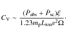
After applying this equation to both components of the WA, we find a volume filling factor of
Solving Eq. (2) for each of the WA components in Mrk 279 tells us that the high-ionisation phase can extend up to ![]() 20 pc from the central source, whereas the low-ionisation component can extend up to
20 pc from the central source, whereas the low-ionisation component can extend up to ![]() 260 pc. A lower limit to R
is harder to reliably estimate in these circumstances. A very mild
constraint can be obtained using dynamical arguments. If we assume that
the measured outflow velocities should be greater than or equal to the
escape velocity from the AGN we have
260 pc. A lower limit to R
is harder to reliably estimate in these circumstances. A very mild
constraint can be obtained using dynamical arguments. If we assume that
the measured outflow velocities should be greater than or equal to the
escape velocity from the AGN we have

where G is the constant of gravity, M the mass of the supermassive black hole, and R the distance of the WA from the black hole. The mass of the central black hole in Mrk 279 is
With these caveats in mind, both WA components in Mrk 279 seem to be located further away than the BLR, which is at
![]() days-light according to the relation given in Wandel (2002), and it is likely associated with the putative dusty torus. Using the approximate relation of Krolik & Kriss (2001) for the inner edge of the torus
days-light according to the relation given in Wandel (2002), and it is likely associated with the putative dusty torus. Using the approximate relation of Krolik & Kriss (2001) for the inner edge of the torus
![]() in pc, where L44 is the 1-1000 Rydberg luminosity in units of 1044 erg s-1, we obtain
in pc, where L44 is the 1-1000 Rydberg luminosity in units of 1044 erg s-1, we obtain
![]() pc. In Fig. 9
we plot these estimates relative to the torus distance and the BLR.
Similar results were found for the compilation of 23 AGN of B05, where
it can be seen that the minimum and maximum WA distances for the
Seyferts and NLSy1s are consistently further out than the BLR and tend
to cluster around the location of the torus. This would rule out an
accretion disc wind origin for these absorbers and would be closer to
the torus wind origin proposed by Krolik & Kriss (2001).
pc. In Fig. 9
we plot these estimates relative to the torus distance and the BLR.
Similar results were found for the compilation of 23 AGN of B05, where
it can be seen that the minimum and maximum WA distances for the
Seyferts and NLSy1s are consistently further out than the BLR and tend
to cluster around the location of the torus. This would rule out an
accretion disc wind origin for these absorbers and would be closer to
the torus wind origin proposed by Krolik & Kriss (2001).
![\begin{figure}
\par\includegraphics[angle=-90,width=9cm,clip]{14091fg9.ps}
\end{figure}](/articles/aa/full_html/2010/12/aa14091-10/img140.png)
|
Figure 9:
Estimated minimum and maximum distances of both WA phases in Mrk 279 from the central engine in units of the torus distance
|
| Open with DEXTER | |
4.4 Energetics of the warm absorber
It would be interesting to know whether the outflows commonly associated to the WA have an impact on the interestellar medium of the host galaxy of the AGN or even further out in the intergalactic medium. We can estimate how much mass is carried out of the innermost parts of the AGN by means of the outflows and how it compares with the accreted matter onto the central supermassive black hole.
From Eq. (4) we find
![]()
![]() yr-1 and
yr-1 and
![]()
![]() yr-1, for the low- and high-
yr-1, for the low- and high-![]() components,
respectively. These values are consistent with those of the WA in other
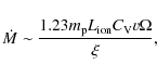
Seyfert 1 galaxies (see Blustin et al. 2005, and references therein). The mass accretion rate in Mrk 279 is calculated using
components,
respectively. These values are consistent with those of the WA in other
Seyfert 1 galaxies (see Blustin et al. 2005, and references therein). The mass accretion rate in Mrk 279 is calculated using

where we assume a nominal accretion efficiency of
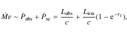
From the outflow rate we can estimate the importance of these
outflows in energetic terms. The kinetic luminosity (kinetic energy
carried out by the outflow per unit time) is defined as

With the
Given these
![]() values, the kinetic energy injected into the medium would be
values, the kinetic energy injected into the medium would be
![]() erg, assuming that the average AGN lifetime is of the order of
erg, assuming that the average AGN lifetime is of the order of
![]() years (Ebrero et al. 2009; Gilli et al. 2009). For instance, the energy needed to disrupt the ISM of a typical galaxy is estimated to be
years (Ebrero et al. 2009; Gilli et al. 2009). For instance, the energy needed to disrupt the ISM of a typical galaxy is estimated to be ![]() 1057 erg (Krongold et al. 2010), which means that the outflows in Mrk 279 are not powerful enough to critically affect the ISM of the host galaxy.
1057 erg (Krongold et al. 2010), which means that the outflows in Mrk 279 are not powerful enough to critically affect the ISM of the host galaxy.
4.5 Abundances in the warm absorber
We calculated the abundances of various elements in the WA of Mrk 279. The computed values were provided by xabs in SPEX and were calculated relative to a default set of standard abundances. In this work we have used the recent compilation of proto-solar abundances by Lodders (2003). Our results are reported in Table 6. We find the element abundances to be consistent with the solar ones in the cases of nitrogen and iron, carbon, and oxygen.
Arav et al. (2007) calculated the C, N, and O abundances in the WA of Mrk 279 using deep and simultaneous observations of Mrk 279 by FUSE and HST-STIS. The calculations of Arav et al. (2007) were done using CLOUDY v96b5 and the standard set of abundances was the default of that version of CLOUDY (Allende Prieto et al. 2001, for oxygen; Allende Prieto et al. 2002, for carbon; and Holweger 2001, for nitrogen). The differences between this set of standard abundances and that of Lodders (2003) is below 1%; therefore, we can compare our abundance determinations using Lodders with the results of Arav et al. (2007), finding that our results are fully consistent with theirs within the error bars with the exception of the nitrogen abundance, which was found to be slightly supersolar in Arav et al. (2007). On the other hand, we cannot confirm the significant supersolar abundances reported by Fields et al. (2007) using Chandra observations of Mrk 279.
Table 6: Abundances in the warm absorber of Mrk 279.
4.6 The lower ionisation emission lines
In the RGS spectrum, only the O VII narrow
forbidden line at 22.10 Å is detected. For other important
He-like and H-like ions we only obtain upper limits (see Table 5). We find that emission from the WA gas can easily reproduce the O VII
line and, at the same time, be consistent with the upper limits on the
other X-ray lines, provided that the covering factor of the gas is ![]() 0.1 (see Sect. 3.4).
This result is expected in type 1 objects, where the continuum
dominates the emission, as the absorption features of the ionised gas
along our line of sight are always more evident than the emission
lines. For instance, the O VII forbidden line does not display any outflow velocity but, as the measured blueshift for the absorption line is only
0.1 (see Sect. 3.4).
This result is expected in type 1 objects, where the continuum
dominates the emission, as the absorption features of the ionised gas
along our line of sight are always more evident than the emission
lines. For instance, the O VII forbidden line does not display any outflow velocity but, as the measured blueshift for the absorption line is only ![]() 370 km s-1, this would not be evident in the emission component, which is directed in a wider angle.
370 km s-1, this would not be evident in the emission component, which is directed in a wider angle.
Alternatively, O VII might come from reflection from the distant torus itself. To test this hypothesis, we used the model by Ross & Fabian (2005)
where reflection by constant-density and optically-thick material is
considered. The calculation includes a number of ions, in addition to
iron (REFLION model in XSPEC, Arnaud 1996). In particular, we used a modified version of REFLION where values lower than ![]() can be used (G. Miniutti, private communication) to reproduce high O VII to O VIII ratios. Indeed gas with
can be used (G. Miniutti, private communication) to reproduce high O VII to O VIII ratios. Indeed gas with ![]() (
(
![]() )
already produces a considerable amount of O VIII,
which is not representative of our data. The model, however, cannot be
tested directly on the RGS data, as the intrinsic resolution of the
model grid is only 0.3 Å, which is not appropiate for
high-resolution (
)
already produces a considerable amount of O VIII,
which is not representative of our data. The model, however, cannot be
tested directly on the RGS data, as the intrinsic resolution of the
model grid is only 0.3 Å, which is not appropiate for
high-resolution (
![]() )
data. We then fitted the EPIC-pn spectrum of Mrk 279 using XSPEC
and found the best-fit parameters for the reflection component. We went
on to evaluate the intrinsic line luminosities of O VII and O VIII
and compare them with the real measurements. Although the iron line at
6.4 keV can be fitted by the reflection model, the predicted soft
energy lines are not fully explained. We found that, within the allowed
range of best-fit
)
data. We then fitted the EPIC-pn spectrum of Mrk 279 using XSPEC
and found the best-fit parameters for the reflection component. We went
on to evaluate the intrinsic line luminosities of O VII and O VIII
and compare them with the real measurements. Although the iron line at
6.4 keV can be fitted by the reflection model, the predicted soft
energy lines are not fully explained. We found that, within the allowed
range of best-fit ![]() values (
values (![]() ),
the soft energy line luminosities are always overpredicted by the
model, by even a factor of 10 or more. This underlines the importance
of O VII and O VIII as diagnostic lines for cold reflection modelling.
),
the soft energy line luminosities are always overpredicted by the
model, by even a factor of 10 or more. This underlines the importance
of O VII and O VIII as diagnostic lines for cold reflection modelling.
5 Conclusions
We have analysed the absorption features present in the XMM-Newton-RGS
spectrum of Mrk 279, which are consistent with the existence of a warm
absorber at the redshift of the source. The absorbing material shows
two phases with different degrees of ionisation,
![]() and
and
![]() ,
and very shallow column densities (
,
and very shallow column densities (
![]() cm-2 and
cm-2 and
![]() cm-2, respectively).
cm-2, respectively).
The source was observed by XMM-Newton on three consecutive orbits during which it experienced a significant drop in brightness (up to a 20%) followed by a recovery. The WA did not show any significant variations in its parameters in response to the changes in flux. Likewise, no hints of significant long-term variability were found in Mrk 279 when comparing the current XMM-Newton and past Chandra observations. The best-fit parameters of the WA in both observations were found to be consistent within the error bars and a K-S test of the distribution of ionic column densities of C, O, Ne, and Fe between both observations only provided significancies lower than the 90% confidence level.
Following the argumentation of Blustin et al. (2005),
we were able to put mild constraints on the possible location of the
WA, finding that both components are likely located between a few pc
and up to ![]() 20 and
20 and ![]() 260 pc
for the high- and low-ionisation phases, respectively. This would mean
that the WA in Mrk 279 is likely to be associated to the putative dusty
torus rather than to the BLR or winds arising from the accretion disc.
The energetics of the WA outflows show that they have little or no
impact on the sourrounding ISM of the Mrk 279 host galaxy. Abundances
in the WA outflow were found to be consistent with Solar. The O VII
narrow forbidden line can be formed in the same gas that causes
absorption at soft energies, provided that the covering factor of the
gas, defined as the fraction of
260 pc
for the high- and low-ionisation phases, respectively. This would mean
that the WA in Mrk 279 is likely to be associated to the putative dusty
torus rather than to the BLR or winds arising from the accretion disc.
The energetics of the WA outflows show that they have little or no
impact on the sourrounding ISM of the Mrk 279 host galaxy. Abundances
in the WA outflow were found to be consistent with Solar. The O VII
narrow forbidden line can be formed in the same gas that causes
absorption at soft energies, provided that the covering factor of the
gas, defined as the fraction of ![]() sr
covered by the absorber as seen from the central source, is about 0.1.
This line is inconsistent with production by reflection in the
molecular torus.
sr
covered by the absorber as seen from the central source, is about 0.1.
This line is inconsistent with production by reflection in the
molecular torus.
The Space Research Organisation of The Netherlands is supported financially by NWO, The Netherlands Organisation for Scientific Research. We thank the anonymous referee for comments that improved this paper.
References
- Allende Prieto, C., Lambert, D. L., & Asplund, M. 2001, ApJ, 556, L63 [NASA ADS] [CrossRef] [Google Scholar]
- Allende Prieto, C., Lambert, D. L., & Asplund, M. 2002, ApJ, 573, L137 [NASA ADS] [CrossRef] [Google Scholar]
- Arav, N., Gabel, J. R., Korista, K. T., et al. 2007, ApJ, 658, 829 [NASA ADS] [CrossRef] [Google Scholar]
- Arnaud, K. A. 1996, Astronomical Data Analysis Software and Systems V, 101, 17 [NASA ADS] [Google Scholar]
- Baldwin, J., Ferland, G., Korista, K., & Verner, D. 1995, ApJ, 455, L119 [NASA ADS] [CrossRef] [Google Scholar]
- Behar, E. 2009, ApJ, 703, 1346 [NASA ADS] [CrossRef] [Google Scholar]
- Bianchi, S., Matt, G., Nicastro, F., et al. 2005, MNRAS, 357, 599 [NASA ADS] [CrossRef] [Google Scholar]
- Blustin, A. J., Page, M. J., Fuerst, S. V., et al. 2005, A&A, 431, 111 (B05) [NASA ADS] [CrossRef] [EDP Sciences] [Google Scholar]
- Cash, W. 1979, ApJ, 228, 939 [NASA ADS] [CrossRef] [Google Scholar]
- Crenshaw, D. M., Kraemer, S. B., Boggess, A., et al. 1999, ApJ, 516, 750 [NASA ADS] [CrossRef] [Google Scholar]
- Crenshaw, D. M., Kraemer, S. B., & George, I. M. 2003, ARA&A, 41, 117 [NASA ADS] [CrossRef] [Google Scholar]
- Costantini, E., Kaastra, J. S., Arav, N., et al. 2007, A&A, 461, 121 [NASA ADS] [CrossRef] [EDP Sciences] [Google Scholar]
- Costantini, E., Kaastra, J. S., Korista, K., et al. 2010, A&A, 512, 25 (Paper I) [Google Scholar]
- Dasyra, K. M., Ho, L. C., Armus, L., et al. 2008, ApJ, 674, 9 [NASA ADS] [CrossRef] [Google Scholar]
- Ebrero, J., Mateos, S., Stewart, G. C., et al. 2009, A&A, 500, 749 [NASA ADS] [CrossRef] [EDP Sciences] [Google Scholar]
- Elvis, M. 2000, ApJ, 545, 63 [NASA ADS] [CrossRef] [Google Scholar]
- Elvis, M., Wilkes, B. J., & Lockman, F. J. 1989, AJ, 97, 777 [NASA ADS] [CrossRef] [Google Scholar]
- Ferland, G. J., Korista, K. T., Verner, D. A., et al. 1998, PASP, 110, 761 [Google Scholar]
- Fields, D. L., Mathur, S., Krongold, Y., et al. 2007, ApJ, 666, 828 [NASA ADS] [CrossRef] [Google Scholar]
- Gabel, J. R., Arav, N., Kaastra, J. S., et al. 2005, ApJ, 623, 85 [Google Scholar]
- Gabriel, C., Denby, M., Fyfe, D. J., et al. 2004, in ADASS XIII, ed. F. Ochsenbein, M. Allen, & D. Egret, ASP Conf. Ser., 314, 759 [Google Scholar]
- George, I. M., Turner, T. J., Mushotzky, R. F., Nandra, K., & Netzer, H. 1998, ApJ, 503, 174 [NASA ADS] [CrossRef] [Google Scholar]
- Gibson, R. R., Canizares, C. R., Marshall, H. L., et al. 2007, ApJ, 655, 749 [NASA ADS] [CrossRef] [Google Scholar]
- Gilli, R., Zamorani, G., Miyaji, T., et al. 2009, A&A, 494, 33 [NASA ADS] [CrossRef] [EDP Sciences] [Google Scholar]
- Holweger, H. 2001, AIP Conf. Proc., 598, 23 [Google Scholar]
- Kaastra, J. S., & Barr, P. 1989, A&A, 226, 59 [NASA ADS] [Google Scholar]
- Kaastra, J. S., Mewe, R., & Nieuwenhuijzen, H. 1996, 11th Colloquium on UV and X-ray Spectroscopy of Astrophysical and Laboratory Plasmas, 411 [Google Scholar]
- Kaastra, J. S., Mewe, R., Liedahl, D. A., et al. 2000, A&A, 354, 83 [Google Scholar]
- Kaastra, J. S., Steenbrugge, K. C., Raassen, A. J. J., et al. 2002, A&A, 386, 427 [NASA ADS] [CrossRef] [EDP Sciences] [Google Scholar]
- Kaspi, S., Brandt, W. N, Netzer, H., et al., 2001, ApJ, 554, 216 [NASA ADS] [CrossRef] [Google Scholar]
- Kinkhabwala, A., Sako, M., Behar, E., et al. 2002, 575, 732 [Google Scholar]
- Krolik, J. H., & Kriss, G. A. 2001, ApJ, 561, 684 [NASA ADS] [CrossRef] [Google Scholar]
- Krongold, Y., Nicastro, F., Brickhouse, N. S., et al. 2003, ApJ, 597, 832 [NASA ADS] [CrossRef] [Google Scholar]
- Krongold, Y., Nicastro, F., Brickhouse, N. S., et al. 2005, ApJ, 622, 842 [NASA ADS] [CrossRef] [Google Scholar]
- Krongold, Y., Nicastro, F., Elvis, M., et al., 2007, ApJ, 659, 1022 [NASA ADS] [CrossRef] [Google Scholar]
- Krongold, Y., Elvis, M., Andrade-Velázquez, M., et al., 2010, ApJ, 710, 360 [NASA ADS] [CrossRef] [Google Scholar]
- Lodders, K. 2003, ApJ, 591, 1220 [NASA ADS] [CrossRef] [Google Scholar]
- Maiolino, R., & Riecke, G. H. 1995, ApJ, 454, 95 [NASA ADS] [CrossRef] [Google Scholar]
- Miller, L., Turner, T. J., & Reeves, J. N. 2008, A&A, 483, 437 [NASA ADS] [CrossRef] [EDP Sciences] [Google Scholar]
- Murray, N., & chiang, J. 1995, ApJ, 454, 105 [Google Scholar]
- Netzer, H. 1993, ApJ, 411, 594 [NASA ADS] [CrossRef] [Google Scholar]
- Netzer, H. 1996, ApJ, 473, 781 [NASA ADS] [CrossRef] [Google Scholar]
- Netzer, H., Chelouche, D., George, I. M., et al. 2002, ApJ, 571, 264 [Google Scholar]
- Netzer, H., Kaspi, S., Behar, E., et al. 2003, ApJ, 599, 933 [NASA ADS] [CrossRef] [Google Scholar]
- Nicastro, F., Fiore, F., & Matt, G. 1999, ApJ, 517, 108 [NASA ADS] [CrossRef] [Google Scholar]
- Nicastro, F., Zezas, A., Drake, J., et al. 2002, ApJ, 573, 157 [NASA ADS] [CrossRef] [Google Scholar]
- Ogle, P. M., Mason, K. O., Page, M. J., et al. 2004, ApJ, 606, 151 [NASA ADS] [CrossRef] [Google Scholar]
- Rees, M. J. 1984, ARA&A, 22, 471 [NASA ADS] [CrossRef] [Google Scholar]
- Reynolds, C. S. 1997, MNRAS, 286, 513 [NASA ADS] [CrossRef] [Google Scholar]
- Risaliti, G., Miniutti, G., Elvis, M., et al. 2009, ApJ, 696, 160 [NASA ADS] [CrossRef] [Google Scholar]
- Ross, R. R., & Fabian, A. C. 2005, MNRAS, 358, 211 [Google Scholar]
- Scott, J. E., Kriss, G. A., Lee, J. C., et al., 2004, ApJS, 152, 1 [NASA ADS] [CrossRef] [Google Scholar]
- Spergel, D. N., Verde, L., Peiris, H. V., et al. 2003, ApJS, 148, 175 [NASA ADS] [CrossRef] [Google Scholar]
- Steenbrugge, K. C., Kaastra, J. S., Crenshaw, D. M., et al. 2005, A&A, 434, 569 [NASA ADS] [CrossRef] [EDP Sciences] [Google Scholar]
- Wandel, A. 2002, ApJ, 565, 762 [NASA ADS] [CrossRef] [Google Scholar]
- Weaver, K. A., Arnaud, K. A., & Mushotzky, R. F. 1995, ApJ, 447, 121 [NASA ADS] [CrossRef] [Google Scholar]
- Weaver, K. A., Gelbord, J., & Yaqoob, T. 2001, ApJ, 560, 261 [NASA ADS] [CrossRef] [Google Scholar]
- Williams, R. J., Mathur, S., & Nicastro, F. 2006, ApJ, 645, 179 [NASA ADS] [CrossRef] [Google Scholar]
Footnotes
- ... SPEX
![[*]](/icons/foot_motif.png)
- http://www.sron.nl/spex/
- ... obtained
- In Eq. (23) in Blustin et al. (2005,) there was a typo in the denominator of the equation: c should not be there.
All Tables
Table 1: XMM- Newton observation log.
Table 2: Mrk 279 RGS continuum best-fit parameters.
Table 3: Best-fit xabs parameters to the warm absorber of Mrk 279.
Table 4: Column densitity and outflow velocity of the most relevant X-ray absorption lines.
Table 5: Emission line luminosities measured by RGS and their significance.
Table 6: Abundances in the warm absorber of Mrk 279.
All Figures
|
|
Figure 1: EPIC-pn lightcurve in the 0.3-2 keV band. |
| Open with DEXTER | |
| In the text | |
|
|
Figure 2: Average spectral energy distribution of Mrk 279. The X-ray continuum is determined by Chandra (crosses, Costantini et al. 2007). For comparison, we overplot the average continuum measured by XMM- Newton (diamonds). For the far UV we relied on the HST and FUSE measurements. |
| Open with DEXTER | |
| In the text | |
|
|
Figure 3: RGS spectrum of Mrk 279. For plotting purposes all three observations have been stacked into a single spectrum. The solid line corresponds to the best-fit model. The most relevant spectral features are labelled. |
| Open with DEXTER | |
| In the text | |
|
|
Figure 4: Detail of the O VIII absorption line. Overplotted is the fit with only one xabs component (dashed line) and two xabs components (solid line). |
| Open with DEXTER | |
| In the text | |
|
|
Figure 5: Comparison between the H (black crosses) and L (light stars) datasets. The L dataset is normalised to the unabsorbed continuum of the H dataset. |
| Open with DEXTER | |
| In the text | |
|
|
Figure 6:
Emission line contribution of the warm absorbers in Mrk 279, assuming a covering fraction
|
| Open with DEXTER | |
| In the text | |
|
|
Figure 7: Pressure ionisation parameter as a function of electron temperature. The values corresponding to the warm absorber components in Mrk 279 are marked as squares. |
| Open with DEXTER | |
| In the text | |
|
|
Figure 8:
Ionic column densities of Fe (upper left panel), Ne (upper right panel), C (lower left panel), and O (lower right panel) ions in the XMM- Newton (solid lines, this work; dots: low- |
| Open with DEXTER | |
| In the text | |
|
|
Figure 9:
Estimated minimum and maximum distances of both WA phases in Mrk 279 from the central engine in units of the torus distance
|
| Open with DEXTER | |
| In the text | |
Copyright ESO 2010
Current usage metrics show cumulative count of Article Views (full-text article views including HTML views, PDF and ePub downloads, according to the available data) and Abstracts Views on Vision4Press platform.
Data correspond to usage on the plateform after 2015. The current usage metrics is available 48-96 hours after online publication and is updated daily on week days.
Initial download of the metrics may take a while.