| Issue |
A&A
Volume 520, September-October 2010
|
|
|---|---|---|
| Article Number | A35 | |
| Number of page(s) | 11 | |
| Section | Galactic structure, stellar clusters, and populations | |
| DOI | https://doi.org/10.1051/0004-6361/200913933 | |
| Published online | 27 September 2010 | |
Chemical evolution models for spiral disks: the Milky Way, M 31, and M 33
M. M. Marcon-Uchida1,2 - F. Matteucci1,3 - R. D. D. Costa2
1 - Dipartimento di Fisica, Sezione di Astronomia, Università di Trieste, via GB Tiepolo 11, 34131 Trieste, Italy
2
- Instituto de Astronomia, Geofísica e Ciências Atmosféricas (IAG),
Universidade de São Paulo, Rua do Matão, 1226 Cidade Universitária, São
Paulo - SP 05508-900, Brazil
3 -
INAF Osservatorio Astronomico di Trieste, via GB Tiepolo 11, 34131 Trieste, Italy
Received 21 December 2010 / Accepted 22 April 2010
Abstract
Context. The distribution of chemical abundances and their
variation with time are important tools for understanding the chemical
evolution of galaxies. In particular, the study of chemical evolution
models can improve our understanding of the basic assumptions made when
modelling our Galaxy and other spirals.
Aims. We test a standard chemical evolution model for spiral
disks in the Local Universe and study the influence of a threshold gas
density and different efficiencies in the star formation rate (SFR) law
on radial gradients of abundance, gas, and SFR. The model is then
applied to specific galaxies.
Methods. We adopt a one-infall chemical evolution model where
the Galactic disk forms inside-out by means of infall of gas, and we
test different thresholds and efficiencies in the SFR. The model is
scaled to the disk properties of three Local Group galaxies (the Milky
Way, M 31 and M 33) by varying its dependence on the star
formation efficiency and the timescale for the infall of gas onto the
disk.
Results. Using this simple model, we are able to reproduce most
of the observed constraints available in the literature for the studied
galaxies. The radial oxygen abundance gradients and their time
evolution are studied in detail. The present day abundance gradients
are more sensitive to the threshold than to other parameters, while
their temporal evolutions are more dependent on the chosen SFR
efficiency. A variable efficiency along the galaxy radius can reproduce
the present day gas distribution in the disk of spirals with prominent
arms. The steepness in the distribution of stellar surface density
differs from massive to lower mass disks, owing to the different star
formation histories.
Conclusions. The most massive disks seem to have evolved faster
(i.e., with more efficient star formation) than the less massive ones,
thus suggesting a downsizing in star formation for spirals. The
threshold and the efficiency of star formation play a very important
role in the chemical evolution of spiral disks. For instance, an
efficiency varying with radius can be used to regulate the star
formation. The oxygen abundance gradient can steepen or flatten in time
depending on the choice of this parameter.
Key words: galaxies: abundances - galaxies: evolution - galaxies: spiral
1 Introduction
The study of the chemical evolution of nearby spiral galaxies is very important to improving our knowledge of the main ingredients used in chemical evolution models and testing the basic assumptions made in modelling our Galaxy. The other spiral members of the Local Group of galaxies M 31 and M 33 have been the target of many observational studies to investigate the chemical and dynamical properties of these neighbouring systems. New surveys (Braun et al. 2009; Magrini et al. 2007 2008) have contributed to the analysis of different stellar populations and provided more accurate data to constrain the chemical evolution models.
The disks of M 31 and M 33 have many similarities with the Milky Way disk but some observational constraints such as the present day gas distribution can only be explained by assuming different star formation histories for these galaxies. The SFR is one of the most important parameters regulating the chemical evolution of galaxies (Kennicutt 1998; Matteucci 2001; Boissier et al. 2003) together with the initial mass function (IMF).
The ``inside-out'' formation of the disk is an important mechanism for reproducing the radial abundance gradients (see Colavitti et al. 2008, for the most recent paper on the subject). A more rapid formation of the inner disk relative to the outer disk was originally proposed by Matteucci & François (1989) and supported in the following years by Boissier & Prantzos (1999) and Chiappini et al. (2001).
The chemical evolution of M 31 has already been compared with that of the Milky Way by Renda et al. (2005) and Yin et al. (2009). Renda et al. (2005) concluded that while the evolution of the MW and M 31 share similar properties, differences in the formation history of these two galaxies are required to explain the observations in detail. In particular, they found that the observed higher metallicity of the M 31 halo can be explained by either (i) a higher halo star formation efficiency; or (ii) a larger reservoir of infalling halo gas with a longer halo formation phase. These two different scenarios would lead to either (i) a higher [O/Fe] at low metallicities, or (ii) younger stellar populations in the M 31 halo, respectively. Both scenarios produce a more massive stellar halo in M 31, which suggests that there is a correlation between the halo metallicity and its stellar mass. Yin et al. (2009) concluded that M 31 must have been more active in the past than the Milky Way, despite its current SFR being lower than that of the Milky Way, and that our Galaxy must be a rather quiescent galaxy, atypical of its class (see also Hammer et al. 2007). They also concluded that the star formation efficiency in M 31 must have been higher by a factor of two than in the Galaxy. However, by adopting the same SFR as in the Milky Way they failed to reproduce the observed radial profile of both the star formation and of the gas, and suggested that possible dynamical interactions could explain these distributions.
Regarding M 33, some works (e.g. Magrini et al. 2007) computed the chemical evolution of its disk reproducing the observational features by assuming a continuous almost constant infall of gas. In addition, the authors also concluded that the metallicity of M 33's disk had increased with time and that the radial abundance gradient has a tendency to flatten during the galaxy evolution.
In this work, we present a one-infall chemical evolution model for the Galactic disk based on an updated version of the Chiappini et al. (2001) model. This model can predict the evolution of the abundances of 37 chemical elements from the light to the heavy ones. We use this model to reproduce the chemical evolution of the Milky Way disk and that of the two nearby spiral galaxies (M 31 and M 33). To do that, we assume that the disk of each galaxy formed by gas accretion and vary the star formation efficiency as well as the gas accretion timescale. The similarities and the differences between the chemical evolution of these objects and the Milky Way are discussed to provide a basis for the understanding of the chemical evolution of disks.
The paper is organized as follows. In Sect. 2, we describe our chemical evolution model and the assumptions made for each galaxy. In Sect. 3, we present the results for the models and discuss these in detail in Sect. 4. Finally in Sect. 5 we summarize our conclusions.
2 The chemical evolution model
To reproduce the chemical evolution of the thin-disk, we adopted an updated one-infall version of the chemical evolution model presented by Chiappini et al. (2001, hereafter CMR2001). In this model, the galactic disk is divided into several concentric rings that evolve independently without exchange of matter.
The disk is built up in the context of an ``inside-out'' scenario,
which is necessary to reproduce the radial abundance gradients
(Colavitti et al. 2008). The infall law for the thin disk is defined as
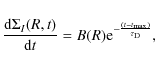
where
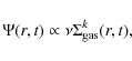
To make the program as simple and generalized as possible, we used a SFR proportional to a Schmidt law
|
(2) |
where
Table 1: Coefficients for the timescale equation.
According to recent studies (e.g. Romano et al. 2005),
the IMF and the stellar lifetimes are primarily responsible for
uncertanties in the chemical evolution models of the Milky Way. In this
work, we assumed that the IMF is constant in space and time and adopted
the prescription from Kroupa (1993), instead of the two-slope approximation of Scalo (1986) used by CMR2001.
The total surface mass density distribution for the Galactic disk was assumed to be exponential with scale length
![]() kpc normalized to
kpc normalized to
![]() pc-2 (Romano et al. 2000)
pc-2 (Romano et al. 2000)
|
(3) |
Apart from the IMF, this model differs from that of the CMR2001 model in terms of: (1) the oxygen yields for massive stars that are supposed to be metallicity-dependent and taken from Woosley & Weaver (1995), as suggested in François et al. (2004); (2) the stellar lifetimes of Schaller et al. (1992) instead of the Maeder & Meynet (1989); and (3) the solar abundances are those from Asplund et al. (2009).
2.1 The Milky Way
We computed the model for the Milky Way several times with star formation efficiency of 1 Gyr-1 and different timescales for the gas infall onto the disk (![]() ). Table 1 shows the coefficients for the linear equations adopted for
). Table 1 shows the coefficients for the linear equations adopted for ![]() .
Figure 1 illustrates the predictions for the dwarf metallicity distribution in the solar neighbourhood (Scalo 1986, represented as a dotted line and Kroupa et al. 1993,
represented as a dashed line) and the observed corrected values from
the Geneva-Copenhagen Survey (GCS) as presented in Holmberg et al.
(2007). The model predictions using the IMF of Kroupa (1993)
provide a closer fit to the wings of the dwarf distribution, especially
for higher metallicities and produce fewer metal-poor stars, reducing
the well-known ``G-dwarf'' problem.
.
Figure 1 illustrates the predictions for the dwarf metallicity distribution in the solar neighbourhood (Scalo 1986, represented as a dotted line and Kroupa et al. 1993,
represented as a dashed line) and the observed corrected values from
the Geneva-Copenhagen Survey (GCS) as presented in Holmberg et al.
(2007). The model predictions using the IMF of Kroupa (1993)
provide a closer fit to the wings of the dwarf distribution, especially
for higher metallicities and produce fewer metal-poor stars, reducing
the well-known ``G-dwarf'' problem.
![\begin{figure}
\par\includegraphics[width=9cm,clip]{13933fg1.eps}
\end{figure}](/articles/aa/full_html/2010/12/aa13933-09/img16.png)
|
Figure 1:
Distribution of dwarf stars in the solar vicinity obtained by using different IMFs. Scalo (1986, dotted line) and Kroupa et al. (1993, dashed line) compared to the
observational data of Holmberg et al. (2007, solid line). The label ``New tau'' indicates that we have used the |
| Open with DEXTER | |
![\begin{figure}
\par\includegraphics[width=9cm,clip]{13933fg2.eps}
\end{figure}](/articles/aa/full_html/2010/12/aa13933-09/img17.png)
|
Figure 2: Different time scales for infalling gas along the disk tested in this work. Solid line for this work, dashed line for CMR2001, dotted line for Carigi et al. (2008), dot-dashed for Boissier & Prantzos (1999), filled circles for Renda et al. (2005), and dot-dot-dashed lines for Chang et al. (1999). |
| Open with DEXTER | |
In Fig. 2, we show the
different gas infall laws tested in this work and taken from the
literature; the vertical line marks the radius corresponding to the
solar vicinity at 8 kpc. Comparing the results of the dwarf
metallicity distributions (Fig. 3) obtained with the different ![]() ,
we note that the timescale for the infalling gas affects the total
number of dwarf stars produced by each model. The law presented by
Renda et al. (2005)
reproduces more closely the fraction of stars observed in the GCS of
the solar neighbourhood, but the timescale for the solar radius that
they adopted (see Fig. 2),
around 12 Gyr, is unrealistic. In this work, the timescale for the
infalling gas, was derived based on the distribution of dwarf stars in
the solar neighbourhood, from which we know that it should be
about 7 to 8 Gyr assuming that the outermost regions of the
Galaxy are still forming now. This particular form of the
,
we note that the timescale for the infalling gas affects the total
number of dwarf stars produced by each model. The law presented by
Renda et al. (2005)
reproduces more closely the fraction of stars observed in the GCS of
the solar neighbourhood, but the timescale for the solar radius that
they adopted (see Fig. 2),
around 12 Gyr, is unrealistic. In this work, the timescale for the
infalling gas, was derived based on the distribution of dwarf stars in
the solar neighbourhood, from which we know that it should be
about 7 to 8 Gyr assuming that the outermost regions of the
Galaxy are still forming now. This particular form of the ![]() also can fit the abundance, gas and SFR gradients, as we will show in the following sections.
also can fit the abundance, gas and SFR gradients, as we will show in the following sections.
On the other hand, the position of the peak and its wings are more important constraints, since owing to observational difficulties we have problems defining the completeness of the survey (Holmberg et al. 2007). Focusing on these quantities, one can note that time scales given by CMR2001 and this work closely reproduce the position of the peak in the observed distribution as well as the high metallicity wing, whereas at the low metallicity side the number of stars is slightly overestimated, although this effect disappears if we consider other distributions (Fig. 3, right panel). Schönrich & Binney (2009) also reproduced the [Fe/H] distribution in the solar neighbourhood by means of a chemo-dynamical model suggesting that the G-dwarf distribution can be explained well by stellar migration, without considering inside-out formation. However, the churning and blurring mechanisms invoked there imply a gas transfer that results in a similar effect.
![\begin{figure}
\par\includegraphics[width=17cm]{13933fg3.eps}
\end{figure}](/articles/aa/full_html/2010/12/aa13933-09/img18.png)
|
Figure 3:
Predicted dwarf stellar metallicity distributions for the Milky Way. Left panel shows different distributions estimated with the various |
| Open with DEXTER | |
After setting the ideal value for the time scale of the infalling gas (
![]() ),
a test was perfomed assuming a variable star formation efficiency along
the galactic disk. An efficiency that decreases with galactic radius
was adopted until it reached the lower limit of 0.5 Gyr-1
at 12 kpc. This value is similar to that adopted in successful
models of dwarf irregular and spheroidal galaxies (see Lanfranchi &
Matteucci 2003). To test our assumption of a variable
),
a test was perfomed assuming a variable star formation efficiency along
the galactic disk. An efficiency that decreases with galactic radius
was adopted until it reached the lower limit of 0.5 Gyr-1
at 12 kpc. This value is similar to that adopted in successful
models of dwarf irregular and spheroidal galaxies (see Lanfranchi &
Matteucci 2003). To test our assumption of a variable ![]() ,
we show in Fig. 4 a plot of the empirical
,
we show in Fig. 4 a plot of the empirical
![]() ,
obtained by adopting the observed SFR and
,
obtained by adopting the observed SFR and
![]() for the three galaxies. As one can see, for all the galaxies the
``observed efficiency'' shows a decreasing profile compatible with the
trend used in our models.
for the three galaxies. As one can see, for all the galaxies the
``observed efficiency'' shows a decreasing profile compatible with the
trend used in our models.
2.2 M 31
M 31 is a nearby spiral galaxy around two times more massive and 2.4 times larger than the Milky Way (Yin et al. 2009). It is of an earlier type than the Milky Way possessing a larger bulge.
To reproduce the chemical evolution of M 31, we adopted the same model used for the Milky Way with the following modifications:
- (i)
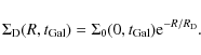
- Surface mass density distribution: assumed to be exponential with the scale-length radius
 kpc and central surface
density
kpc and central surface
density
 pc-2, as suggested by Geehan et al. (2006).
- (ii)
- Time scale for the infalling gas:
 .
This relation was based the assumption that at the galactocentric distance equivalent to the solar radius (the R corresponding to the
.
This relation was based the assumption that at the galactocentric distance equivalent to the solar radius (the R corresponding to the  calculated on the basis of the
 ratio), M 31 should have a timescale for the infall of gas similar
to that of the solar vicinity. In addition, the outermost part of the
optical disk continues to accrete gas.
ratio), M 31 should have a timescale for the infall of gas similar
to that of the solar vicinity. In addition, the outermost part of the
optical disk continues to accrete gas. - (iii)
- Star formation efficiency: the M 31 present-day
gas profile in the disk exhibits a different trend relative to the
Milky Way. It increases with galactic radius and, after reaching a peak
(at around 12 kpc) decreases steeply towards the center, thus
suggesting a different scenario, from that of the Milky Way, for the
star formation history of this galaxy. This trend is the signature of a
very prominent spiral arm detectable in M 31 thanks to its
relatively high inclination angle, which allows us to measure the
column density of the hydrogen distribution.
To reproduce the gas distribution we adopted three different star formation efficiencies. In model M 31-A1 we assumed Gyr-1 (same as the Milky Way), in model M 31-A2 it was set to be equal to 2 Gyr-1, whereas in model M 31-B it was assumed to be a function of the galaxy radius
 ,
until it reached a minimum value of 0.5 Gyr-1 and was then
assumed to be constant.
,
until it reached a minimum value of 0.5 Gyr-1 and was then
assumed to be constant.
- (iv)
- Threshold in the star formation: we adopted a threshold in gas density of 5
 /pc2, as suggested by Braun et al. (2009).
- (v)
- Exponent in the star formation law: for this galaxy, we also tested a model with a different exponent k in the Schmidt law, using the lower limit given by Kennicutt et al. (1998), k=1.25 (this model is indicated by M 31-Bk1.25).
2.3 M 33
M 33 or Triangulum Galaxy (NGC598) is a low-density late-type galaxy of the Local Group and exhibits no notable signatures of a bar or recent mergers. To model the chemical evolution of M 33 we adopted the following parameters:
- (i)
- Surface mass density distribution: assumed to be exponential with the scale-length radius
 kpc (Corbelli 2003) and central surface density
 pc-2.
pc-2.
- (ii)
- Time scale for the infalling gas: set in the same way as M 31, as explained in Sect. 2.2, with
 .
.
- (iii)
- Star formation efficiency: for this galaxy, we also used three different models. Two of them had constant efficiency equal to
 Gyr-1 and
  Gyr-1 and another one with a efficiency that decreases with the radius:
 ,
in this case we did not adopt a minimum value for the star formation
efficiency because of the low density profile of this galaxy.
,
in this case we did not adopt a minimum value for the star formation
efficiency because of the low density profile of this galaxy. - (iv)
- Threshold in the star formation:
 /pc2.
We adopted a lower value for the threshold because of its diverse
environmental conditions as a consequence of its lower mass.
/pc2.
We adopted a lower value for the threshold because of its diverse
environmental conditions as a consequence of its lower mass.
![\begin{figure}
\par\includegraphics[width=9cm,clip]{13933fg4a.eps}\par\includegr...
...{13933fg4b.eps}\par\includegraphics[width=9cm,clip]{13933fg4c.eps}
\end{figure}](/articles/aa/full_html/2010/12/aa13933-09/img38.png)
|
Figure 4: Estimate of the present-day star formation efficiency using the observed gas surface density and star formation rate. The first panel shows the values for the MW (we used two different gas distributions and the SFR of Rana 1991), second panel is for M 31 (using the gas distribution of Yin et al. 2009; and the SFR of Boissier et al. 2007), while the last one shows the M 33 values (using the gas distributions of Corbelli et al. 2003; and Boissier et al. 2007; and the SFR of Heyer et al. 2004; and Hoopes & Walterbros 2000). |
| Open with DEXTER | |
3 Results
To reproduce the observational chemical constraints of the spiral disks
of three Local Group galaxies (MW, M 31, and M 33) and to
study the common features in the evolution of these systems, we
computed several models by varying the three parameters shown in Table
2 (![]() ,
,
![]() and the threshold).
and the threshold).
Table 2: Models parameters.
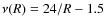
In the following sections, we compare our results for the radial
gradients of oxygen abundance, present-day gas and stellar density
distribution and SFR for all three galaxies. In each case a comparison
between the disks is made using the normalized radius
![]() .
In Figs. 5, 7, and 8, solid and dotted lines represent the models with constant star formation efficiency
.
In Figs. 5, 7, and 8, solid and dotted lines represent the models with constant star formation efficiency
![]() ,
namely MW-A1, MW-A2 M 31-A1, M 31-A2, M 33-A05, and
M 33-A01. Dashed lines represent the models in wich the efficiency
is a function of the galactic radius,
,
namely MW-A1, MW-A2 M 31-A1, M 31-A2, M 33-A05, and
M 33-A01. Dashed lines represent the models in wich the efficiency
is a function of the galactic radius, ![]() ,
models: MW-B, M 31-B, M 31-Bk1.25 (dot-dashed), and M 33-B (see Table 2
for details). In the bottom right panel of those figures, we present
the comparison between the variable star formation efficiency models
for each galaxy, where the solid line represents the Milky Way, while
dashed and dotted lines represent M 31 and M 33,
respectively.
,
models: MW-B, M 31-B, M 31-Bk1.25 (dot-dashed), and M 33-B (see Table 2
for details). In the bottom right panel of those figures, we present
the comparison between the variable star formation efficiency models
for each galaxy, where the solid line represents the Milky Way, while
dashed and dotted lines represent M 31 and M 33,
respectively.
Table 3: Current values for the oxygen abundance gradient from the models for the galaxies in study.
3.1 Oxygen abundance gradient
The effect of the variable efficiency in the SFR can also be noted in
our models. As expected, when comparing models with the same threshold
we can see that those for wich ![]() exhibit a steeper gradient than the models with constant efficiency.
exhibit a steeper gradient than the models with constant efficiency.
![\begin{figure}
\par\includegraphics[width=17cm]{13933fg5.eps}
\end{figure}](/articles/aa/full_html/2010/12/aa13933-09/img44.png)
|
Figure 5:
Radial oxygen abundance gradient for the three galaxies in the sample. Milky Way data: HII regions from Deharveng et al. (2000), Esteban et al. (2005), Rudolph et al. (2006), Cepheids from Andrievsky et al. (2002a,b), and planetary nebulae from Costa et al. (2004). The right upper panel shows HII regions observed in M 31, data from: Galarza et al. (1999), Trundle et al. (2002), Blair et al. (1982) and Dennefeld & Kunth (1981). For M 33 ( left lower panel),
the observed data are HII Regions from Rosolowsky et al. (2007)
and type I Planetary Nebulae from Magrini et al. (2009).
In these figures, solid lines are for MW-A1, M 31-A1 and
M 33-A05 and dotted lines represent the models MW-A2,
M 31-A2, and M 33-A01 while dashed lines show the results of
the models Mw-B, M 31-B (dot-dahed for M 31-Bk1.25), and
M 33-B (see Table 2 for details). The lower right panel shows the model prediction with variable |
| Open with DEXTER | |
In Fig. 5, we show the
results for the oxygen abundance gradient for the Milky Way (left upper
panel), M 31 (right upper panel), and M 33 (left lower panel)
with a compilation of observational data and a comparative plot between
the predictions for the galaxies (right lower panel). The abundance
results are slightly shifted for the MW and overestimated for
M 33, but the predicted slopes of the gradients are in agreement
with the observational data. The threshold effect can be interpreted in
terms of the breaks in the gradients being more significant for the MW
and M 33 than for M 31 (except when k=1.25) because M 31 has a more massive disk.
Table 3
shows the present-day values of the radial abundance gradient of the
oxygen in different galactocentric distance ranges as predicted by our
models, compared with the observed values for the three galaxies. The
predictions of all our models are in very good agreement with
observational data and the effect of different thresholds can be seen
in the results of the Milky Way models with constant efficiency in the
SFR. Model MW-A1 (threshold of
![]() pc-2) has much steeper gradients than the values predicted by MW-A2 (threshold equal to
pc-2) has much steeper gradients than the values predicted by MW-A2 (threshold equal to
![]() pc-2), which is a consequence of the suppression of the star formation.
pc-2), which is a consequence of the suppression of the star formation.
![\begin{figure}
\par\includegraphics[width=17cm]{13933fg6.eps}
\end{figure}](/articles/aa/full_html/2010/12/aa13933-09/img46.png)
|
Figure 6: Time evolution of the slope of the radial abundance gradient of oxygen for all models. The first panel shows the results for the Milky Way (solid line for Mw-A1, dotted line for MW-A2, and dashed line for MW-B), while the middle panel is for M 31 (solid line for M 31-A1, dotted line for M 31-A2, dashed line for M 31-B, and dot-dashed line for M 31-Bk1.25) and the last panel shows the predictions for M 33 (solid line for M 33-A05, dotted line for M 33-A01, and dashed line for M 33-B). See Table 2 for more details. |
| Open with DEXTER | |
![\begin{figure}
\par\includegraphics[width=17cm]{13933fg7.eps}
\end{figure}](/articles/aa/full_html/2010/12/aa13933-09/img47.png)
|
Figure 7:
Present-day radial gas distribution. Milky Way data: Rana (1991) and Dame et al. (1993). M 31: solid circles represents the total gas data from Braun et al. (2009) and crosses represents HI data from Chemin et al. (2009). M 33: data from Boissier et al. (2007) and Verley et al. (2008).
In these figures, solid lines are for MW-A1, M 31-A1, and
M 33-A05 and dotted lines represent the models MW-A2,
M 31-A2, and M 33-A01, while dashed lines show the results of
the models Mw-B, M 31-B, and M 33-B (see Table 2 for details). The lower right panel shows the model prediction with variable |
| Open with DEXTER | |
Figure 6 shows the evolution of the oxygen abundance gradient with time. Models are the same as those presented in Table 2.
It is not easy to establish wether the radial abundance gradient tends
to flatten or steepen with time: the models predict either flattening
or steepening of the gradient depending on the adopted SFR along the
disk. As one can see, for ![]() all models predict a gradient that flattens with time. Gradients that
flatten with time with a decreasing flattening rate in the past few
Gyrs are supported by models such as those proposed by Hou et al. (2000), Mollà & Diaz (2005), and Magrini et al. (2009), while models proposed by Tosi (1988) and CMD2001 predict a steepening of the gradients in time. Observational results by Maciel et al. (2003) support the flattening with time of the oxygen abundance gradient in the Milky Way, while Magrini et al. (2009) also noted a flattening of the oxygen gradient in their sample of M 33 planetary nebulae.
all models predict a gradient that flattens with time. Gradients that
flatten with time with a decreasing flattening rate in the past few
Gyrs are supported by models such as those proposed by Hou et al. (2000), Mollà & Diaz (2005), and Magrini et al. (2009), while models proposed by Tosi (1988) and CMD2001 predict a steepening of the gradients in time. Observational results by Maciel et al. (2003) support the flattening with time of the oxygen abundance gradient in the Milky Way, while Magrini et al. (2009) also noted a flattening of the oxygen gradient in their sample of M 33 planetary nebulae.
3.2 Gas and stellar surface-density distribution
Figure 7 shows the present-day gas surface-density distribution for the galaxies studied here. For the Milky Way, we note that the model MW-B describes the most closely the present gas surface density of the disk with a smoother distribution while MW-A1 and MW-A2 exhibit notable breaks in the profile (probably associated with the constant efficiency in the SFR).
For M 31, the models with constant star formation efficiencies can reproduce an exponential profile but fail to explain the peak located at about a distance of 12 kpc from the galaxy center. The models with variable efficiency (M 31-B and M 31-Bk1.25) can reproduce this peak as shown in Fig. 7. Both models for M 33 are capable of explaining the present day-gas distribution of Boissier et al. (2007) for R> 4 kpc, but overestimate the gas surface density in the inner regions.
In Fig. 9, we show the
predicted stellar density distributions along the three disks. The
Milky Way models are in good agreement with the observed values (shaded
area). All this area was obtained by assuming an exponential
distribution (see also CMR2001), and using a scale-length radius
![]() equal to 2.5 kpc (Freudenreich 1998), and a stellar density for the solar annulus equal to
equal to 2.5 kpc (Freudenreich 1998), and a stellar density for the solar annulus equal to
![]() pc-2
(Gilmore et al. 1998), to scale the distribution to the observed
values. The predictions for the stellar density profile of M 31
show a shallower distribution, whereas for M 33 our models predict
a steeper distribution (even without taking into account the inner part
of the M 33 disk,whose stellar density is also overestimated as a
consequence of the gas profile - see Fig. 7).
pc-2
(Gilmore et al. 1998), to scale the distribution to the observed
values. The predictions for the stellar density profile of M 31
show a shallower distribution, whereas for M 33 our models predict
a steeper distribution (even without taking into account the inner part
of the M 33 disk,whose stellar density is also overestimated as a
consequence of the gas profile - see Fig. 7).
3.3 SFR
In Fig. 8, we compare the predicted SFR distributions of the three disks compared to observational data. All the models can reproduce the observational trends and the differences between the different model predictions for each galaxy is very small. For the MW, the models differ from the data only in the outer regions where the threshold in the star formation, i.e., that of the model MW-A1 (with the highest threshold density value) exhibits a steeper profile. The predictions for M 31 are of a higher SF than the observed data, which could be related to the the limitations of the method used to estimate the SFR in M 31(both uncertainties in the adopted IMF and the assumed metallicity in the conversion factors from the UV to the star formation rate values). The models M 33-A05 and M 33-B predict similar values of the star formation rate, which are in very good agreement with the observational data (except for the innermost region).
![\begin{figure}
\par\includegraphics[width=17cm]{13933fg8.eps}
\end{figure}](/articles/aa/full_html/2010/12/aa13933-09/img50.png)
|
Figure 8:
Present-day radial distribution of the SFR. Observational data for the Milky Way are those from Rana et al. (1991), for M 31 open circles represents the data from
Braun et al. (2009), and for M 33 the observation data are from Hoopes & Walterbros (2000), Heyer et al. (2004), and Kennicutt (1989).
In these figures, solid lines are for MW-A1, M 31-A1, and
M 33-A05 and dotted lines represent the models MW-A2,
M 31-A2, and M 33-A01, while dashed lines show the results of
the models MW-B, M 31-B, M 31-Bk1.25 (dot-dashed), and
M 33-B (see Table 2 for details). The lower right panel shows the model prediction for a variable |
| Open with DEXTER | |
3.4 Deuterium abundances
Figure 10 shows the deuterium radial abundance gradient for the three galaxies studied in this work. Previous studies have already shown that the abundance of D/H in the disk of the MW should increase with radius (e.g., Prantzos 1996; Romano et al. 2006), but this is the first time that this gradient has been computed for external galaxies. One can note that the deuterium gradient exhibits the opposite behaviour to the oxygen distribution with galactic radius, reflecting that D is destroyed only during galactic evolution. We show this diagram just as a prediction, since there are no data for M 31 or M 33, and for the MW there are data only for the local ISM.
In particular, the measures of the local abundance of D has a large
spread, which is indicative of different values along different lines
of sight. The most plausible interpretation of this is that D can
condense onto carbon grains and PAH molecules, thus being removed from
the ISM (Linsky et al. 2006,
and references therein). Moreover, another problem is that the highest
D abundance measured locally is higher than expected by chemical
evolution models, thus implying an astration factor of
![]() (Savage et al. 2007), while our model, for example, predicts a factor of
(Savage et al. 2007), while our model, for example, predicts a factor of ![]() 1.5 (we assume a primordial
1.5 (we assume a primordial
![]() in number, as suggested by WMAP). Some additional information about the
primordial D/H abundance comes from the measurements in QSO absorbers,
which provide a lower limit to the primordial D/H abundance. These
systems, in fact, are found at high redshift z>2
and their metallicity is low, thus their D/H, which is only destroyed
during galactic evolution, is likely to be close to the primordial
value. Pettini et al. (2008), in particular, analysed several QSO absorbers, the most distant being at z=2.61843 and having an oxygen abundance
in number, as suggested by WMAP). Some additional information about the
primordial D/H abundance comes from the measurements in QSO absorbers,
which provide a lower limit to the primordial D/H abundance. These
systems, in fact, are found at high redshift z>2
and their metallicity is low, thus their D/H, which is only destroyed
during galactic evolution, is likely to be close to the primordial
value. Pettini et al. (2008), in particular, analysed several QSO absorbers, the most distant being at z=2.61843 and having an oxygen abundance ![]()
![]() ,
and concluded that the estimated average primordial D value is
,
and concluded that the estimated average primordial D value is
![]() ,
which is very close to the value determined by WMAP. It is difficult to
reconcile the presently most popular chemical evolution models with
this low D astration. Since D is only destroyed during galactic
chemical evolution, an infall of gas with primordial chemical
composition could increase the D abundance. However, our model already
reproduces the G-dwarf metallicity distribution by assuming infall of
gas of almost primordial chemical composition. In this context, we only
wish to demonstrate show how different star formation histories in
different galaxies produce different D gradients along the disk. The D
astration factor predicted for M 33 is 1.2 and for M 31 is
1.6, reflecting the lower and higher SFR of these two galaxies,
respectively, relative to the MW.
,
which is very close to the value determined by WMAP. It is difficult to
reconcile the presently most popular chemical evolution models with
this low D astration. Since D is only destroyed during galactic
chemical evolution, an infall of gas with primordial chemical
composition could increase the D abundance. However, our model already
reproduces the G-dwarf metallicity distribution by assuming infall of
gas of almost primordial chemical composition. In this context, we only
wish to demonstrate show how different star formation histories in
different galaxies produce different D gradients along the disk. The D
astration factor predicted for M 33 is 1.2 and for M 31 is
1.6, reflecting the lower and higher SFR of these two galaxies,
respectively, relative to the MW.
4 Discussion
We have used a one-infall generalised model to reproduce the
chemical evolution of the disks of spiral galaxies in the Local Group.
We have focused this study on the effects of different star formation
efficiencies (![]() ),
in the chemical evolution of disks. The main differences between models
of different galaxies are in terms of the efficiency of star formation
and the timescales of disk formation at different radii (inside-out
process).
),
in the chemical evolution of disks. The main differences between models
of different galaxies are in terms of the efficiency of star formation
and the timescales of disk formation at different radii (inside-out
process).
The effect star formation threshold effect on the radial oxygen is more visible for the Milky Way and M 33 than for M 31 (except for k=1.25). This is compatible with the scenario proposed by Pohlen et al. (2004), who suggest that the star formation threshold can produce a truncation in the observed stellar luminosity profile of spiral disks and that low-mass galaxies should have smaller values for the truncation radius than more massive ones.
The present-day chemical abundance gradients for oxygen, predicted by
the models, are in close agreement with observational data and can
assume different values depending on the star formation efficiency and
threshold in the surface gas density used in the models. The time
evolution of the gradients also reflects this trend as the results show
that it can steepen or flatten in time depending on the adopted value
of ![]() .
For the Milky Way, models MW-A1 and MW-A2 have an oxygen gradient that
steepens in time as in CMR2001: this agreement was expected since this
study is based on an updated version of that model. In contrast, model
MW-B exhibits a different behaviour, which confirms the relation
between the star formation efficiency and the evolution of the radial
abundance gradients. The same is found for M 31 where the oxygen
abundance gradient flattens during the galaxy evolution if a constant
efficiency is adopted and shows an steepening when a variable
efficiency is used.
.
For the Milky Way, models MW-A1 and MW-A2 have an oxygen gradient that
steepens in time as in CMR2001: this agreement was expected since this
study is based on an updated version of that model. In contrast, model
MW-B exhibits a different behaviour, which confirms the relation
between the star formation efficiency and the evolution of the radial
abundance gradients. The same is found for M 31 where the oxygen
abundance gradient flattens during the galaxy evolution if a constant
efficiency is adopted and shows an steepening when a variable
efficiency is used.
For M 33, the model predicts a similar trend for the
evolution of the gradient but with different absolute values,
reflecting the diverse star formation history induced by the different
efficiencies. Renda et al. (2005) and Yin et al. (2009) also modelled the chemical evolution of the Milky Way and M 31. In their model, Renda et al. (2005) used a star formation law exponent
of k=2 for the disk at variance with the Kennicutt (1998) law, whereas Yin et al. (2009)
used a star formation efficiency higher than that used in the MW and
variable with galactic radius. Our results show that for the MW the
model with variable ![]() and threshold equal to
and threshold equal to
![]() /pc2 produces a very good agreement with the observational data and that for M 31 the model with
/pc2 produces a very good agreement with the observational data and that for M 31 the model with ![]() can reproduce the peak around 12 kpc of the present-day total gas surface distribution.
We note that when we keep all the parameters fixed and change only the exponent of the SFR k=1.25, the gas distribution decreases, becoming closer to the upper limit inferred from the Yin et al. (2009) data. This implies that the exponent of the SF law has a strong effect on the gas distribution.
can reproduce the peak around 12 kpc of the present-day total gas surface distribution.
We note that when we keep all the parameters fixed and change only the exponent of the SFR k=1.25, the gas distribution decreases, becoming closer to the upper limit inferred from the Yin et al. (2009) data. This implies that the exponent of the SF law has a strong effect on the gas distribution.
The models for M 33 produce results in good agreement with the observational data in the outer region of the galaxy but fail to reproduce the present day gas content in the inner regions of M 33's disk. Magrini et al. (2007) overestimated the gas content in the inner kpcs of M 33's disk. Perhaps the lower than predicted gas content can be attributed to some bulge-disk interaction effect.
The present-day stellar surface mass density of the Milky Way is in good agreement with observational data, and the effect of the threshold can be clearly seen in the outer disk of the Galaxy, where model MWA-1 (with the highest threshold value) exhibits a steeper profile demonstrating that the star formation has been suppressed. Comparing the distributions of the stellar density of all three galaxies, we note that it becomes flatter between M 33 and M 31, thus indicating a possible relation between the galaxy total surface mass density and the slope of the stellar distribution.
![\begin{figure}
\par\includegraphics[width=9cm,clip]{13933fg9.eps}
\end{figure}](/articles/aa/full_html/2010/12/aa13933-09/img56.png)
|
Figure 9:
Comparative plot of stellar surface density for all galaxies in
function of radius in kpc. For the MW, solid line for MW-A1, dotted
line for MW-A2, and dashed line for MW-B; for M 31 solid line
represents M 31-A1, dotted line M 31-A2, dashed line
M 31-B, and dot-dashed line for M 31-Bk1.25; finally for
M 33, solid line is for M 33-A05, dotted line for
M 33-01, and dashed line for M 33-B. See Table 2 for
more details. The shaded area corresponds to a scaled exponential
distribution with
|
| Open with DEXTER | |
![\begin{figure}
\par\includegraphics[width=9cm,clip]{13933fg10.eps}
\end{figure}](/articles/aa/full_html/2010/12/aa13933-09/img57.png)
|
Figure 10: Deuterium gradient for all galaxies in function of radius in kpc. For the MW, solid line for MW-A1, dotted line for MW-A2, and dashed line for MW-B; for M 31, solid grey line represents M 31-A1, dotted grey line M 31-A2, dashed grey line M 31-B, and dot-dashed grey line for M 31-Bk1.25; finally for M 33, solid line is for M 33-A05, dotted line for M 33-01, and dashed line for M 33-B. See Table 2 for more details. |
| Open with DEXTER | |
5 Conclusions
5.1 The MW
We found that the oxygen gradient along the disk of the Milky Way is
reproduced well if we assume both inside-out disk formation and a
threshold in the star formation of
![]() pc-2 or
pc-2 or
![]() pc-2, in agreement with previous works (CMR2001, Colavitti et al. 2008).
The present-day radial oxygen gradient is very dependent on the
threshold in the star formation, while appears to be less sensitive to
the efficiency (
pc-2, in agreement with previous works (CMR2001, Colavitti et al. 2008).
The present-day radial oxygen gradient is very dependent on the
threshold in the star formation, while appears to be less sensitive to
the efficiency (![]() )
of the SFR.
)
of the SFR.
The oxygen gradient can either flatten or steepen in time according to
the assumption made about the star formation efficiency as a function
of galactocentric distance. Models with a constant ![]() tend to predict a steepening of the gradients in time, whereas those with a
tend to predict a steepening of the gradients in time, whereas those with a ![]() decreasing with the radius tend to flatten (in agreement with the observations of Maciel et al. 2003) The gradient evolution with time is clearly strongly related to the assumed history of star formation in the disk.
decreasing with the radius tend to flatten (in agreement with the observations of Maciel et al. 2003) The gradient evolution with time is clearly strongly related to the assumed history of star formation in the disk.
The present-day gas profile in the MW is more accurately reproduced by the model with a threshold of
![]() pc-2 and
pc-2 and ![]() .
All models predict a lower SFR for the inner disk of the Galaxy but are
in very good agreement with the observed data in the solar
neighbourhood and in the outer parts of the disk. The higher SFR in the
inner parts of the MW disk may be caused by a bar, as suggested in
Portinari & Chiosi (2000), and therefore cannot be reproduced by simple chemical evolution models.
.
All models predict a lower SFR for the inner disk of the Galaxy but are
in very good agreement with the observed data in the solar
neighbourhood and in the outer parts of the disk. The higher SFR in the
inner parts of the MW disk may be caused by a bar, as suggested in
Portinari & Chiosi (2000), and therefore cannot be reproduced by simple chemical evolution models.
The stellar surface density of the MW agrees with the observed values but models with a lower threshold (MW-A2 and MW-B) overestimate the stellar content in the outer region of the disk. Unlike other observational constraints, the variable efficiency in the SFR does not have a important effect on the results than the stellar sufarce density, indicating that the threshold is a stronger mechanism for regulating it.
To summarize, the model that agrees most closely with the observational constraints for the Milky Way is the model with variable star formation efficiency (MW-B).
5.2 M 31
The evolution of the disk of M 31 is reproduced well by assuming a
more rapid evolution (i.e., a higher SFR which is due to the higher
efficiency of SF and the shorter infall timescale) and a higher star
formation threshold than in the disk of the MW. Since the disk of
M 31 is more massive than that of the MW, this implies that more
massive disks should form faster and therefore that they are older than
less massive ones (see also Boissier et al. 2003).
The O abundance gradient from HII regions is well reproduced by all
models for M 31. This result confirms the predictions for the MW,
showing that the present day abundance gradient is not so sensitive to
changes in the star formation efficiency. On the other hand, the time
evolution of the O gradient is very dependent on this efficiency,
steepening or flattening in time according to the chosen ![]() .
This can be seen to be confirmed with the results for M 31-Bk1.25
where we used the same efficiency but a different exponent for the SFR.
.
This can be seen to be confirmed with the results for M 31-Bk1.25
where we used the same efficiency but a different exponent for the SFR.
Models with constant efficiency in the star formation (M 31-A1 and M 31-A2) provide an exponential distribution of the present-day gas surface density, while models M 31-B and M 31-Bk1.25 with variable efficiency predict a more realistic scenario with a peak in the gas distribution around 12 kpc which can be related to the spiral arms of M 31. The stellar density profile is flatter than that predicted for the MW and M 33 and all models have similar distributions. The predicted SFR for M 31 is very similar in all models, especially M 31-A2 and M 31-B, which have a smaller amount of star formation after the peak at 12 kpc.
In summary, the most suitable model for the disk of M 31 is also that for which a star formation efficiency varies across the disk and the exponent in the SF law is lower (M 31-Bk1.25).
5.3 M 33
The chemical evolution of the M 33 disk is reproduced by assuming a slower evolution and lower star formation threshold than in the MW and M 31.
The slope in the abundance gradient is reproduced well, but the oxygen abundances are overestimated by 0.25 dex. This is an indication that the chemical evolution models used for large spiral galaxies need to be adjusted to reproduce the abundances of smaller and less massive disks. In any case, the time evolution of the abundance gradient is also very dependent on the chosen efficiency of the SFR, as has been seen for the MW and M 31.
The models fail to reproduce the present-day gas profile of the inner disk, but successfuly reproduce the same gas profile for R> 5 kpc (same problem faced by Magrini et al. 2007), indicating that there may have been a bulge-disk interaction in this region despite the small visible bulge of M 33.
Compared to the other galaxies in this sample, M 33 exhibits a the steeper stellar mass distribution along the radius, without taking into account the inner regions of the galaxy. The predicted SFR is in very good agreement with observations and is the one most closely reproduced by our models. Our most successful model for M 33 is that of the lowest star formation efficiency, constant with galactic radius (M 33-A01). This suggests that the star formation histories in small and low density disks is probably different from those of the more massive ones such as the MW and M 31.
In conclusion, we find that the present day value of the oxygen
abundance is more sensitive to the threshold in the SFR than to the
star formation efficiency and that this latter parameter plays an
important role in the time evolution of the gradient. The variable
efficiency of the SFR is also important in reproducing the present day
gas distribution of galactic disks with a marked presence of spiral
arms. A correlation between the galaxy mass and the stellar surface
density profile can be seen when observing that the stellar
distribution along the galactic radius gets steeper from the most
massive (M 31) to the lower massive one (M 33). Another
interesting result is the dependence of the gas distribution along the
disks of spirals on the exponent of the Kennicutt law. By varying this
exponent by ![]() ,
which corresponds to the observational error, one can obtain very different gas distributions.
,
which corresponds to the observational error, one can obtain very different gas distributions.
An important conclusion of this paper is that there should be a downsizing in star formation also in spirals, similar to that found for ellipticals. A similar conclusion was reached by Boissier et al. (2003).
AcknowledgementsWe thank F. Calura, G. Cescutti, E. Spitoni, S. Scarano Jr., E. M. Rangel and I. J. Danziger for many useful discussions. We acknowledge financial support from the CNPq (Processes: 302538/2007-0 and 200412/2008-6), FAPESP (2006/59453-0), MIUR PRIN2007, Prot. 2007JJC53X-001. We also would like to thank the referee S. Boissier for his constructive suggestions.
References
- Andrievsky, S. M., Bersier, D., Kovtyukh, V. V., et al. 2002a, A&A, 384, 140 [NASA ADS] [CrossRef] [EDP Sciences] [Google Scholar]
- Andrievsky, S. M., Kovtyukh, V. V., Luck R. E., et al. 2002b, A&A, 381, 32 [NASA ADS] [CrossRef] [EDP Sciences] [Google Scholar]
- Asplund, M., Grevesse, N., Sauval, A. J., & Scott, P. 2009, ARA&A, 47, 481 [NASA ADS] [CrossRef] [Google Scholar]
- Blair, W. P., Kirshner, R. P., & Chevalier, R. A. 1982, ApJ, 254, 50 [NASA ADS] [CrossRef] [Google Scholar]
- Boissier, S., & Prantzos, N. 1999, MNRAS, 307, 857 [NASA ADS] [CrossRef] [Google Scholar]
- Boissier, S., Prantzos, N., Boselli, A., & Gavazzi, G. 2003, MNRAS, 346, 1215 [NASA ADS] [CrossRef] [Google Scholar]
- Boissier, S., Gil de Paz, A., Boselli, A., et al. 2007, ApJS, 173, 524 [NASA ADS] [CrossRef] [Google Scholar]
- Braun, R., Thilker, D. A., Walterbos, R. A. M., & Corbelli, E. 2009, ApJ, 695, 937 [Google Scholar]
- Cescutti, G., Matteucci, F., François, P., & Chiappini, C. 2007, A&A, 462, 943 [NASA ADS] [CrossRef] [EDP Sciences] [Google Scholar]
- Chang, R. X., Hou, J. L., Shu, C. G., & Fu, C. Q. 1999, A&AS, 141, 491 [Google Scholar]
- Chemin, L., Carignan, C., & Foster, T. 2009, ApJ, 705, 1395 [NASA ADS] [CrossRef] [Google Scholar]
- Chiappini, C., Matteucci, F., & Gratton, R. 1997, ApJ, 477, 765 [NASA ADS] [CrossRef] [Google Scholar]
- Chiappini, C., Matteucci, F., & Romano, D. 2001, ApJ, 554, 1044 [NASA ADS] [CrossRef] [Google Scholar]
- Colavitti, E., Matteucci, F., & Murante, G. 2008, A&A, 483, 401 [NASA ADS] [CrossRef] [EDP Sciences] [Google Scholar]
- Corbelli, E. 2003, MNRAS, 342, 199 [NASA ADS] [CrossRef] [Google Scholar]
- Costa, R. D. D., Uchida, M. M. M., & Maciel, W. J. 2004, A&A, 423, 199 [NASA ADS] [CrossRef] [EDP Sciences] [Google Scholar]
- Dame, T. M., Koper, E., Israel, F. P., & Thaddeus, P. 1993, ApJ, 418, 730 [NASA ADS] [CrossRef] [Google Scholar]
- Deharveng, L., Peña, M., Caplan, J., & Costero, R. 2000, MNRAS, 311, 329 [NASA ADS] [CrossRef] [Google Scholar]
- Dennefeld, M., & Kunth, D. 1981, AJ, 86, 989 [NASA ADS] [CrossRef] [Google Scholar]
- Edvardsson, B., Andersen, J., Gustafsson, B., et al. 1993, A&A, 275, 101 [NASA ADS] [Google Scholar]
- François, P., Matteucci, F., Cayrel, R., et al. 2004, A&A, 421, 613 [NASA ADS] [CrossRef] [EDP Sciences] [Google Scholar]
- Freudenreich, H. T. 1998, ApJ, 492, 495 [NASA ADS] [CrossRef] [Google Scholar]
- Galarza, V. C., Walterbos, R. A. M., & Braun, R. 1999, AJ, 118, 2775 [NASA ADS] [CrossRef] [Google Scholar]
- Geehan, J. J., Fardal, M. A., Babul, A., & Guhathakurta, P. 2006, MNRAS, 366, 996 [NASA ADS] [CrossRef] [Google Scholar]
- Gilmore, G., Wyse, R. F. G., & Kuijken, K. 1989, ARA&A, 27, 555 [NASA ADS] [CrossRef] [Google Scholar]
- Gratton, R., & Sneden, C. 1994, A&A, 287, 927 [NASA ADS] [Google Scholar]
- Gratton, R., Carretta, E., Matteucci, F., & Sneden, C. 2000, A&A, 358, 671 [NASA ADS] [Google Scholar]
- Hammer, F., Puech, M., Chemin, L., Flores, H., & Lehnert, M. D. 2007, ApJ, 662, 322 [NASA ADS] [CrossRef] [Google Scholar]
- Heyer, M. H., Corbelli, E., Schneider, S. E., & Young, J. S. 2004, ApJ, 602, 723 [NASA ADS] [CrossRef] [Google Scholar]
- Holmberg, J., Nordström, B., & Andersen, J. 2007, A&A, 475, 519 [NASA ADS] [CrossRef] [EDP Sciences] [MathSciNet] [Google Scholar]
- Hoopes, C. G., & Walterbos, R. A. M. 2000, ApJ, 541, 597 [NASA ADS] [CrossRef] [Google Scholar]
- Hou, J. L., Prantzos, N., & Boissier, S. 2000, A&A, 362, 921 [NASA ADS] [Google Scholar]
- Kennicutt, R. C., Jr. 1989, ApJ, 344, 685 [NASA ADS] [CrossRef] [Google Scholar]
- Kennicutt, R. C., Jr. 1998, ApJ, 498, 541 [NASA ADS] [CrossRef] [Google Scholar]
- Kotoneva, E., Flynn, C., Chiappini, C., & Matteucci, F. 2002, MNRAS, 336, 879 [NASA ADS] [CrossRef] [Google Scholar]
- Kroupa, P., Tout, C. A., & Gilmore, G. 1993, MNRAS, 262, 545 [NASA ADS] [CrossRef] [Google Scholar]
- Lanfranchi, G., & Matteucci, F. 2003, MNRAS, 345, 71 [NASA ADS] [CrossRef] [Google Scholar]
- Linsky, J. L., Draine, B. T., Moos, H. W., et al. 2006, ApJ, 647, 1106 [NASA ADS] [CrossRef] [Google Scholar]
- Maciel, W. J., Costa, R. D. D., & Uchida, M. M. M. 2003, A&A, 397, 667 [NASA ADS] [CrossRef] [EDP Sciences] [Google Scholar]
- Maeder, A., & Meynet, G. 1989, A&A, 210, 155 [NASA ADS] [Google Scholar]
- Magrini, L., Corbelli, E., & Galli, D. 2007, A&A, 470, 843 [NASA ADS] [CrossRef] [EDP Sciences] [Google Scholar]
- Magrini, L., Stanghellini, L., & Villaver, E. 2009, ApJ, 696, 729 [NASA ADS] [CrossRef] [Google Scholar]
- Matteucci, F., & Francois, P. 1989, MNRAS, 239, 885 [NASA ADS] [CrossRef] [Google Scholar]
- Matteucci, F., & Recchi, S. 2001, ApJ, 558, 351 [NASA ADS] [CrossRef] [Google Scholar]
- Mollá, M., & Díaz, A. I. 2005, MNRAS, 358, 521 [NASA ADS] [CrossRef] [Google Scholar]
- Pettini, M., Zych, B. J., Murphy, M. T., Lewis, A., & Steidel, C. C. 2008, MNRAS, 391, 1499 [NASA ADS] [CrossRef] [MathSciNet] [Google Scholar]
- Pohlen, M., Beckman, J. E., Hüttemeister, S., et al. 2004, in Penetrating Bars Through Masks of Cosmic Dust, ed. D. L. Block et al. (Dordrecht: Kluwer), ASSL, 319, 713 [Google Scholar]
- Portinari, L., & Chiosi, C. 2000, A&A, 355, 929 [NASA ADS] [Google Scholar]
- Prantzos, N. 1996, A&A, 310, 106 [NASA ADS] [Google Scholar]
- Prantzos, N., & Boisser, S. 2000, MNRAS, 313, 338 [NASA ADS] [CrossRef] [Google Scholar]
- Rana, N. C. 1991, ARA&A, 29, 129 [NASA ADS] [CrossRef] [Google Scholar]
- Renda, A., Kawata, D., Fenner, Y., & Gibson, B. K. 2005, MNRAS, 356, 1071 [NASA ADS] [CrossRef] [Google Scholar]
- Rocha-Pinto, H. J., & Maciel, W. J. 1996, MNRAS, 279, 447 [NASA ADS] [Google Scholar]
- Romano, D., Chiappini, C., Matteucci, F., & Tosi, M. 2005, A&A, 430, 491 [NASA ADS] [CrossRef] [EDP Sciences] [Google Scholar]
- Romano, D., Tosi, M., Chiappini, C., & Matteucci, F. 2006, MNRAS, 369, 295 [NASA ADS] [CrossRef] [Google Scholar]
- Rosolowsky, E., & Simon, J. D. 2008, ApJ, 675, 1213 [NASA ADS] [CrossRef] [Google Scholar]
- Rudolph, A. L., Fich, M., Bell, G. R., et al. 2006, ApJS, 162, 346 [NASA ADS] [CrossRef] [Google Scholar]
- Savage, B. D., Lehner, N., Fox, A., Wakker, B., & Sembach, K. 2007, ApJ, 659, 1222 [NASA ADS] [CrossRef] [Google Scholar]
- Scalo, J. M. 1986, FCPh, 11, 1 [Google Scholar]
- Schaller, G., Schaerer, D., Meynet, G., & Maeder, A. 1992, A&AS, 96, 269 [Google Scholar]
- Schmidt, M. 1963, ApJ, 137, 758 [NASA ADS] [CrossRef] [Google Scholar]
- Schönrich, R., & Binney, J. 2009, MNRAS, 396, 203 [NASA ADS] [CrossRef] [Google Scholar]
- Talbot, R. J., Jr., & Arnett, W. D. 1973, 186, 51 [Google Scholar]
- Tenorio-Tagle, G. 1996, AJ, 111, 1641 [NASA ADS] [CrossRef] [Google Scholar]
- Tinsley, B. M. 1974, ApJ, 192, 629 [NASA ADS] [CrossRef] [Google Scholar]
- Tinsley, B. M. 1975, ApJ, 197, 159 [NASA ADS] [CrossRef] [Google Scholar]
- Tosi, M. 1988, A&A, 197, 33 [NASA ADS] [Google Scholar]
- Trundle, C., Dufton, P. L., Lennon, D. J., Smartt, S. J., & Urbaneja, M. A. 2002, A&A, 395, 519 [NASA ADS] [CrossRef] [EDP Sciences] [Google Scholar]
- van den Hoek, L. B., & Groenewegen, M. A. T. 1997, A&AS, 123, 305 [NASA ADS] [CrossRef] [EDP Sciences] [Google Scholar]
- Verley, S., Hunt, L. K., Corbelli, E., & Giovanardi, C. 2008, ASP Conf. Ser., 396, 91 [NASA ADS] [Google Scholar]
- Woosley, S. E., & Weaver, T. A. 1995, ApJ, 101, 181 [Google Scholar]
- Yin, J., Hou, J. L., Prantzos, N., et al. 2009, A&A, 505, 497 [NASA ADS] [CrossRef] [EDP Sciences] [Google Scholar]
All Tables
Table 1: Coefficients for the timescale equation.
Table 2: Models parameters.
Table 3: Current values for the oxygen abundance gradient from the models for the galaxies in study.
All Figures
|
|
Figure 1:
Distribution of dwarf stars in the solar vicinity obtained by using different IMFs. Scalo (1986, dotted line) and Kroupa et al. (1993, dashed line) compared to the
observational data of Holmberg et al. (2007, solid line). The label ``New tau'' indicates that we have used the |
| Open with DEXTER | |
| In the text | |
|
|
Figure 2: Different time scales for infalling gas along the disk tested in this work. Solid line for this work, dashed line for CMR2001, dotted line for Carigi et al. (2008), dot-dashed for Boissier & Prantzos (1999), filled circles for Renda et al. (2005), and dot-dot-dashed lines for Chang et al. (1999). |
| Open with DEXTER | |
| In the text | |
|
|
Figure 3:
Predicted dwarf stellar metallicity distributions for the Milky Way. Left panel shows different distributions estimated with the various |
| Open with DEXTER | |
| In the text | |
|
|
Figure 4: Estimate of the present-day star formation efficiency using the observed gas surface density and star formation rate. The first panel shows the values for the MW (we used two different gas distributions and the SFR of Rana 1991), second panel is for M 31 (using the gas distribution of Yin et al. 2009; and the SFR of Boissier et al. 2007), while the last one shows the M 33 values (using the gas distributions of Corbelli et al. 2003; and Boissier et al. 2007; and the SFR of Heyer et al. 2004; and Hoopes & Walterbros 2000). |
| Open with DEXTER | |
| In the text | |
|
|
Figure 5:
Radial oxygen abundance gradient for the three galaxies in the sample. Milky Way data: HII regions from Deharveng et al. (2000), Esteban et al. (2005), Rudolph et al. (2006), Cepheids from Andrievsky et al. (2002a,b), and planetary nebulae from Costa et al. (2004). The right upper panel shows HII regions observed in M 31, data from: Galarza et al. (1999), Trundle et al. (2002), Blair et al. (1982) and Dennefeld & Kunth (1981). For M 33 ( left lower panel),
the observed data are HII Regions from Rosolowsky et al. (2007)
and type I Planetary Nebulae from Magrini et al. (2009).
In these figures, solid lines are for MW-A1, M 31-A1 and
M 33-A05 and dotted lines represent the models MW-A2,
M 31-A2, and M 33-A01 while dashed lines show the results of
the models Mw-B, M 31-B (dot-dahed for M 31-Bk1.25), and
M 33-B (see Table 2 for details). The lower right panel shows the model prediction with variable |
| Open with DEXTER | |
| In the text | |
|
|
Figure 6: Time evolution of the slope of the radial abundance gradient of oxygen for all models. The first panel shows the results for the Milky Way (solid line for Mw-A1, dotted line for MW-A2, and dashed line for MW-B), while the middle panel is for M 31 (solid line for M 31-A1, dotted line for M 31-A2, dashed line for M 31-B, and dot-dashed line for M 31-Bk1.25) and the last panel shows the predictions for M 33 (solid line for M 33-A05, dotted line for M 33-A01, and dashed line for M 33-B). See Table 2 for more details. |
| Open with DEXTER | |
| In the text | |
|
|
Figure 7:
Present-day radial gas distribution. Milky Way data: Rana (1991) and Dame et al. (1993). M 31: solid circles represents the total gas data from Braun et al. (2009) and crosses represents HI data from Chemin et al. (2009). M 33: data from Boissier et al. (2007) and Verley et al. (2008).
In these figures, solid lines are for MW-A1, M 31-A1, and
M 33-A05 and dotted lines represent the models MW-A2,
M 31-A2, and M 33-A01, while dashed lines show the results of
the models Mw-B, M 31-B, and M 33-B (see Table 2 for details). The lower right panel shows the model prediction with variable |
| Open with DEXTER | |
| In the text | |
|
|
Figure 8:
Present-day radial distribution of the SFR. Observational data for the Milky Way are those from Rana et al. (1991), for M 31 open circles represents the data from
Braun et al. (2009), and for M 33 the observation data are from Hoopes & Walterbros (2000), Heyer et al. (2004), and Kennicutt (1989).
In these figures, solid lines are for MW-A1, M 31-A1, and
M 33-A05 and dotted lines represent the models MW-A2,
M 31-A2, and M 33-A01, while dashed lines show the results of
the models MW-B, M 31-B, M 31-Bk1.25 (dot-dashed), and
M 33-B (see Table 2 for details). The lower right panel shows the model prediction for a variable |
| Open with DEXTER | |
| In the text | |
|
|
Figure 9:
Comparative plot of stellar surface density for all galaxies in
function of radius in kpc. For the MW, solid line for MW-A1, dotted
line for MW-A2, and dashed line for MW-B; for M 31 solid line
represents M 31-A1, dotted line M 31-A2, dashed line
M 31-B, and dot-dashed line for M 31-Bk1.25; finally for
M 33, solid line is for M 33-A05, dotted line for
M 33-01, and dashed line for M 33-B. See Table 2 for
more details. The shaded area corresponds to a scaled exponential
distribution with
|
| Open with DEXTER | |
| In the text | |
|
|
Figure 10: Deuterium gradient for all galaxies in function of radius in kpc. For the MW, solid line for MW-A1, dotted line for MW-A2, and dashed line for MW-B; for M 31, solid grey line represents M 31-A1, dotted grey line M 31-A2, dashed grey line M 31-B, and dot-dashed grey line for M 31-Bk1.25; finally for M 33, solid line is for M 33-A05, dotted line for M 33-01, and dashed line for M 33-B. See Table 2 for more details. |
| Open with DEXTER | |
| In the text | |
Copyright ESO 2010
Current usage metrics show cumulative count of Article Views (full-text article views including HTML views, PDF and ePub downloads, according to the available data) and Abstracts Views on Vision4Press platform.
Data correspond to usage on the plateform after 2015. The current usage metrics is available 48-96 hours after online publication and is updated daily on week days.
Initial download of the metrics may take a while.