| Issue |
A&A
Volume 520, September-October 2010
|
|
|---|---|---|
| Article Number | A86 | |
| Number of page(s) | 16 | |
| Section | Stellar structure and evolution | |
| DOI | https://doi.org/10.1051/0004-6361/200913658 | |
| Published online | 07 October 2010 | |
Post-common-envelope binaries from SDSS
IX: Constraining the common-envelope efficiency![[*]](/icons/foot_motif.png)
M. Zorotovic1,2 - M. R. Schreiber3 - B. T. Gänsicke4 - A. Nebot Gómez-Morán5
1 - Departamento de Astronomía, Facultad de Física , Pontificia Universidad Católica, Santiago, Chile
2 - European Southern Observatory, Alonso de Cordova 3107, Santiago, Chile
3 - Departamento de Física y Astronomía, Facultad de Ciencias, Universidad de Valparaíso, Valparaíso, Chile
4 -
Department of Physics, University of Warwick, Coventry CV4 9BU, UK
5 -
Astrophysikalisches Institut Potsdam, An der Sternwarte 16, 14482 Potsdam, Germany
Received 12 November 2009 / Accepted 17 April 2010
Abstract
Context. Reconstructing the evolution of
post-common-envelope binaries (PCEBs) consisting of a white dwarf and a
main-sequence star can constrain current prescriptions of
common-envelope (CE) evolution. This potential could so far not be
fully exploited due to the small number of known systems and the
inhomogeneity of the sample. Recent extensive follow-up observations of
white dwarf/main-sequence binaries identified by the Sloan Digital Sky
Survey (SDSS) paved the way for a better understanding of
CE evolution.
Aims. Analyzing the new sample of PCEBs we derive constraints on
one of the most important parameters in the field of close compact
binary formation, i.e. the CE efficiency ![]() .
.
Methods. After reconstructing the post-CE evolution and based on
fits to stellar evolution calculations as well as a parametrized energy
equation for CE evolution, we determine the possible evolutionary
histories of the observed PCEBs. In contrast to most previous attempts
we incorporate realistic approximations of the binding energy parameter
![]() .
Each reconstructed CE history corresponds to a certain value of the
mass of the white dwarf progenitor and - more importantly - the CE
efficiency
.
Each reconstructed CE history corresponds to a certain value of the
mass of the white dwarf progenitor and - more importantly - the CE
efficiency ![]() .
We also reconstruct CE evolution replacing the classical energy
equation with a scaled angular momentum equation and compare the
results obtained with both algorithms.
.
We also reconstruct CE evolution replacing the classical energy
equation with a scaled angular momentum equation and compare the
results obtained with both algorithms.
Results. We find that all PCEBs in our sample can be
reconstructed with the energy equation if the internal energy of the
envelope is included. Although most individual systems have solutions
for a broad range of values for ![]() ,
only for
,
only for
![]() do we find simultaneous solutions for all PCEBs in our sample. If we adjust
do we find simultaneous solutions for all PCEBs in our sample. If we adjust ![]() to this range of values, the values of the angular momentum parameter
to this range of values, the values of the angular momentum parameter ![]() cluster in a small range of values. In contrast if we fix
cluster in a small range of values. In contrast if we fix ![]() to a small range of values that allows us to reconstruct all our systems, the possible ranges of values for
to a small range of values that allows us to reconstruct all our systems, the possible ranges of values for ![]() remains broad for individual systems.
remains broad for individual systems.
Conclusions. The classical parametrized energy equation seems to
be an appropriate prescription of CE evolution and turns out to
constrain the outcome of the CE evolution much more than the
alternative angular momentum equation. If there is a universal value of
the CE efficiency, it should be in the range of
![]() .
We do not find any indications for a dependence of
.
We do not find any indications for a dependence of ![]() on the mass of the secondary star or the final orbital period.
on the mass of the secondary star or the final orbital period.
Key words: binaries: close - stars: evolution - white dwarfs
1 Introduction
Virtually all compact binaries ranging from low-mass X-ray binaries to double degenerates or pre-cataclysmic variables (pre-CVs) form through common-envelope (CE) evolution. A CE phase is believed to be initiated by dynamically unstable mass transfer from the evolving more massive star to the less massive main-sequence star (Paczynski 1976; Webbink 1984; Hjellming 1989). This situation occurs especially if the evolving more massive star fills its Roche-lobe when it has a deep convective envelope (usually on the giant or asymptotic giant branch). Then the radius of the mass donor may increase (or stay constant) as a response to the mass transfer, while its Roche-radius is decreasing. The resulting runaway mass transfer drives the mass gainer out of thermal equilibrium because it accretes on a time scale faster than its thermal time scale. Consequently, the lower-mass star also expands until it also fills its Roche-lobe, which then leads to a CE configuration: the core of the giant (the future white dwarf) and the initially less massive (hereafter the secondary) star spiral towards their center of mass while accelerating and finally expelling the gaseous envelope around them.
Although the basic ideas of CE evolution have been outlined already
30 years ago, it is still the least understood phase of close
compact binary evolution. Theoretical simulations have shown that the
CE phase is probably very short, ![]() 103 yrs,
that the spiraling in starts rapidly after the onset of the CE phase,
and that the expected shape of post-CE planetary nebula is bipolar. For
recent theoretical models of the CE phase see Taam & Ricker (2006)
and references therein. Despite the central importance of CE evolution
for a range of astrophysical contexts, hydrodynamical simulations that
properly follow the entire CE evolution are currently not available.
Instead, simple equations relating the total energy or angular momentum
of the binary before and after the CE phase are generally used to
predict the outcome of CE evolution. These equations are mainly used
with the structural binding energy parameter (
103 yrs,
that the spiraling in starts rapidly after the onset of the CE phase,
and that the expected shape of post-CE planetary nebula is bipolar. For
recent theoretical models of the CE phase see Taam & Ricker (2006)
and references therein. Despite the central importance of CE evolution
for a range of astrophysical contexts, hydrodynamical simulations that
properly follow the entire CE evolution are currently not available.
Instead, simple equations relating the total energy or angular momentum
of the binary before and after the CE phase are generally used to
predict the outcome of CE evolution. These equations are mainly used
with the structural binding energy parameter (![]() ), the CE efficiency (
), the CE efficiency (![]() ), or the angular momentum parameter (
), or the angular momentum parameter (![]() ),
which are all treated as dimensionless parameters. The numerical values
of these crucial parameters have so far not been constrained, neither
observationally nor theoretically.
),
which are all treated as dimensionless parameters. The numerical values
of these crucial parameters have so far not been constrained, neither
observationally nor theoretically.
Nelemans et al. (2000) and Nelemans & Tout (2005, herafter NT05)
developed an algorithm to reconstruct the CE phase for observed white
dwarf (WD) binaries. They derive the possible masses and radii of the
progenitors of the WDs in these binaries from fits to detailed stellar
evolution models (Hurley et al. 2000). This information can then be used to reconstruct the mass-transfer phase in which the WD was formed. Nelemans et al. (2000)
used this method to reconstruct the CE phase of double WDs and find
that reconstructing the first CE phase of virtually all double WDs
requires a physically unrealistic high (or even negative) efficiency.
Later NT05 extended their analysis to PCEBs and found no solution for
two long orbital period PCEBs (AY Cet,
![]() d; Sanders 1040,
d; Sanders 1040,
![]() d).
This led the authors to the conclusion that the energy equation fails
in explaining CE evolution. They proposed to use angular momentum
conservation instead because they find the predictions of this relation
to agree with the properties of observed binary samples. As mentioned
above, the proposed angular momentum equation is scaled with the
d).
This led the authors to the conclusion that the energy equation fails
in explaining CE evolution. They proposed to use angular momentum
conservation instead because they find the predictions of this relation
to agree with the properties of observed binary samples. As mentioned
above, the proposed angular momentum equation is scaled with the ![]() parameter, and NT05 show that the values required to reconstruct the CE evolution of close WD binaries cluster in the range of
parameter, and NT05 show that the values required to reconstruct the CE evolution of close WD binaries cluster in the range of
![]() ,
which has been interpreted as a strong argument in favour of the
,
which has been interpreted as a strong argument in favour of the ![]() -algorithm. Later van der Sluys et al. (2006) extended the study of Nelemans et al. (2000),
including more double WDs and calculating the binding energy of the
hydrogen envelope instead of assuming a constant value for
-algorithm. Later van der Sluys et al. (2006) extended the study of Nelemans et al. (2000),
including more double WDs and calculating the binding energy of the
hydrogen envelope instead of assuming a constant value for ![]() .
Exploring several options and combinations for the two episodes of mass
transfer they find that indeed the evolutionary history of the observed
double WDs cannot be reconstructed by two CE phases described by energy
conservation. However, more recently Webbink (2008)
showed that the evolution of the observed double WDs can be understood
within the energy prescription if quasi-conservative mass transfer for
the first phase of mass transfer, and mass loss prior to the second
phase of mass transfer (the CE phase) is assumed. In addition,
according to Webbink (2008) the two
problematic long orbital period systems in NT05 are probably post-Algol
systems, i.e. also the product of quasi-conservative mass transfer, and
not PCEBs. Webbink (2008) convincingly demonstrates that the internal energy of the envelope has to be taken into account, as suggested earlier by e.g. Han et al. (2002,1994) in the context of extreme horizontal branch stars.
.
Exploring several options and combinations for the two episodes of mass
transfer they find that indeed the evolutionary history of the observed
double WDs cannot be reconstructed by two CE phases described by energy
conservation. However, more recently Webbink (2008)
showed that the evolution of the observed double WDs can be understood
within the energy prescription if quasi-conservative mass transfer for
the first phase of mass transfer, and mass loss prior to the second
phase of mass transfer (the CE phase) is assumed. In addition,
according to Webbink (2008) the two
problematic long orbital period systems in NT05 are probably post-Algol
systems, i.e. also the product of quasi-conservative mass transfer, and
not PCEBs. Webbink (2008) convincingly demonstrates that the internal energy of the envelope has to be taken into account, as suggested earlier by e.g. Han et al. (2002,1994) in the context of extreme horizontal branch stars.
In any case, it is important to keep in mind that all the studies of CE evolution mentioned above are based on the analysis of small and not necessarily representative samples of PCEBs. We are caracterizing the first large and well defined sample of PCEBs (Gänsicke et al. 2010, in prep.) based on intensive follow-up observations of white dwarf/main-sequence (WDMS) binary stars identified by the Sloan Digital Sky Survey (Nebot Gómez-Morán et al. 2009; Rebassa-Mansergas et al. 2010; Schreiber et al. 2008; Pyrzas et al. 2009; Rebassa-Mansergas et al. 2007,2008). In this paper we reconstruct the evolution of the new, large and more homogeneous sample of 60 PCEBs with the aim to derive improved constraints on current theories of CE evolution in general and the CE efficiency in particular.
2 The sample
Our sample of PCEBs consists on 35 new systems identified with the Sloan Digital Sky Survey (SDSS) and 25 previously known systems. To obtain a homogenous sample of systems we excluded several PCEBs that appear in previously published lists.
2.1 SDSS systems
The theoretical research presented here has become possible due to
considerable observational efforts in the last decade. First of all,
the SDSS (Abazajian et al. 2009; Adelman-McCarthy et al. 2008) proved to efficiently identify WDMS stars. Schreiber et al. (2007) and Rebassa-Mansergas et al. (2010) presented complementary samples of ![]() 300 and
300 and ![]() 1600 WDMS
binaries from the SDSS. We initiated an extensive follow-up program of
these stars to identify and characterize a large sample of WDMS
binaries that underwent CE evolution. The first observational results
have been presented by Nebot Gómez-Morán et al. (2009); Schreiber et al. (2008); Pyrzas et al. (2009); Schwope et al. (2009); Rebassa-Mansergas et al. (2007,2008) and Rebassa-Mansergas et al. (2010).
At the time of writing (March, 2010), we have measured orbital periods
for 53 SDSS PCEBs. From this sample, we excluded PCEBs with DC/DB
primary stars because reliable estimates of the WD masses are not
available for these systems. We also excluded systems with WD
temperatures below 12 000 K if the parameters were determined
by spectral fitting methods. As mentioned by DeGennaro et al. (2008),
it seems that spectral fitting methods probably lead to systematically
overestimating the WD masses of these systems. We kept eclipsing
systems with WD temperatures below 12 000 K (e.g.
SDSS1548+4057) because independent tests for the WD mass are available
for these systems. In summary, we have reliable measurements of both
stellar masses and the WD temperature for 35 of the 53 SDSS PCEBs
with known orbital periods. These 35 PCEBs certainly form the most
homogeneous sample of close compact binaries currently available, and
the observational biases affecting this sample are expected to be
small, as discussed in detail in Gänsicke et al. (2010, in prep.).
The new 35 systems with reliable orbital parameters from SDSS are
listed in Table A.1.
1600 WDMS
binaries from the SDSS. We initiated an extensive follow-up program of
these stars to identify and characterize a large sample of WDMS
binaries that underwent CE evolution. The first observational results
have been presented by Nebot Gómez-Morán et al. (2009); Schreiber et al. (2008); Pyrzas et al. (2009); Schwope et al. (2009); Rebassa-Mansergas et al. (2007,2008) and Rebassa-Mansergas et al. (2010).
At the time of writing (March, 2010), we have measured orbital periods
for 53 SDSS PCEBs. From this sample, we excluded PCEBs with DC/DB
primary stars because reliable estimates of the WD masses are not
available for these systems. We also excluded systems with WD
temperatures below 12 000 K if the parameters were determined
by spectral fitting methods. As mentioned by DeGennaro et al. (2008),
it seems that spectral fitting methods probably lead to systematically
overestimating the WD masses of these systems. We kept eclipsing
systems with WD temperatures below 12 000 K (e.g.
SDSS1548+4057) because independent tests for the WD mass are available
for these systems. In summary, we have reliable measurements of both
stellar masses and the WD temperature for 35 of the 53 SDSS PCEBs
with known orbital periods. These 35 PCEBs certainly form the most
homogeneous sample of close compact binaries currently available, and
the observational biases affecting this sample are expected to be
small, as discussed in detail in Gänsicke et al. (2010, in prep.).
The new 35 systems with reliable orbital parameters from SDSS are
listed in Table A.1.
2.2 Non-SDSS PCEBs
Based on Table A1 in NT05, Table 1 in Schreiber & Gänsicke (2003) and with some additional recent identifications from Burleigh et al. (2006), Tappert et al. (2007), Drake et al. (2009), Tappert et al. (2009) we compiled a list of PCEBs that were not identified with our SDSS PCEB survey. In order to obtain a homogeneous sample that contains only WDMS systems we excluded all systems with hot sub-dwarf primaries (KV Vel, MT Ser, NY Vir, HS 0705+6700, PN A66 65, V477 Lyr, TW Crv, UU Sge, AA Dor, HW Vir). We also excluded all systems where either the orbital period, one of the stellar masses or the WD temperature was not measured properly (HS 1136+6646, Gl 781A, HD 33959C, G 203-047ab, V651 Mon, BPM 71214). For four additional systems observational results pointing towards a peculiar evolutionary history appeared in the literature: Sanders 1040 and AY Cet have extremely low WD masses and are almost certainly post-Algol binaries instead of PCEBs as mentioned by Webbink (2008). According to O'Brien et al. (2001), the primary in V471 Tau is probably the result of a merger (a blue straggler), so the evolution of this star cannot be approximated by single-star evolution. Another system we excluded is EC 13471-1258, because O'Donoghue et al. (2003) show that it is probably a hibernating CV instead of a PCEB. Our final set of 25 non-SDSS PCEBs is listed in Table A.2.
3 Post-CE evolution
In this section we follow Schreiber & Gänsicke (2003) and reconstruct the post-CE evolution of the PCEBs in our sample. We assumed two different prescriptions of disrupted magnetic braking. The reason for the choice of disrupted magnetic braking is the convincing support of this hypothesis from observations of CVs: (1) Disrupted magnetic braking explains the famous orbital period gap, i.e. the significant deficit of CVs in the orbital period range of 2-3 h; (2) the current mass-transfer rates derived from observations of CVs above the gap are significantly higher than those of CVs below the gap; (3) the mean accretion rates derived from accretion-induced compressional heating are systematically higher above than below the gap (Townsley & Gänsicke 2009; Townsley & Bildsten 2003); (4) the donor stars in CVs above the gap seem to be slightly expanded compared to main-sequence stars, which is consistent with the donor stars being driven out of thermal equilibrium (Knigge 2006); and (5) we find the fraction of PCEBs among WDMS binaries to be significantly decreasing towards higher masses at the fully convective boundary (Schreiber et al. 2010) which has been predicted by disrupted magnetic braking (Politano & Weiler 2006). We here consider two forms of disrupted magnetic braking, i.e. classical disrupted magnetic braking according to Rappaport et al. (1983) and a more recently developed prescription taking into account the expected decrease of magnetic braking when the size of the convective envelope of the secondary star decreases (Hurley et al. 2002). We furthermore follow Davis et al. (2008) and normalize the latter prescriptions to obtain agreement with the mass-accretion rates derived from observations of CVs above the orbital period gap.
The next key ingredient for analyzing the post-CE evolution is
to derive the age of the PCEBs by interpolating cooling tracks of WDs.
We used the cooling tracks by Althaus & Benvenuto (1997) for He WDs (
![]() )
and Wood (1995) for CO WDs (
)
and Wood (1995) for CO WDs (
![]() ). We then calculated the orbital periods the PCEBs had at the end of the CE phase (
). We then calculated the orbital periods the PCEBs had at the end of the CE phase (
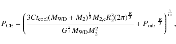
![]() ). The required equations for classical magnetic braking are given in Schreiber & Gänsicke (2003)
). The required equations for classical magnetic braking are given in Schreiber & Gänsicke (2003)![]() . For the Hurley et al. (2002) prescription of disrupted magnetic braking normalized by Davis et al. (2008) we obtain
. For the Hurley et al. (2002) prescription of disrupted magnetic braking normalized by Davis et al. (2008) we obtain
|
(1) |
with
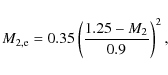
|
(2) |
for
![\begin{figure}
\par\includegraphics[width=9cm,clip]{13658fg1-a.ps}\includegraphics[width=9cm,clip]{13658fg1-b.ps}
\vspace*{4.5mm}
\end{figure}](/articles/aa/full_html/2010/12/aa13658-09/img54.png)
|
Figure 1:
Observed, present-day (bottom) and reconstructed post-CE (middle and top) orbital period distributions (left: logarithmic scale, right:
linear scale) for two different prescriptions of magnetic braking. The
well-defined sample of SDSS-PCEBs is shown in black while the gray
distribution represents the entire WDMS PCEB population (IK Peg is
not present in the right panel of this figure due to its long period
compared with the rest of the sample). There is no significant
difference between the two populations. The observed distributions as
well as the reconstructed zero-age PCEB distributions show a strong
peak at |
| Open with DEXTER | |
In Tables A.1 and A.2 we list the stellar and binary parameters of the PCEBs in our sample as well as their cooling age (
![]() )
and the orbital period the PCEB had at the end of the CE phase (
)
and the orbital period the PCEB had at the end of the CE phase (
![]() ). The corresponding orbital period distributions are shown in Fig. 1.
As most of the observed PCEBs are relatively young and most of our
PCEBs have low-mass secondary stars for which gravitational radiation
is assumed to be the only sink of angular momentum, the reconstructed
zero age post-CE distribution of orbital periods is not dramatically
different from the observed distribution. In addition, the
distributions of the systematically identified SDSS PCEBs (black
histogram in Fig. 1) do not
differ significantly from the distribution of previously known PCEBs
that have been identified through various channels (Schreiber & Gänsicke 2003).
In the following sections we use the zero-age PCEB parameter
reconstructed with the disrupted magnetic braking prescription as given
by Hurley et al. (2002) and normalized by Davis et al. (2008).
After reconstructing the post-CE evolution, we can now concentrate on
discussing implications for theories of CE evolution that can be drawn
from our sample.
). The corresponding orbital period distributions are shown in Fig. 1.
As most of the observed PCEBs are relatively young and most of our
PCEBs have low-mass secondary stars for which gravitational radiation
is assumed to be the only sink of angular momentum, the reconstructed
zero age post-CE distribution of orbital periods is not dramatically
different from the observed distribution. In addition, the
distributions of the systematically identified SDSS PCEBs (black
histogram in Fig. 1) do not
differ significantly from the distribution of previously known PCEBs
that have been identified through various channels (Schreiber & Gänsicke 2003).
In the following sections we use the zero-age PCEB parameter
reconstructed with the disrupted magnetic braking prescription as given
by Hurley et al. (2002) and normalized by Davis et al. (2008).
After reconstructing the post-CE evolution, we can now concentrate on
discussing implications for theories of CE evolution that can be drawn
from our sample.
4 CE equations
It is generally assumed that the outcome of the CE phase can be
approximated by equating the binding energy of the envelope and the
change in orbital energy, and by scaling this equation with an
efficiency ![]() ,
i.e.
,
i.e.

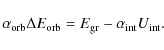
where
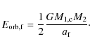
The final orbital energy
![]() is always calculated as the orbital energy between the core of the primary (
is always calculated as the orbital energy between the core of the primary (
![]() )
and the secondary (
)
and the secondary (![]() )
at the final separation (
)
at the final separation (![]() )
)
In contrast, different descriptions exist for the gravitational energy and the initial orbital energy. Some authors (e.g. de Kool 1990; Webbink 1984; Podsiadlowski et al. 2003) calculate the gravitational energy as being between the envelope mass (
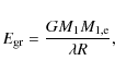
where
As in Kiel & Hurley (2006), we will refer to this as the PRH (Podsiadlowski-Rappaport-Han) formulation.
Another formulation (e.g. Yungelson et al. 1994; Iben & Livio 1993)
takes the binding energy as being between the envelope mass and the
combined mass of the core of the primary and the secondary star
and the initial orbital energy as the orbital energy between the core of the primary and the secondary at the initial binary separation
We will refer to this as the ILY (Iben-Livio-Yungelson) formulation.
Finally there is another scheme, used in the binary star evolution (hereafter BSE) code presented by Hurley et al. (2002), that takes the gravitational energy in the same way as in the PRH formulation (Eq. (5)) and the initial orbital energy as in the ILY formulation (Eq. (8)). We will refer to this as the BSE formulation. We compare the results obtained with the three formulations in Sect. 6.
5 The reconstruction algorithm
As in NT05, we determined the possible masses and radii of the progenitors of the WDs in all the PCEBs listed in Tables A.1 and A.2 from fits to detailed stellar-evolution models. We assumed that the observed WD mass (
![]() )
is equal to the core mass of the giant progenitor (
)
is equal to the core mass of the giant progenitor (
![]() )
at the onset of mass transfer and used the equations from Hurley et al. (2000) to calculate the luminosities
)
at the onset of mass transfer and used the equations from Hurley et al. (2000) to calculate the luminosities ![]() an radii
an radii ![]() of all giant stars that have exactly such a core mass. We did this for initial masses
of all giant stars that have exactly such a core mass. We did this for initial masses ![]() of
of
![]() up
to the mass for which the initial core mass, i.e. the core mass at the
end of the main sequence, is larger than the observed WD mass. We also
included possible progenitors in the Hertzsprung gap (HG) with initial
masses greater than 1.2
up
to the mass for which the initial core mass, i.e. the core mass at the
end of the main sequence, is larger than the observed WD mass. We also
included possible progenitors in the Hertzsprung gap (HG) with initial
masses greater than 1.2
![]() (to ensure a convective envelope). Because we used equations from Hurley et al. (2000)
for the different evolutionary stages instead of running the code, we
set mass dependent luminosity limits for the progenitors in different
evolutionary phases. For stars in the HG we required the luminosity to
be between the luminosity at the top of the main sequence and the
luminosity at the base of the first giant branch (FGB) (i.e.
(to ensure a convective envelope). Because we used equations from Hurley et al. (2000)
for the different evolutionary stages instead of running the code, we
set mass dependent luminosity limits for the progenitors in different
evolutionary phases. For stars in the HG we required the luminosity to
be between the luminosity at the top of the main sequence and the
luminosity at the base of the first giant branch (FGB) (i.e.
![]() ). For the FGB, the luminosity should be between the luminosity at the base and at the end of the FGB phase respectively (i.e.
). For the FGB, the luminosity should be between the luminosity at the base and at the end of the FGB phase respectively (i.e.
![]() ).
For the early asymptotic giant branch (EAGB), we required the
luminosity to be between the luminosity at the base of the AGB and the
luminosity of the second dredge-up (i.e.
).
For the early asymptotic giant branch (EAGB), we required the
luminosity to be between the luminosity at the base of the AGB and the
luminosity of the second dredge-up (i.e.
![]() ).
Finally, for the second AGB (SAGB, i.e. after the second dredge-up) we
required the luminosity to be lower than the peak luminosity of the
first thermal pulse according to Eq. (29) in Izzard et al. (2004). For all possible progenitors we also required
).
Finally, for the second AGB (SAGB, i.e. after the second dredge-up) we
required the luminosity to be lower than the peak luminosity of the
first thermal pulse according to Eq. (29) in Izzard et al. (2004). For all possible progenitors we also required
![]() to be greater than a critical value (
to be greater than a critical value (
![]() ), neccessary to have a CE according to Tout et al. (1997, their Eq. (33)) or greater than 3.2 for a progenitor in the HG.
), neccessary to have a CE according to Tout et al. (1997, their Eq. (33)) or greater than 3.2 for a progenitor in the HG.
After obtaining the mass and radius of a possible WD progenitor with a
core mass equal to the measured WD mass, we assumed that the giant
radius was equal to the Roche-lobe radius at the onset of mass
transfer. Because the secondary mass is assumed to remain constant
during the CE phase, this allows us to determine the orbital separation
just before the CE phase. The remaining quantities in the CE equation
are then the CE efficiency ![]() and the binding energy parameter
and the binding energy parameter ![]() ,
and we can derive
,
and we can derive
![]() for each possible progenitor. In other words, from Roche geometry and the energy equation, we get one value for
for each possible progenitor. In other words, from Roche geometry and the energy equation, we get one value for
![]() for each parameter set consisting of the progenitor mass, core mass (=
current WD mass), secondary mass (= current secondary mass), and final
orbital period (
for each parameter set consisting of the progenitor mass, core mass (=
current WD mass), secondary mass (= current secondary mass), and final
orbital period (
![]() ). In this way we obtain a range of values for
). In this way we obtain a range of values for
![]() for each system that corresponds to a range of possible progenitor masses
for each system that corresponds to a range of possible progenitor masses ![]() .
.
6 Comparing CE prescriptions
Before discussing below what we might be able to learn from
reconstructing the new and much larger sample of PCEBs, we compare here
the results obtained with the three formulations used to describe the
CE evolution (Sect. 4). Each horizontal line in Fig. A.1 represents possible values of
![]() for different masses of the progenitor for a given WD and secondary
mass. As in NT05, the different lines for each object represent
different values of the WD mass within
for different masses of the progenitor for a given WD and secondary
mass. As in NT05, the different lines for each object represent
different values of the WD mass within
![]() from the best-fit value (or within the error given in Table A.1 and A.2 in case it exceeds
from the best-fit value (or within the error given in Table A.1 and A.2 in case it exceeds
![]() ).
Values obtained for FGB progenitors are shown in black, while AGB
progenitors are in blue (see the electronic version of the paper for a
color version). We did not find any possible progenitor on the HG
phase.
).
Values obtained for FGB progenitors are shown in black, while AGB
progenitors are in blue (see the electronic version of the paper for a
color version). We did not find any possible progenitor on the HG
phase.
Solutions for most of the non-SDSS PCEBs are also given in NT05
(their Fig. 6). Comparing their results with those shown in the
left panel of Fig. A.1
one finds that the two reconstruction algorithms give very similar
results with the only notable difference that we generally find
slightly more solutions for a given system. This is because our grid of
progenitor masses is finer by a factor of ten (step size
![]() instead of
instead of
![]() ).
).
Comparing the three panels of Fig. A.1 it becomes obvious that the results obtained with the PRH and BSE algorithm are almost identical, with
![]() being a little but not significantly lower for the BSE scheme. There
are, however, significant differences between those two formulations
and the ILY scheme, which gives by far the lowest values. This is easy
to understand as the ILY formulation predicts much lower values for the
gravitational energy than the PRH prescription. We also note that the
ILY version of
being a little but not significantly lower for the BSE scheme. There
are, however, significant differences between those two formulations
and the ILY scheme, which gives by far the lowest values. This is easy
to understand as the ILY formulation predicts much lower values for the
gravitational energy than the PRH prescription. We also note that the
ILY version of
![]() does not contain the structural parameter
does not contain the structural parameter ![]() .
Hence, we are in fact plotting
.
Hence, we are in fact plotting ![]() for this formulation. In general, it is difficult - if not impossible -
to judge which of the three algorithms for the initial conditions of CE
evolution should be used. In any case, much of the physics is contained
in the parameters
for this formulation. In general, it is difficult - if not impossible -
to judge which of the three algorithms for the initial conditions of CE
evolution should be used. In any case, much of the physics is contained
in the parameters ![]() and
and ![]() .
As most calculations presented in the literature are based on the PRH
or the BSE formalism, we will use the BSE formulation in the following
sections to facilitate the comparison of our results with those
obtained by other authors.
.
As most calculations presented in the literature are based on the PRH
or the BSE formalism, we will use the BSE formulation in the following
sections to facilitate the comparison of our results with those
obtained by other authors.
7 The binding energy of the envelope
The structural parameter ![]() has generally been taken as a constant (typically
has generally been taken as a constant (typically ![]() 0.5).
Detailed stellar models taking into account the structure of the
envelope show that this is a reasonable assumption as long as the
internal energy of the envelope is ignored. In this case one obtains
0.5).
Detailed stellar models taking into account the structure of the
envelope show that this is a reasonable assumption as long as the
internal energy of the envelope is ignored. In this case one obtains
![]() .
However, according to e.g. Dewi & Tauris (2000); Podsiadlowski et al. (2003),
.
However, according to e.g. Dewi & Tauris (2000); Podsiadlowski et al. (2003),
![]() is not a very realistic assumption if a fraction of the internal energy
of the envelope supports the process of envelope ejection. In this
case, especially the extended envelopes of luminous AGB stars can
be very loosely bound, i.e. reaching values of
is not a very realistic assumption if a fraction of the internal energy
of the envelope supports the process of envelope ejection. In this
case, especially the extended envelopes of luminous AGB stars can
be very loosely bound, i.e. reaching values of
![]() .
This is mainly due to the recombination-energy term. It is still not
entirely clear whether this energy indeed contributes to unbind the
envelope of the donor or if it is entirely radiated away (see e.g. Han et al. 2003; Soker & Harpaz 2003,
for further discussion). However, the internal energy of the envelope
might be a very important factor to explain the existence of long
orbital period systems, and we therefore follow Han et al. (1995), who introduced a parameter
.
This is mainly due to the recombination-energy term. It is still not
entirely clear whether this energy indeed contributes to unbind the
envelope of the donor or if it is entirely radiated away (see e.g. Han et al. 2003; Soker & Harpaz 2003,
for further discussion). However, the internal energy of the envelope
might be a very important factor to explain the existence of long
orbital period systems, and we therefore follow Han et al. (1995), who introduced a parameter ![]() th
(between 0 and 1) to characterize the fraction of the internal
energy that is used to expell the CE. Using this, and calling the
parameter
th
(between 0 and 1) to characterize the fraction of the internal
energy that is used to expell the CE. Using this, and calling the
parameter
![]() (as it includes not only the thermal energy, but also the radiation and
the recombination energy), the equation for the standard
(as it includes not only the thermal energy, but also the radiation and
the recombination energy), the equation for the standard ![]() -formalism becomes
-formalism becomes
Alternatively one can revise
|
(10) |
Detailed calculations of this expression have been performed by various authors (e.g. Dewi & Tauris 2000; Podsiadlowski et al. 2003)
who demonstrate that the binding energy depends significantly on the
mass of the giant, its evolutionary state, and of course,
![]() .
Clearly, to include the effect of the internal energy and the structure
of the envelope in the simple energy equation (Eq. (3)) one may equate
.
Clearly, to include the effect of the internal energy and the structure
of the envelope in the simple energy equation (Eq. (3)) one may equate
![]() with the parametrized binding energy
with the parametrized binding energy
![]() from Eq. (5), keeping
from Eq. (5), keeping ![]() variable. The latest version of the BSE code includes an algorithm that computes
variable. The latest version of the BSE code includes an algorithm that computes ![]() in this way.
in this way.
![]() has been calculated using detailed stellar models from Pols et al. (1998) and approximated with analytical fits (Pols, priv. commun.). Using this algorithm
has been calculated using detailed stellar models from Pols et al. (1998) and approximated with analytical fits (Pols, priv. commun.). Using this algorithm ![]() is no longer a constant but depends on the mass, the evolutionary state
of the mass donor, and on the fraction of the internal energy used to
expel the envelope, i.e.
is no longer a constant but depends on the mass, the evolutionary state
of the mass donor, and on the fraction of the internal energy used to
expel the envelope, i.e.
![]() .
Note that the exact definition of the core radius that separates the
ejected envelope from the condensed core region in the primary is of
major importance for high-mass progenitors on the FGB (Tauris & Dewi 2001; van der Sluys et al. 2006).
As we mostly find low-mass progenitors on the FGB the exact definition
of the core radius (and hence of the core mass) can be assumed to be of
minor importance here.The prescription of
.
Note that the exact definition of the core radius that separates the
ejected envelope from the condensed core region in the primary is of
major importance for high-mass progenitors on the FGB (Tauris & Dewi 2001; van der Sluys et al. 2006).
As we mostly find low-mass progenitors on the FGB the exact definition
of the core radius (and hence of the core mass) can be assumed to be of
minor importance here.The prescription of ![]() used in this work is based on the core-envelope boundary being defined
as the mass shell where the hydrogen mass fraction becomes less
than 10%.
used in this work is based on the core-envelope boundary being defined
as the mass shell where the hydrogen mass fraction becomes less
than 10%.
In the next sections we assume the efficiency of using the internal
energy of the envelope and the orbital energy to expell the envelope to
be equal, i.e. we use values of ![]() that include a fraction
that include a fraction
![]() .
Hence, the given values of
.
Hence, the given values of ![]() should be interpreted as the fraction of the total energy that is used
to expell the envelope, independent of whether this energy has to be
transferred from the orbit to the envelope or was already present in
the envelope as internal energy.
should be interpreted as the fraction of the total energy that is used
to expell the envelope, independent of whether this energy has to be
transferred from the orbit to the envelope or was already present in
the envelope as internal energy.
In Fig. A.2 we plot the possible values of ![]() for each PCEB in our sample assuming
for each PCEB in our sample assuming
![]() (left), calculating
(left), calculating ![]() with the BSE algorithm but without internal energy (center), and including a fraction
with the BSE algorithm but without internal energy (center), and including a fraction
![]() of the internal energy (right). Our results indicate that the structural parameter is quite well approximated by assuming
of the internal energy (right). Our results indicate that the structural parameter is quite well approximated by assuming
![]() for
FGB progenitors (in black) because there is hardly any difference
between the black lines in the three panels. However, the effect of
calculating
for
FGB progenitors (in black) because there is hardly any difference
between the black lines in the three panels. However, the effect of
calculating ![]() and including the internal energy is of utmost importance for AGB progenitors: the blue lines move towards lower values of
and including the internal energy is of utmost importance for AGB progenitors: the blue lines move towards lower values of ![]() especially if a fraction of the internal energy is assumed to
contribute to the energy budget of CE evolution. The effect is most
obvious for IK Peg because we only find a solution with
especially if a fraction of the internal energy is assumed to
contribute to the energy budget of CE evolution. The effect is most
obvious for IK Peg because we only find a solution with
![]() if the internal energy is included. This result perfectly agrees with Davis et al. (2010). In addition, the internal energy becomes important especially for long orbital period systems - exactly as suggested by Webbink (2008).
if the internal energy is included. This result perfectly agrees with Davis et al. (2010). In addition, the internal energy becomes important especially for long orbital period systems - exactly as suggested by Webbink (2008).
Inspecting the right panel of Fig. A.2
in more detail, it becomes obvious that including the internal energy
allows us to find solutions for all the systems in a small range of CE
efficiencies, i.e.
![]() (vertical lines). The upper limit of this range (
(vertical lines). The upper limit of this range (
![]() )
is defined by systems with massive WD (so they have progenitors on the
AGB) and short orbital periods after the CE phase. In contrast,
the lower limit (
)
is defined by systems with massive WD (so they have progenitors on the
AGB) and short orbital periods after the CE phase. In contrast,
the lower limit (
![]() )
is given by systems with FGB progenitors (i.e. those with low-mass WDs).
)
is given by systems with FGB progenitors (i.e. those with low-mass WDs).
8  versus
As mentioned above, NT05 used a similar algorithm to reconstruct the
CE phase of double WDs and PCEBs. The problem they encountered can be
summarized as follows: during the first CE phase of virtually all
double WDs and for three alleged PCEBs (AY Cet, S1040 and
IK Peg) the observed binary separation is too large, requiring a
physically unrealisticly high or even a negative efficiency. NT05
therefore proposed to use the angular momentum conservation instead of
the energy conservation because they find the angular momentum relation
in agreement with the observed binary separations of double WDs and all
the PCEBs in their sample. The alternative angular momentum algorithm
for CE evolution (the so called ![]() -algorithm) is described by
-algorithm) is described by
where
![]() is the relative change in angular momentum and
is the relative change in angular momentum and
![]() is the relative change in mass. At first glance, the fact that all the
unexplained double WDs and the three alleged critical PCEBs have
reasonable solutions for
is the relative change in mass. At first glance, the fact that all the
unexplained double WDs and the three alleged critical PCEBs have
reasonable solutions for ![]() appears to be very attractive. Moreover, the obtained values of
appears to be very attractive. Moreover, the obtained values of ![]() cluster in a rather small range of values, i.e.
cluster in a rather small range of values, i.e.
![]() ,
raising hope for a new and universal prescription of CE evolution. However, this turned out to be an illusion as Webbink (2008)
recently showed that energy conservation is much more constraining the
outcome of CE evolution. Indeed, a final energy state lower than the
initial one requires the loss of angular momentum while the opposite is
not necessarily true. In addition, Webbink (2008) showed that the ratio of final to initial orbital separation is extremely sensitive to
,
raising hope for a new and universal prescription of CE evolution. However, this turned out to be an illusion as Webbink (2008)
recently showed that energy conservation is much more constraining the
outcome of CE evolution. Indeed, a final energy state lower than the
initial one requires the loss of angular momentum while the opposite is
not necessarily true. In addition, Webbink (2008) showed that the ratio of final to initial orbital separation is extremely sensitive to ![]() in the range of values proposed by NT05.
in the range of values proposed by NT05.
Our large and representative sample of PCEBs now allows us to test both
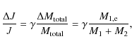
algorithms and to evaluate their predictive power. In Fig. A.3 we show the values of ![]() (left) and
(left) and ![]() (right) for all possible progenitors of the PCEBs in our sample. The binding energy parameter
(right) for all possible progenitors of the PCEBs in our sample. The binding energy parameter ![]() has been calculated with the BSE code including internal energy. All
the PCEBs in our sample can be simultaneously reproduced with
has been calculated with the BSE code including internal energy. All
the PCEBs in our sample can be simultaneously reproduced with ![]() in the range 0.2-0.3 (vertical lines in the left panel). The right
panel shows that indeed literally all systems can be reconstructed with
in the range 0.2-0.3 (vertical lines in the left panel). The right
panel shows that indeed literally all systems can be reconstructed with
![]() (vertical lines).
(vertical lines).
In Fig. A.4 we investigate the effect of constraining ![]() on the possible range of values for
on the possible range of values for ![]() and vice versa. In the left panel we show the values of
and vice versa. In the left panel we show the values of ![]() requesting
requesting
![]() ,
while on the right hand side we show the values of
,
while on the right hand side we show the values of ![]() if
if
![]() .
Apparently, requesting
.
Apparently, requesting ![]() to lie in a small range of values does not very much constrain the values obtained for
to lie in a small range of values does not very much constrain the values obtained for ![]() .
We still find the solutions for
.
We still find the solutions for ![]() covering basically the entire parameter space, i.e.
covering basically the entire parameter space, i.e.
![]() .
This confirms the suggestion of Webbink (2008) that virtually all possible configurations can be explained with similar values of
.
This confirms the suggestion of Webbink (2008) that virtually all possible configurations can be explained with similar values of ![]() ,
which questions the predictive power of the new algorithm.
,
which questions the predictive power of the new algorithm.
In contrast to this, fixing ![]() provides strong constraints on
provides strong constraints on ![]() .
The values we obtain for
.
The values we obtain for ![]() seem to have a clear dependency on the evolutionary stage of the WD
progenitor. It is almost constant for progenitors in the same
evolutionary stage, being higher for FGB progenitors and smaller for
AGB progenitors. This finding has a straightforward physical
interpretation: the envelope of a giant star is more tightly bound on
the FGB and less bound on the AGB, where it is more expanded
(especially on the second AGB). The value of
seem to have a clear dependency on the evolutionary stage of the WD
progenitor. It is almost constant for progenitors in the same
evolutionary stage, being higher for FGB progenitors and smaller for
AGB progenitors. This finding has a straightforward physical
interpretation: the envelope of a giant star is more tightly bound on
the FGB and less bound on the AGB, where it is more expanded
(especially on the second AGB). The value of ![]() represents the ratio of the relative amount of angular momentum loss to
the relative amount of mass loss. Hence, the different values of
represents the ratio of the relative amount of angular momentum loss to
the relative amount of mass loss. Hence, the different values of ![]() may just reflect the simple fact that expelling a tightly (loosely)
bound envelope requires to extract more (less) angular momentum per
unit mass.
may just reflect the simple fact that expelling a tightly (loosely)
bound envelope requires to extract more (less) angular momentum per
unit mass.
Once more, the findings described above perfectly agree with the results obtained by Webbink (2008), i.e. we need to constrain ![]() to
predict the outcome of CE evolution. In addition, the internal energy
of the envelope seems to play an important role. Taking this into
account in the energy equation leads to two classes of solutions in the
angular momentum equation.
to
predict the outcome of CE evolution. In addition, the internal energy
of the envelope seems to play an important role. Taking this into
account in the energy equation leads to two classes of solutions in the
angular momentum equation.
9 Should
be constant?
![\begin{figure}
\par\includegraphics[width=7cm]{13658fg6-a.ps}\includegraphics[width=7cm]{13658fg6-b.ps}
\vspace*{3.5mm}
\end{figure}](/articles/aa/full_html/2010/12/aa13658-09/img100.png)
|
Figure 2:
Weighted mean values of |
| Open with DEXTER | |
In most binary population synthesis models of WDMS (e.g. Willems & Kolb 2004) but also of soft X-ray transients (Kiel et al. 2008; Yungelson & Lasota 2008) or extreme horizontal branch stars (Han et al. 2002),
the CE efficiency is assumed to be constant. Analyzing our sample of
PCEBs consisting of WDs and low-mass main-sequence stars we find that
we can reconstruct the evolutionary history of all systems assuming a
constant value
![]() .
.
An important question is now whether we should expect ![]() to be constant for all types of PCEBs. First steps exploring this have been made by Politano & Weiler (2007), Davis et al. (2008,2010) who recently speculated that instead of being constant,
to be constant for all types of PCEBs. First steps exploring this have been made by Politano & Weiler (2007), Davis et al. (2008,2010) who recently speculated that instead of being constant, ![]() may depend on the mass of the secondary star or on the final orbital
separation as spiraling-in deeper into the envelope may significantly
affect the efficiency of the ejection process.
may depend on the mass of the secondary star or on the final orbital
separation as spiraling-in deeper into the envelope may significantly
affect the efficiency of the ejection process.
We here follow Davis et al. (2008)
and evaluate the formation probability for each possible progenitor of
each PCEB in our sample. The number of primaries with masses in the
range
![]() is given by
is given by
![]() where
where
![]() is given by the initial mass function (IMF):
is given by the initial mass function (IMF):
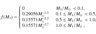
(Kroupa et al. 1993). The probability that a binary forms with a certain initial orbital separation
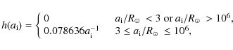
(Davis et al. 2008). The formation probability for each progenitor is then given by
In Fig. 6 we plot the weighted mean value of ![]() for
each system (colored points) versus the mass of the secondary star
(left) and the orbital period the PCEB had at the end of the CE phase
(right). Black vertical lines represent the full range of possible
values of
for
each system (colored points) versus the mass of the secondary star
(left) and the orbital period the PCEB had at the end of the CE phase
(right). Black vertical lines represent the full range of possible
values of ![]() .
Again, we distinguish between progenitors in different evolutionary
stages. Red points indicate systems with progenitors on the FGB, while
blue points are for progenitors on the AGB. Given the uncertainties in
the WD masses, some systems have possible progenitors in more than one
evolutionary stage. For those cases, we separately computed the average
for the different type of progenitors. Finally, dashed horizontal lines
indicate
.
Again, we distinguish between progenitors in different evolutionary
stages. Red points indicate systems with progenitors on the FGB, while
blue points are for progenitors on the AGB. Given the uncertainties in
the WD masses, some systems have possible progenitors in more than one
evolutionary stage. For those cases, we separately computed the average
for the different type of progenitors. Finally, dashed horizontal lines
indicate
![]() and 0.3. There seems to be no dependence of
and 0.3. There seems to be no dependence of ![]() on the mass of the secondary star or on the period, but a large scatter around
on the mass of the secondary star or on the period, but a large scatter around
![]() .
.
This finding remains if we assume alternative initial mass
distributions. We tested for two other probability distributions
assuming that the masses of the binary components are correlated. We
used
![]() and
and
![]() ,
where
,
where
![]() .
In both cases we obtained very similar results, i.e., a large scatter and no relation between
.
In both cases we obtained very similar results, i.e., a large scatter and no relation between ![]() and
and ![]() or
or
![]() .
Although there seems to be no correlation between
.
Although there seems to be no correlation between ![]() and the mass of the secondary or the final period, there is a clear relation between the averaged mean values of
and the mass of the secondary or the final period, there is a clear relation between the averaged mean values of ![]() and the evolutionary state of the progenitor. Systems with FGB progenitors tend to have weighted mean values
and the evolutionary state of the progenitor. Systems with FGB progenitors tend to have weighted mean values
![]() ,
while the obtained mean efficiencies for systems with AGB progenitors are much smaller, i.e.
,
while the obtained mean efficiencies for systems with AGB progenitors are much smaller, i.e.
![]() .
This is easily explained if one remembers that the internal energy
becomes very important for progenitors on the AGB moving the whole
range of possible values of
.
This is easily explained if one remembers that the internal energy
becomes very important for progenitors on the AGB moving the whole
range of possible values of ![]() towards smaller values (see Sect. 7). It is essential to recall here that the given values of
towards smaller values (see Sect. 7). It is essential to recall here that the given values of ![]() represent the fraction of the total energy that is used to expell the
envelope. In other words, the same fraction of internal and orbital
energy are used, i.e.
represent the fraction of the total energy that is used to expell the
envelope. In other words, the same fraction of internal and orbital
energy are used, i.e.
![]() .
However, one could also point out that the orbital energy must first be
transferred to the envelope (presumably as thermal energy), in contrast
to the energy already present in the envelope and that this would give
rise to a different
.
However, one could also point out that the orbital energy must first be
transferred to the envelope (presumably as thermal energy), in contrast
to the energy already present in the envelope and that this would give
rise to a different ![]() for the two. Indeed, the systematically lower weighted mean values of
for the two. Indeed, the systematically lower weighted mean values of ![]() for AGB progenitors may reflect different efficiencies for the orbital and internal energy. If
for AGB progenitors may reflect different efficiencies for the orbital and internal energy. If
![]() is small, the required
is small, the required
![]() will increase especially for systems with AGB progenitor. So, an alternative to
will increase especially for systems with AGB progenitor. So, an alternative to
![]() might be
might be
![]() and
and
![]() but
but
![]() .
A detailed discussion of this alternative possibility is beyond the scope of this paper though.
.
A detailed discussion of this alternative possibility is beyond the scope of this paper though.
As a final remark we emphasize that the weighted mean values discussed
above are lacking a physical meaning. We used these values here only to
test for possible dependencies of ![]() that are missing in the energy equation, which does not seem to be the case. Therefore,
that are missing in the energy equation, which does not seem to be the case. Therefore,
![]() or at least
or at least
![]() and
and
![]() const.,
which corresponds to the assumption that the most important
dependencies are included in the used energy equation remains the
currently most reasonable prescription.
const.,
which corresponds to the assumption that the most important
dependencies are included in the used energy equation remains the
currently most reasonable prescription.
10 Discussion
The results obtained in the previous sections can be summarized as
follows: For all systems in our sample, which is the largest sample of
one specific type of PCEBs that is currently available, we find
possible progenitors assuming energy conservation if the internal
energy of the envelope is taken into account. For each individual
system the possible solutions cover rather broad ranges of values for
the CE efficiency ![]() .
However, there exists only a small range of values, i.e.
.
However, there exists only a small range of values, i.e.
![]() for which we find solutions for all the systems in our sample. This
means that, if a universal value for the CE efficiency does exist, it
should lie in this range. A plausible alternative to such a universal
value for
for which we find solutions for all the systems in our sample. This
means that, if a universal value for the CE efficiency does exist, it
should lie in this range. A plausible alternative to such a universal
value for ![]() is to assume that the fraction of the orbital energy exceeds the
fraction of the internal energy that is used to expell the envelope,
i.e.
is to assume that the fraction of the orbital energy exceeds the
fraction of the internal energy that is used to expell the envelope,
i.e.
![]() .
In addition, we have shown that the energy budget constrains the
outcome of CE evolution much more than the alternative angular momentum
equation. In this section we discuss our results in the context of
recent theoretical and observational results in the field of close
compact binary formation and evolution.
.
In addition, we have shown that the energy budget constrains the
outcome of CE evolution much more than the alternative angular momentum
equation. In this section we discuss our results in the context of
recent theoretical and observational results in the field of close
compact binary formation and evolution.
10.1 Hydrodynamical simulations
Soon after Paczynski (1976) outlined the basic ideas of CE evolution, the first hydrodynamical simulations in one dimension were carried out (Meyer & Meyer-Hofmeister 1979; Taam et al. 1978). Based on these early studies two and three dimensional models have been developed in the last decades (e.g. Bodenheimer & Taam 1984; Sandquist et al. 2000; Taam & Bodenheimer 1989). For a recent review see e.g. Taam & Ricker (2006).
The most important findings of hydrodynamical simulations of CE
evolution are perhaps the relatively short duration of CE evolution (![]() 1000 yrs)
and the preference of ejecting matter in the orbital plane. In
addition, as most particles are predicted to leave the CE with
velocities exceeding the minimum escape speed, the predicted CE
efficiency is less than
1000 yrs)
and the preference of ejecting matter in the orbital plane. In
addition, as most particles are predicted to leave the CE with
velocities exceeding the minimum escape speed, the predicted CE
efficiency is less than ![]() ,
i.e.
,
i.e.
![]() .
This result agrees quite well with our finding of
.
This result agrees quite well with our finding of
![]() .
However, one should note that current hydrodynamical simulations still
cannot follow the entire CE evolution basically because of the large
ranges of timescales and length scales that have to be numerically
resolved. Therefore, even the most detailed hydrodynamical simulations
still have to be considered as rather rough approximations.
.
However, one should note that current hydrodynamical simulations still
cannot follow the entire CE evolution basically because of the large
ranges of timescales and length scales that have to be numerically
resolved. Therefore, even the most detailed hydrodynamical simulations
still have to be considered as rather rough approximations.
10.2 Binary population synthesis
An alternative way to constrain the CE efficiency is to perform binary population studies and compare the predictions with the observed properties of PCEBs. These simulations have become popular in last 10-20 years and have been carried out for a large variety of different PCEB populations. We here briefly review the main results.
10.2.1 WDMS binaries
The population of WDMS binaries has been first simulated by de Kool (1992) and de Kool & Ritter (1993). de Kool & Ritter (1993)
incorporated observational selection effects to compare their
predictions with the - very small and biased - observed populations
they had at hand. Interestingly, for
![]() and
and ![]() randomly taken from the IMF they predict PCEB orbital period
distributions rather similar to the observed distribution (see
Sect. 3). However, the selection effects applied by de Kool & Ritter (1993)
have been designed for blue color surveys such as the Palomar Green
survey and are not applicable to our new SDSS PCEB sample. In addition,
one should take into account that the approximations to stellar
evolution used by de Kool & Ritter (1993)
have been much cruder than the models that are available today and that
they did not include the internal energy of the envelope.
randomly taken from the IMF they predict PCEB orbital period
distributions rather similar to the observed distribution (see
Sect. 3). However, the selection effects applied by de Kool & Ritter (1993)
have been designed for blue color surveys such as the Palomar Green
survey and are not applicable to our new SDSS PCEB sample. In addition,
one should take into account that the approximations to stellar
evolution used by de Kool & Ritter (1993)
have been much cruder than the models that are available today and that
they did not include the internal energy of the envelope.
An update of this early work was carried out by Willems & Kolb (2004), using more detailed analytical fits to stellar evolution (Hurley et al. 2000). Their PCEB orbital period distribution peaks at about one day, i.e. at a significantly longer period than the observed sample. However, one should note that Willems & Kolb (2004) computed formation models for PCEBs, but did not follow the subsequent angular momentum loss by magnetic braking and gravitational radiation. In addition, no observational biases are incorporated in their preditions. Hence, we advocate caution when comparing the predictions of Willems & Kolb (2004) with observed samples.
Full binary population studies of PCEBs have been performed by Politano & Weiler (2006,2007). They tested different formulations of ![]() and discussed the influence on the predicted distributions. The resulting orbital period distributions peak at
and discussed the influence on the predicted distributions. The resulting orbital period distributions peak at
![]() days
and the overall shape does not change significantly for different
prescriptions of the CE efficiency. Again, as observational selection
effects have not been incorporated, it is difficult, if not impossible,
to compare the predicted distributions with the measured orbital period
distributions shown in Fig. 1.
days
and the overall shape does not change significantly for different
prescriptions of the CE efficiency. Again, as observational selection
effects have not been incorporated, it is difficult, if not impossible,
to compare the predicted distributions with the measured orbital period
distributions shown in Fig. 1.
Most recently, Davis et al. (2010)
published a work presenting comprehensive population synthesis studies
of PCEBs. Perhaps most importantly, for the first time the PCEB
population has been simulated including variable values of ![]() .
Comparing their predictions with the observations, Davis et al. (2010) find a disagreement in the orbital period distributions, i.e. the predicted distributions peak at
.
Comparing their predictions with the observations, Davis et al. (2010) find a disagreement in the orbital period distributions, i.e. the predicted distributions peak at
![]() day declining smoothly at longer periods, while observations indicate a rather steep decline at
day declining smoothly at longer periods, while observations indicate a rather steep decline at
![]() day. However, Davis et al. (2010)
compared their predictions with a small sample of PCEBs identified
through various detection channels. Thanks to our concentrated
follow-up of WDMS binaries from SDSS, the number of known PCEBs has
increased by more than a factor of two, and this new SDSS PCEB sample
is less affected by observational biases (Gänsicke et al. 2010, in
prep). In addition, the parameter space explored by Davis et al. (2010) is still rather small. While the CE efficiency has in general been varied over a wide range of values (
day. However, Davis et al. (2010)
compared their predictions with a small sample of PCEBs identified
through various detection channels. Thanks to our concentrated
follow-up of WDMS binaries from SDSS, the number of known PCEBs has
increased by more than a factor of two, and this new SDSS PCEB sample
is less affected by observational biases (Gänsicke et al. 2010, in
prep). In addition, the parameter space explored by Davis et al. (2010) is still rather small. While the CE efficiency has in general been varied over a wide range of values (
![]() ), only one model with variable values of
), only one model with variable values of ![]() assuming
assuming ![]() has been calculated. Finally, one should keep in mind that Davis et al. (2010) interpolated the tables provided by Dewi & Tauris (2000) to determine
has been calculated. Finally, one should keep in mind that Davis et al. (2010) interpolated the tables provided by Dewi & Tauris (2000) to determine ![]() ,
which probably leads to underestimating
,
which probably leads to underestimating ![]() for large radii.
for large radii.
We conclude that binary population synthesis (BPS) simulations using
![]() and including a proper treatment of
and including a proper treatment of ![]() do not yet exist. Hence, it might not be too surprising that predicted
period distributions disagree with the observation. Reducing
do not yet exist. Hence, it might not be too surprising that predicted
period distributions disagree with the observation. Reducing ![]() and incorporating the internal energy should lead to predicting less systems with
and incorporating the internal energy should lead to predicting less systems with
![]() day.
Therefore we anticipate that applying our results may bring theory and
observations into agreement. In addition, the next generation of BPS
simulations should take into account observational biases as detailed
as possible. The importance of this might be indicated by the basic
agreement between the predictions by de Kool & Ritter (1993) and our observed sample.
day.
Therefore we anticipate that applying our results may bring theory and
observations into agreement. In addition, the next generation of BPS
simulations should take into account observational biases as detailed
as possible. The importance of this might be indicated by the basic
agreement between the predictions by de Kool & Ritter (1993) and our observed sample.
10.2.2 Extreme horizontal branch stars
Extreme horizontal branch stars (EHB, also known as hot subdwarfs) are helium-burning stars with very thin hydrogen envelopes (Saffer et al. 1994; Heber et al. 1986). To explain the formation of these stars several scenarios have been discussed mostly based on single-star evolution (e.g. Kilkenny et al. 1997; Green et al. 1986). However, as most EHB stars appear to be members of close binary systems, the binary-formation channel proposed by Han et al. (2002,2003) has become a popular alternative. These authors favored a rather high efficiency (
![]() )
when compared to the value we obtain from our sample. However, one should note that Han et al. (2003) did not explore the full parameter space and did not generally exclude lower values of
)
when compared to the value we obtain from our sample. However, one should note that Han et al. (2003) did not explore the full parameter space and did not generally exclude lower values of ![]() .
.
An interesting option to constrain ![]() might be to measure the binary fraction of EHB stars in globular clusters. Moni Bidin et al. (2006) find the binary fraction in NGC 6752 to be much lower (
might be to measure the binary fraction of EHB stars in globular clusters. Moni Bidin et al. (2006) find the binary fraction in NGC 6752 to be much lower (![]() 4%) than in the field (
4%) than in the field (![]() 70%). As speculated by Moni Bidin et al. (2008) and confirmed later by Han (2008) and Moni Bidin et al. (2009)
this can be explained within the binary-formation scenario, as the
binary fraction among EHB stars in clusters is expected to
decrease with time. According to Han (2008) the
binary fraction - age relation is rather sensitive to the assumed CE
efficiency. First results seem to favor high values of
70%). As speculated by Moni Bidin et al. (2008) and confirmed later by Han (2008) and Moni Bidin et al. (2009)
this can be explained within the binary-formation scenario, as the
binary fraction among EHB stars in clusters is expected to
decrease with time. According to Han (2008) the
binary fraction - age relation is rather sensitive to the assumed CE
efficiency. First results seem to favor high values of ![]() .
However, significantly more measurements of the binary fractions among
EHB stars in globular clusters are required to derive clear
constraints.
.
However, significantly more measurements of the binary fractions among
EHB stars in globular clusters are required to derive clear
constraints.
10.2.3 Low-mass X-ray binaries
The efficiency of CE evolution is of outstanding importance in the
context of compact binaries descending from more massive stars too. For
example, the existence of low-mass X-ray binaries (LMXBs) in our galaxy
has been difficult to explain within the CE picture as low-mass
companions appear to be unable to unbind the envelope of a massive
primary star (Podsiadlowski et al. 2003) and one therefore expects most systems to merge instead of forming a LMXB. As shown by Podsiadlowski et al. (2003), the predicted formation rate of LMXBs is much lower than indicated by observations even for ![]() .
This is explained by the huge binding energy of envelopes around massive cores, i. e.
.
This is explained by the huge binding energy of envelopes around massive cores, i. e.
![]() .
As a solution for this problem, Kiel & Hurley (2006) proposed a reduced mass-loss for helium stars and brought into agreement binary populations synthesis and observations for
.
As a solution for this problem, Kiel & Hurley (2006) proposed a reduced mass-loss for helium stars and brought into agreement binary populations synthesis and observations for
![]() (but see also Yungelson & Lasota 2008). In any case, current models seem to be unable to reproduce the observed population of LMXBs assuming a rather low value of
(but see also Yungelson & Lasota 2008). In any case, current models seem to be unable to reproduce the observed population of LMXBs assuming a rather low value of
![]() as we find for our sample of PCEBs. This indicates that either the
efficiency is different for LMXBs or that the uncertainties in
evolutionary models of very massive late AGB stars strongly affect
the predictions of BPS.
as we find for our sample of PCEBs. This indicates that either the
efficiency is different for LMXBs or that the uncertainties in
evolutionary models of very massive late AGB stars strongly affect
the predictions of BPS.
11 Conclusion
We have developed a new algorithm to reconstruct CE evolution of
PCEB stars. We included a proper treatment of the binding energy
parameter ![]() taking into account the internal energy of the envelope. We have
applied the new algorithm to the largest and most homogeneous sample of
PCEBs currently available. The basic result of this investigation can
be summarized with the following four statements:
taking into account the internal energy of the envelope. We have
applied the new algorithm to the largest and most homogeneous sample of
PCEBs currently available. The basic result of this investigation can
be summarized with the following four statements:
- A reasonable prescription of the CE evolution of PCEBs containing a WD primary and late-M spectral-type secondary is given by the energy equation if the internal energy of the envelope is included.
- The energy equation is much more constraining the outcome of CE evolution and the predictive power of the angular momentum equation is limited.
- If there is a universal value of
 ,
it must be in the range of 0.2-0.3.
,
it must be in the range of 0.2-0.3.
- There are no indications for a dependence of
on the mass of the secondary star or the orbital period.
M.Z. is supported by an ESO studentship. MRS acknowledges support from FONDECYT (grant 1061199). We thank the referee, Marc van der Sluys, for helpfull comments.
References
- Abazajian, K. N., Adelman-McCarthy, J. K., Agüeros, M. A., et al. 2009, ApJS, 182, 543 [NASA ADS] [CrossRef] [Google Scholar]
- Adelman-McCarthy, J. K., Agüeros, M. A., Allam, S. S., et al. 2008, ApJS, 175, 297 [NASA ADS] [CrossRef] [Google Scholar]
- Althaus, L. G., & Benvenuto, O. G. 1997, ApJ, 477, 313 [NASA ADS] [CrossRef] [Google Scholar]
- Bergeron, P., Wesemael, F., Beauchamp, A., et al. 1994, ApJ, 432, 305 [NASA ADS] [CrossRef] [Google Scholar]
- Bleach, J. N., Wood, J. H., Catalán, M. S., et al. 2000, MNRAS, 312, 70 [NASA ADS] [CrossRef] [Google Scholar]
- Bodenheimer, P., & Taam, R. E. 1984, ApJ, 280, 771 [NASA ADS] [CrossRef] [Google Scholar]
- Bragaglia, A., Renzini, A., & Bergeron, P. 1995, ApJ, 443, 735 [NASA ADS] [CrossRef] [Google Scholar]
- Burleigh, M. R., Hogan, E., Dobbie, P. D., Napiwotzki, R., & Maxted, P. F. L. 2006, MNRAS, 373, L55 [Google Scholar]
- Davis, P. J., Kolb, U., Willems, B., & Gänsicke, B. T. 2008, MNRAS, 389, 1563 [NASA ADS] [CrossRef] [Google Scholar]
- Davis, P. J., Kolb, U., & Willems, B. 2010, MNRAS, 403, 179 [NASA ADS] [CrossRef] [Google Scholar]
- de Kool, M. 1990, ApJ, 358, 189 [NASA ADS] [CrossRef] [Google Scholar]
- de Kool, M. 1992, A&A, 261, 188 [NASA ADS] [Google Scholar]
- de Kool, M., & Ritter, H. 1993, A&A, 267, 397 [NASA ADS] [Google Scholar]
- DeGennaro, S., von Hippel, T., Winget, D. E., et al. 2008, AJ, 135, 1 [NASA ADS] [CrossRef] [Google Scholar]
- Dewi, J. D. M., & Tauris, T. M. 2000, A&A, 360, 1043 [NASA ADS] [Google Scholar]
- Drake, A. J., Djorgovski, S. G., Mahabal, A., et al. 2009, ApJ, 696, 870 [NASA ADS] [CrossRef] [MathSciNet] [Google Scholar]
- Fulbright, M. S., Liebert, J., Bergeron, P., & Green, R. 1993, ApJ, 406, 240 [NASA ADS] [CrossRef] [Google Scholar]
- Green, R. F., Richstone, D. O., & Schmidt, M. 1978, ApJ, 224, 892 [NASA ADS] [CrossRef] [Google Scholar]
- Green, R. F., Schmidt, M., & Liebert, J. 1986, ApJS, 61, 305 [NASA ADS] [CrossRef] [Google Scholar]
- Guinan, E. F., & Sion, E. M. 1984, AJ, 89, 1252 [NASA ADS] [CrossRef] [Google Scholar]
- Han, Z. 2008, A&A, 484, L31 [NASA ADS] [CrossRef] [EDP Sciences] [Google Scholar]
- Han, Z., Podsiadlowski, P., & Eggleton, P. P. 1994, MNRAS, 270, 121 [NASA ADS] [CrossRef] [Google Scholar]
- Han, Z., Podsiadlowski, P., & Eggleton, P. P. 1995, MNRAS, 272, 800 [NASA ADS] [Google Scholar]
- Han, Z., Podsiadlowski, P., Maxted, P. F. L., Marsh, T. R., & Ivanova, N. 2002, MNRAS, 336, 449 [NASA ADS] [CrossRef] [Google Scholar]
- Han, Z., Podsiadlowski, P., Maxted, P. F. L., & Marsh, T. R. 2003, MNRAS, 341, 669 [NASA ADS] [CrossRef] [Google Scholar]
- Heber, U., Kudritzki, R. P., Caloi, V., Castellani, V., & Danziger, J. 1986, A&A, 162, 171 [NASA ADS] [Google Scholar]
- Hillwig, T. C., Honeycutt, R. K., & Robertson, J. W. 2000, AJ, 120, 1113 [NASA ADS] [CrossRef] [Google Scholar]
- Hjellming, M. S. 1989, Ph.D. Thesis, A&A (Illinois Univ. Urbana-Champaign, Savoy) [Google Scholar]
- Hurley, J. R., Pols, O. R., & Tout, C. A. 2000, MNRAS, 315, 543 [NASA ADS] [CrossRef] [Google Scholar]
- Hurley, J. R., Tout, C. A., & Pols, O. R. 2002, MNRAS, 329, 897 [NASA ADS] [CrossRef] [Google Scholar]
- Iben, I. J., & Livio, M. 1993, PASP, 105, 1373 [Google Scholar]
- Izzard, R. G., Tout, C. A., Karakas, A. I., & Pols, O. R. 2004, MNRAS, 350, 407 [NASA ADS] [CrossRef] [Google Scholar]
- Kawka, A., Vennes, S., Dupuis, J., & Koch, R. 2000, AJ, 120, 3250 [NASA ADS] [CrossRef] [Google Scholar]
- Kawka, A., Vennes, S., Dupuis, J., Chayer, P., & Lanz, T. 2008, ApJ, 675, 1518 [NASA ADS] [CrossRef] [Google Scholar]
- Kepler, S. O., & Nelan, E. P. 1993, AJ, 105, 608 [NASA ADS] [CrossRef] [Google Scholar]
- Kiel, P. D., & Hurley, J. R. 2006, MNRAS, 369, 1152 [NASA ADS] [CrossRef] [Google Scholar]
- Kiel, P. D., Hurley, J. R., Bailes, M., & Murray, J. R. 2008, MNRAS, 388, 393 [NASA ADS] [CrossRef] [Google Scholar]
- Kilkenny, D., O'Donoghue, D., Koen, C., Stobie, R. S., & Chen, A. 1997, MNRAS, 287, 867 [NASA ADS] [CrossRef] [Google Scholar]
- Knigge, C. 2006, MNRAS, 373, 484 [NASA ADS] [CrossRef] [Google Scholar]
- Koester, D., Schulz, H., & Weidemann, V. 1979, A&A, 76, 262 [NASA ADS] [Google Scholar]
- Kroupa, P., Tout, C. A., & Gilmore, G. 1993, MNRAS, 262, 545 [NASA ADS] [CrossRef] [Google Scholar]
- Landsman, W., Simon, T., & Bergeron, P. 1993, PASP, 105, 841 [NASA ADS] [CrossRef] [Google Scholar]
- Lanning, H. H., & Pesch, P. 1981, ApJ, 244, 280 [NASA ADS] [CrossRef] [Google Scholar]
- Marsh, T. R. & Duck, S. R. 1996, MNRAS, 278, 565 [NASA ADS] [CrossRef] [Google Scholar]
- Maxted, P. F. L., Marsh, T. R., Moran, C., Dhillon, V. S., & Hilditch, R. W. 1998, MNRAS, 300, 1225 [NASA ADS] [CrossRef] [Google Scholar]
- Maxted, P. F. L., Marsh, T. R., Morales-Rueda, L., et al. 2004, MNRAS, 355, 1143 [NASA ADS] [CrossRef] [Google Scholar]
- Maxted, P. F. L., O'Donoghue, D., Morales-Rueda, L., Napiwotzki, R., & Smalley, B. 2007, MNRAS, 376, 919 [NASA ADS] [CrossRef] [Google Scholar]
- Meyer, F., & Meyer-Hofmeister, E. 1979, A&A, 78, 167 [NASA ADS] [Google Scholar]
- Moni Bidin, C., Moehler, S., Piotto, G., et al. 2006, A&A, 451, 499 [NASA ADS] [CrossRef] [EDP Sciences] [Google Scholar]
- Moni Bidin, C., Catelan, M., & Altmann, M. 2008, A&A, 480, L1 [NASA ADS] [CrossRef] [EDP Sciences] [Google Scholar]
- Moni Bidin, C., Moehler, S., Piotto, G., Momany, Y., & Recio-Blanco, A. 2009, A&A, 498, 737 [NASA ADS] [CrossRef] [EDP Sciences] [Google Scholar]
- Nebot Gómez-Morán, A., Schwope, A. D., Schreiber, M. R., et al. 2009, A&A, 495, 561 [NASA ADS] [CrossRef] [EDP Sciences] [Google Scholar]
- Nelemans, G., & Tout, C. A. 2005, MNRAS, 356, 753 [NASA ADS] [CrossRef] [Google Scholar]
- Nelemans, G., Verbunt, F., Yungelson, L. R., & Portegies Zwart, S. F. 2000, A&A, 360, 1011 [NASA ADS] [Google Scholar]
- O'Brien, M. S., Bond, H. E., & Sion, E. M. 2001, ApJ, 563, 971 [NASA ADS] [CrossRef] [Google Scholar]
- O'Donoghue, D., Koen, C., Kilkenny, D., et al. 2003, MNRAS, 345, 506 [NASA ADS] [CrossRef] [Google Scholar]
- Orosz, J. A., Wade, R. A., Harlow, J. J. B., et al. 1999, AJ, 117, 1598 [NASA ADS] [CrossRef] [Google Scholar]
- Paczynski, B. 1976, in Structure and Evolution of Close Binary Systems, IAU Symp., 73, 75 [Google Scholar]
- Parsons, S. G., Marsh, T. R., Copperwheat, C. M., et al. 2010, MNRAS, 402, 2591 [NASA ADS] [CrossRef] [Google Scholar]
- Podsiadlowski, P., Rappaport, S., & Han, Z. 2003, MNRAS, 341, 385 [NASA ADS] [CrossRef] [Google Scholar]
- Politano, M., & Weiler, K. P. 2006, ApJ, 641, L137 [NASA ADS] [CrossRef] [Google Scholar]
- Politano, M., & Weiler, K. P. 2007, ApJ, 665, 663 [NASA ADS] [CrossRef] [Google Scholar]
- Pols, O. R., Schroder, K.-P., Hurley, J. R., Tout, C. A., & Eggleton, P. P. 1998, MNRAS, 298, 525 [NASA ADS] [CrossRef] [Google Scholar]
- Pyrzas, S., Gänsicke, B. T., Marsh, T. R., et al. 2009, MNRAS, 394, 978 [NASA ADS] [CrossRef] [Google Scholar]
- Rappaport, S., Joss, P. C., & Verbunt, F. 1983, ApJ, 275, 713 [NASA ADS] [CrossRef] [Google Scholar]
- Rebassa-Mansergas, A., Gänsicke, B. T., Rodríguez-Gil, P., Schreiber, M. R., & Koester, D. 2007, MNRAS, 382, 1377 [NASA ADS] [CrossRef] [Google Scholar]
- Rebassa-Mansergas, A., Gänsicke, B. T., Schreiber, M. R., et al. 2008, MNRAS, 390, 1635 [NASA ADS] [Google Scholar]
- Rebassa-Mansergas, A., Gänsicke, B. T., Schreiber, M. R., Koester, D., & Rodríguez-Gil, P. 2010, MNRAS, 402, 620 [NASA ADS] [CrossRef] [Google Scholar]
- Saffer, R. A., Wade, R. A., Liebert, J., et al. 1993, AJ, 105, 1945 [NASA ADS] [CrossRef] [Google Scholar]
- Saffer, R. A., Bergeron, P., Koester, D., & Liebert, J. 1994, ApJ, 432, 351 [NASA ADS] [CrossRef] [Google Scholar]
- Sandquist, E. L., Taam, R. E., & Burkert, A. 2000, ApJ, 533, 984 [NASA ADS] [CrossRef] [Google Scholar]
- Schmidt, G. D., Smith, P. S., Harvey, D. A., & Grauer, A. D. 1995, AJ, 110, 398 [NASA ADS] [CrossRef] [Google Scholar]
- Schreiber, M. R., & Gänsicke, B. T. 2003, A&A, 406, 305 [NASA ADS] [CrossRef] [EDP Sciences] [Google Scholar]
- Schreiber, M. R., Nebot Gomez-Moran, A., & Schwope, A. D. 2007, in ASP Conf. Ser. 372, ed. A. Napiwotzki, & M. R. Burleigh, 459 [Google Scholar]
- Schreiber, M. R., Gänsicke, B. T., Southworth, J., Schwope, A. D., & Koester, D. 2008, A&A, 484, 441 [NASA ADS] [CrossRef] [EDP Sciences] [Google Scholar]
- Schreiber, M. R., Gänsicke, B. T., Rebassa-Mansergas, A., et al. 2010, A&A, 513, L7 [NASA ADS] [CrossRef] [EDP Sciences] [Google Scholar]
- Schwope, A. D., Nebot Gomez-Moran, A., Schreiber, M. R., & Gänsicke, B. T. 2009, A&A, 500, 867 [NASA ADS] [CrossRef] [EDP Sciences] [Google Scholar]
- Soker, N., & Harpaz, A. 2003, MNRAS, 343, 456 [NASA ADS] [CrossRef] [Google Scholar]
- Stauffer, J. R. 1987, AJ, 94, 996 [NASA ADS] [CrossRef] [Google Scholar]
- Taam, R. E., & Bodenheimer, P. 1989, ApJ, 337, 849 [NASA ADS] [CrossRef] [Google Scholar]
- Taam, R. E., & Ricker, P. M. 2006 [arXiv:astro-ph/0611043] [Google Scholar]
- Taam, R. E., Bodenheimer, P., & Ostriker, J. P. 1978, ApJ, 222, 269 [NASA ADS] [CrossRef] [Google Scholar]
- Tappert, C., Gänsicke, B. T., Schmidtobreick, L., et al. 2007, A&A, 474, 205 [NASA ADS] [CrossRef] [EDP Sciences] [Google Scholar]
- Tappert, C., Gänsicke, B. T., Zorotovic, M., et al. 2009, A&A, 504, 491 [NASA ADS] [CrossRef] [EDP Sciences] [Google Scholar]
- Tauris, T. M., & Dewi, J. D. M. 2001, A&A, 369, 170 [NASA ADS] [CrossRef] [EDP Sciences] [Google Scholar]
- Tout, C. A., Aarseth, S. J., Pols, O. R., & Eggleton, P. P. 1997, MNRAS, 291, 732 [NASA ADS] [Google Scholar]
- Townsley, D. M., & Bildsten, L. 2003, ApJ, 596, L227 [NASA ADS] [CrossRef] [Google Scholar]
- Townsley, D. M., & Gänsicke, B. T. 2009, ApJ, 693, 1007 [NASA ADS] [CrossRef] [Google Scholar]
- van den Besselaar, E. J. M., Greimel, R., Morales-Rueda, L., et al. 2007, A&A, 466, 1031 [NASA ADS] [CrossRef] [EDP Sciences] [Google Scholar]
- van der Sluys, M. V., Verbunt, F., & Pols, O. R. 2006, A&A, 460, 209 [NASA ADS] [CrossRef] [EDP Sciences] [Google Scholar]
- Vennes, S., Thorstensen, J. R., & Polomski, E. F. 1999, ApJ, 523, 386 [NASA ADS] [CrossRef] [Google Scholar]
- Webbink, R. F. 1984, ApJ, 277, 355 [NASA ADS] [CrossRef] [Google Scholar]
- Webbink, R. F. 2008, in Astrophysics and Space Science Library, ed. E. F. Milone, D. A. Leahy, & D. W. Hobill, Astrophys. Space Sci. Libr., 352, 233 [Google Scholar]
- Willems, B., & Kolb, U. 2004, A&A, 419, 1057 [NASA ADS] [CrossRef] [EDP Sciences] [Google Scholar]
- Wood, M. A. 1995, in White Dwarfs, ed. D. Koester & K. Werner, LNP No. 443 (Heidelberg: Springer), 41 [Google Scholar]
- Yungelson, L. R. & Lasota, J.-P. 2008, A&A, 488, 257 [NASA ADS] [CrossRef] [EDP Sciences] [Google Scholar]
- Yungelson, L. R., Livio, M., Tutukov, A. V., & Saffer, R. A. 1994, ApJ, 420, 336 [NASA ADS] [CrossRef] [Google Scholar]
Online Material
Appendix A: Data
Table A.1: Properties of the SDSS PCEBs.
Table A.2: Properties of the previously known PCEBs.
![\begin{figure}
\par\includegraphics[width=18cm]{13658fg2.eps}
\end{figure}](/articles/aa/full_html/2010/12/aa13658-09/img136.png)
|
Figure A.1:
Reconstructed values of
|
| Open with DEXTER | |
![\begin{figure}
\par\includegraphics[width=18cm]{13658fg3.eps}
\end{figure}](/articles/aa/full_html/2010/12/aa13658-09/img137.png)
|
Figure A.2:
Reconstructed values of |
| Open with DEXTER | |
![\begin{figure}
\par\includegraphics[width=18cm]{13658fg4.eps}
\end{figure}](/articles/aa/full_html/2010/12/aa13658-09/img138.png)
|
Figure A.3:
Reconstructed values for |
| Open with DEXTER | |
![\begin{figure}
\par\includegraphics[width=18cm]{13658fg5.eps}
\end{figure}](/articles/aa/full_html/2010/12/aa13658-09/img139.png)
|
Figure A.4:
Left panel: reconstructed values of |
| Open with DEXTER | |
Footnotes
- ... efficiency
- Appendix A and Figures 2-5 are only available in electronic form at http://www.aanda.org
- ...Schreiber & Gänsicke (2003)
- We found a typographic error in Eq. (11) in Schreiber & Gänsicke (2003): 9
 should be replaced by 2.
All Tables
Table A.1: Properties of the SDSS PCEBs.
Table A.2: Properties of the previously known PCEBs.
All Figures
|
|
Figure 1:
Observed, present-day (bottom) and reconstructed post-CE (middle and top) orbital period distributions (left: logarithmic scale, right:
linear scale) for two different prescriptions of magnetic braking. The
well-defined sample of SDSS-PCEBs is shown in black while the gray
distribution represents the entire WDMS PCEB population (IK Peg is
not present in the right panel of this figure due to its long period
compared with the rest of the sample). There is no significant
difference between the two populations. The observed distributions as
well as the reconstructed zero-age PCEB distributions show a strong
peak at |
| Open with DEXTER | |
| In the text | |
|
|
Figure 2:
Weighted mean values of |
| Open with DEXTER | |
| In the text | |
|
|
Figure A.1:
Reconstructed values of
|
| Open with DEXTER | |
| In the text | |
|
|
Figure A.2:
Reconstructed values of |
| Open with DEXTER | |
| In the text | |
|
|
Figure A.3:
Reconstructed values for |
| Open with DEXTER | |
| In the text | |
|
|
Figure A.4:
Left panel: reconstructed values of |
| Open with DEXTER | |
| In the text | |
Copyright ESO 2010
Current usage metrics show cumulative count of Article Views (full-text article views including HTML views, PDF and ePub downloads, according to the available data) and Abstracts Views on Vision4Press platform.
Data correspond to usage on the plateform after 2015. The current usage metrics is available 48-96 hours after online publication and is updated daily on week days.
Initial download of the metrics may take a while.