| Issue |
A&A
Volume 520, September-October 2010
Pre-launch status of the Planck mission
|
|
|---|---|---|
| Article Number | A13 | |
| Number of page(s) | 12 | |
| Section | Astronomical instrumentation | |
| DOI | https://doi.org/10.1051/0004-6361/200913054 | |
| Published online | 15 September 2010 | |
Pre-launch status of the Planck mission
Planck pre-launch status: High Frequency Instrument polarization calibration
C. Rosset1,5 -
M. Tristram1,11 -
N. Ponthieu2 -
P. Ade3 -
J. Aumont2,11 -
A. Catalano4,5 -
L. Conversi16 -
F. Couchot1 -
B. P. Crill6,9 -
F.-X. Désert7 -
K. Ganga5 -
M. Giard8 -
Y. Giraud-Héraud5 -
J. Haïssinski1 -
S. Henrot-Versillé1 -
W. Holmes9 -
W. C. Jones6,9,14 -
J.-M. Lamarre4 -
A. Lange6,9![]() -
C. Leroy2,8 -
J. Macías-Pérez7 -
B. Maffei10 -
P. de Marcillac2 -
M.-A. Miville-Deschênes2 -
L. Montier8 -
F. Noviello2 -
F. Pajot2 -
O. Perdereau1 -
F. Piacentini12 -
M. Piat5 -
S. Plaszczynski1 -
E. Pointecouteau8 -
J.-L. Puget2 -
I. Ristorcelli8 -
G. Savini3,15 -
R. Sudiwala3 -
M. Veneziani5,12 -
D. Yvon13
-
C. Leroy2,8 -
J. Macías-Pérez7 -
B. Maffei10 -
P. de Marcillac2 -
M.-A. Miville-Deschênes2 -
L. Montier8 -
F. Noviello2 -
F. Pajot2 -
O. Perdereau1 -
F. Piacentini12 -
M. Piat5 -
S. Plaszczynski1 -
E. Pointecouteau8 -
J.-L. Puget2 -
I. Ristorcelli8 -
G. Savini3,15 -
R. Sudiwala3 -
M. Veneziani5,12 -
D. Yvon13
1 - LAL, Laboratoire de l'Accélerateur Linéaire, CNRS Université Paris 11, Bâtiment 200, Orsay, France
2 - IAS, Institut d'Astrophysique Spatiale, CNRS Université Paris 11, Bâtiment 121, 91405 Orsay, France
3 - Astronomy and Instrumentation Group, Cardiff University, Cardiff, Wales, UK
4 - LERMA, CNRS, Observatoire de Paris, 61 Avenue de l'Observatoire, 75014 Paris, France
5 - APC, Astroparticule et Cosmologie, Université
Paris Diderot, Bâtiment Condorcet, 10 rue Alice Domon et Léonie
Duquet, 75205 Paris Cedex 13, France
6 - Observational Cosmology, California Institute of Technology, Mail code: 367-17, Pasadena, CA 91125, USA
7 - LAOG, Laboratoire d'Astrophysique Observatoire de Grenoble, CNRS, Grenoble, France
8 - CESR, CNRS, 9 Av. du colonel Roche, BP44346, 31038 Toulouse Cedex 4, France
9 - Jet Propulsion Laboratory, California Institute of Technology, Pasadena, CA 91109, USA
10 - The University of Manchester, JBCA, School of Physics and Astronomy, Manchester M13 9PL, UK
11 - LPSC, Laboratoire de Physique Subatomique et Cosmologie, CNRS, Grenoble, France
12 - Dipartimento di Fisica, Universitá di Roma ``La Sapienza'', 00185 Roma, Italy
13 - CEA, Service de Physique des Particules, Saclay, France
14 - Department of Physics, Princeton University, Princeton, NJ 08544, USA
15 - Optical Science Laboratory, University College London, Gower Street, WC1E 6BT London, UK
16 - European Space Astronomy Centre, PO Box 78, 28691 Villanueava de la Cañada (Madrid), Spain
Received 3 August 2009 / Accepted 7 April 2010
Abstract
The High Frequency Instrument of Planck will map the entire
sky in the millimeter and sub-millimeter domain from 100 to
857 GHz with unprecedented sensitivity to polarization (
![]()
![]() 10-6 for P either Q or U and
10-6 for P either Q or U and
![]() K)
at 100, 143, 217 and 353 GHz. It will lead to major
improvements in our understanding of the cosmic microwave background
anisotropies and polarized foreground signals. Planck will make high resolution measurements of the E-mode spectrum (up to
K)
at 100, 143, 217 and 353 GHz. It will lead to major
improvements in our understanding of the cosmic microwave background
anisotropies and polarized foreground signals. Planck will make high resolution measurements of the E-mode spectrum (up to
![]() )
and will also play a prominent role in the search for the faint imprint
of primordial gravitational waves on the CMB polarization.
This paper addresses the effects of calibration of both temperature
(gain) and polarization (polarization efficiency and detector
orientation) on polarization measurements. The specific requirements on
the polarization parameters of the instrument are set and we report on
their pre-flight measurement on HFI bolometers.
We present a semi-analytical method that exactly accounts for the
scanning strategy of the instrument as well as the combination of
different detectors. We use this method to propagate errors through to
the CMB angular power spectra in the particular case of Planck-HFI, and to derive constraints on polarization parameters.
We show that in order to limit the systematic error to 10% of the cosmic variance of the E-mode
power spectrum, uncertainties in gain, polarization efficiency and
detector orientation must be below 0.15%, 0.3% and 1
)
and will also play a prominent role in the search for the faint imprint
of primordial gravitational waves on the CMB polarization.
This paper addresses the effects of calibration of both temperature
(gain) and polarization (polarization efficiency and detector
orientation) on polarization measurements. The specific requirements on
the polarization parameters of the instrument are set and we report on
their pre-flight measurement on HFI bolometers.
We present a semi-analytical method that exactly accounts for the
scanning strategy of the instrument as well as the combination of
different detectors. We use this method to propagate errors through to
the CMB angular power spectra in the particular case of Planck-HFI, and to derive constraints on polarization parameters.
We show that in order to limit the systematic error to 10% of the cosmic variance of the E-mode
power spectrum, uncertainties in gain, polarization efficiency and
detector orientation must be below 0.15%, 0.3% and 1![]() respectively. Pre-launch ground measurements reported in this paper already fulfill these requirements.
respectively. Pre-launch ground measurements reported in this paper already fulfill these requirements.
Key words: space vehicles: instruments - techniques: polarimetric - instrumentation: polarimeters - instrumentation: detectors - cosmic microwave background - submillimeter: general
1 Introduction
The Planck![]() satellite, launched on May 14th, 2009, will map the whole sky in
the range 30-857 GHz. One of the most exciting challenges for Planck
is to measure the polarization anisotropies of the cosmic microwave
background (CMB), which offers a unique way to constrain the energy
scale of inflation.
satellite, launched on May 14th, 2009, will map the whole sky in
the range 30-857 GHz. One of the most exciting challenges for Planck
is to measure the polarization anisotropies of the cosmic microwave
background (CMB), which offers a unique way to constrain the energy
scale of inflation.
CMB polarization can be decomposed into modes of even-parity (E-mode) and odd-parity (B-mode). Gravitational waves generated during inflation (hereafter ``primordial'' gravitational waves) create B-modes with a specific angular power spectrum, whose amplitude is related to the energy scale of inflation. A detection of these ``primordial'' B-modes would therefore provide the first measure of the energy scale of inflation.
E-modes were first detected by DASI in 2002, followed by other ground and balloon-borne experiments (QUaD collaboration: Pryke et al. 2009; Kovac et al. 2002; Readhead et al. 2004; Wu et al. 2007; Montroy et al. 2006) covering a few percent of the sky. These detections are complemented by the WMAP satellite observations of the whole sky (Page et al. 2007). All these measurements have confirmed the existence of an E-mode polarization compatible with the
![]() model, and are compatible with a B-mode polarization of zero. The tensor-to-scalar ratio r parametrizes the amplitude of B-mode polarization. The most stringent upper limit on r is obtained by Komatsu et al. (2009), combining WMAP measurements of TT, TE and EE power spectra with baryon acoustic oscillations and supernovae data. They obtain r<0.22 if the scalar spectral index nS is constant, or r<0.55 if a running spectral index is allowed.
model, and are compatible with a B-mode polarization of zero. The tensor-to-scalar ratio r parametrizes the amplitude of B-mode polarization. The most stringent upper limit on r is obtained by Komatsu et al. (2009), combining WMAP measurements of TT, TE and EE power spectra with baryon acoustic oscillations and supernovae data. They obtain r<0.22 if the scalar spectral index nS is constant, or r<0.55 if a running spectral index is allowed.
Planck has been designed to map the E-mode of
polarization with high precision and good control over the polarization
foreground contamination up to multipoles as large as
![]() .
Planck
may also detect the B-mode polarization
anisotropies, if tensor modes contribute at a level of a few
percent or more of the amplitude of the scalar modes (Efstathiou & Gratton 2009).
However, various
instrumental systematic effects, induced by error on the knowledge of
detector characteristics, may alter these measurements. Most of
the properties of the detectors, such as the gain, time constant,
bandpass and beam, are independent of the sensitivity to linear
polarization. These properties are described in detail in companion
papers (Maffei et al. 2010; Lamarre et al. 2010; Pajot et al. 2010; Tauber et al. 2010a).
In this paper, we study the systematic effects induced by
uncertainties in temperature and polarization calibration (gains,
polarization efficiencies and orientations) on Stokes parameters
and E and B-mode
power spectra. We also report on the ground calibration of the
polarization efficiencies and orientations of High Frequency Instrument
(HFI) detectors. A study of polarization systematics for the Low
Frequency Instrument (LFI) of Planck is presented in Leahy et al. (2010).
.
Planck
may also detect the B-mode polarization
anisotropies, if tensor modes contribute at a level of a few
percent or more of the amplitude of the scalar modes (Efstathiou & Gratton 2009).
However, various
instrumental systematic effects, induced by error on the knowledge of
detector characteristics, may alter these measurements. Most of
the properties of the detectors, such as the gain, time constant,
bandpass and beam, are independent of the sensitivity to linear
polarization. These properties are described in detail in companion
papers (Maffei et al. 2010; Lamarre et al. 2010; Pajot et al. 2010; Tauber et al. 2010a).
In this paper, we study the systematic effects induced by
uncertainties in temperature and polarization calibration (gains,
polarization efficiencies and orientations) on Stokes parameters
and E and B-mode
power spectra. We also report on the ground calibration of the
polarization efficiencies and orientations of High Frequency Instrument
(HFI) detectors. A study of polarization systematics for the Low
Frequency Instrument (LFI) of Planck is presented in Leahy et al. (2010).
The paper is organized as follows. In Sect. 2, we present the polarization sensitive bolometers (PSBs) used by the Planck-HFI and the layout of the focal plane. Section 3 gives the generic expression of the polarized photometric equation and introduces the polarization-related systematic effects discussed in Sect. 4. In Sect. 5, we describe a semi-analytical method to propagate uncertainties on temperature and polarization calibration of detectors up to angular power spectra while exactly accounting for the scanning strategy and the combination of multiple detectors. We apply this method to the Planck-HFI in Sect. 6 and derive requirements on the knowledge of these parameters. Finally, Sect. 7 describes the procedure used to measure polarization parameters of the detectors on ground and compares them to the requirements derived in the previous section.
2 Detectors and focal plane layout
HFI uses bolometric detectors cooled to 100 mK to measure
millimeter-wave radiation. They comprise a micro-mesh absorber in a
form resembling a spider web to reduce cosmic ray interactions (hence
the name spider-web bolometer or SWB, see Yun et al. 2004; Bock et al. 1995),
heated by ohmic power dissipation, and a neutron transmutation doped
(NTD) germanium thermistor that measures the temperature variation.
Polarization is measured with specifically designed polarization
sensitive bolometers (PSBs, see Jones et al. 2003), composed of a pair of bolometers that couple to orthogonal linear polarizations, allowing the measurement of I and (local) Q Stokes
parameters (respectively the sum and difference of the signals of the
two bolometers). The SWBs are only slightly sensitive to
polarization, and PSBs do not perfectly reject the cross-polarization
component. We define precisely the cross-polarization leakage in the
next section. The HFI focal plane is composed of 20 SWBs and
16 PSB pairs, i.e., 32 polarization sensitive
bolometers (see Fig. 1). The PSB pairs are grouped in pairs rotated by ![]() and following the same track on the sky, with the angular separation between associated pairs ranging
from 0 0=
and following the same track on the sky, with the angular separation between associated pairs ranging
from 0 0=![]() 0 .
0 .![]() 5 to 2 0=
5 to 2 0=![]() 0 .
0 .![]() 5. Thus, the difference signal within one pair measures Stokes Q (in some local reference frame) while the difference signal within the other pair measures Stokes U.
Both pairs allow measurements of the total intensity through the sum of
signals. This layout was chosen in order to minimize the noise on the
Stokes parameters and their correlation (Couchot et al. 1999).
5. Thus, the difference signal within one pair measures Stokes Q (in some local reference frame) while the difference signal within the other pair measures Stokes U.
Both pairs allow measurements of the total intensity through the sum of
signals. This layout was chosen in order to minimize the noise on the
Stokes parameters and their correlation (Couchot et al. 1999).
![\begin{figure}
\par\includegraphics[width=8cm,clip]{13054fig1.eps}
\end{figure}](/articles/aa/full_html/2010/12/aa13054-09/img22.png)
|
Figure 1: Sky projection of the Planck-HFI focal plane. The crosses symbolize the polarization sensitive bolometers and indicate the orientation of the two linear polarization measured in each horn. The scanning direction is horizontal in this sketch, so that PSB pairs at same frequency follow the same track on the sky. |
| Open with DEXTER | |
The satellite scans the sky by spinning at 1 rpm. The spin axis remains within 7 0=![]() 0 .
0 .![]() 5 of the anti-solar direction (for a detailed presentation of the Planck scanning strategy, see
Tauber et al. 2010b). The angle between the spin axis and the line of sight is
5 of the anti-solar direction (for a detailed presentation of the Planck scanning strategy, see
Tauber et al. 2010b). The angle between the spin axis and the line of sight is
![]()
![]()
![]() depending on detector position in focal plane. The ecliptic pole
regions are thus much more covered than the equatorial region, both in
terms of number of hits per pixel and in different observation
orientations. This means that around the ecliptic poles, each detector
observes the sky with several focal plane orientations and hence
measures I, Q and U.
In contrast, in the equatorial region, at least three
detectors must be combined to obtain the polarization signal. This is
very different from currently designed ground or balloon-borne
experiments in which the Stokes parameters can be measured using a
single detector. This impacts the propagation of errors, as discussed
in detail in Sect. 5.
depending on detector position in focal plane. The ecliptic pole
regions are thus much more covered than the equatorial region, both in
terms of number of hits per pixel and in different observation
orientations. This means that around the ecliptic poles, each detector
observes the sky with several focal plane orientations and hence
measures I, Q and U.
In contrast, in the equatorial region, at least three
detectors must be combined to obtain the polarization signal. This is
very different from currently designed ground or balloon-borne
experiments in which the Stokes parameters can be measured using a
single detector. This impacts the propagation of errors, as discussed
in detail in Sect. 5.
3 Polarized photometric equation
In this section, we derive the expression for the power received by a PSB. Following Jones's notation (Jones 1941), the polarization state of a plane wave can be described by its transverse electric field
where
|
(2) |
where
The filter can also be described by a Jones matrix, as it is not a depolarizing element in the sense defined by Ditchburn (1976). It is simply given by:
|
(3) |
where
Finally, the beam of both the telescope and the horns is described by a generic Jones matrix,
![]() ,
which depends on both radiation frequency and direction on
the sky. The electric field received by the detector is thus
given by:
,
which depends on both radiation frequency and direction on
the sky. The electric field received by the detector is thus
given by:
|
(4) |
where we have included the matrix R which rotates the incoming radiation from the sky reference frame to the intrument reference frame. The coefficients Jij, with i, j in
The intensity measured by the detector is the sum of the intensities coming from each direction and for each frequency:

|
(5) |
To describe the sky signal, we use the Stokes parameters I, Q, U and V (see, e.g., Born & Wolf 1964):
| (6) |
where I is the intensity, Q and U charaterize the linear polarization and V the circular polarization of the sky radiation. We define analogously the beam Stokes parameters as:
| (7) |
(
where
4 Systematics for polarization
In Eq. (8) each term that couples to one of the Stokes parameters may depend on the direction of observation, ![]() ,
and on frequency in non trivial ways. Several other
instrumental effects could be added to give an accurate description of
a detector measurement, such as its time constant, noise or
pointing errors.
,
and on frequency in non trivial ways. Several other
instrumental effects could be added to give an accurate description of
a detector measurement, such as its time constant, noise or
pointing errors.
The final calibration and analysis of HFI data needs to address all these effects and will rely on both ground and in-flight measurements. This is beyond the scope of this paper. However, some comments can already be made.
HFI beam patterns have been simulated with GRASP (see Maffei et al. 2010; Tauber et al. 2010a) and these simulations have been verified by ground calibration performed by Thales Industries. It was shown that optical cross-polarization and circular polarization ![]() due to telescope were less than 0.1%. Their impact has been studied separately (Rosset et al. 2007).
due to telescope were less than 0.1%. Their impact has been studied separately (Rosset et al. 2007).
We will thus consider in the following an ideal optical system for which
![]() is proportional to the identity matrix resulting in
is proportional to the identity matrix resulting in
![]() and
and
![]() .
Equation (8) therefore simplifies to
.
Equation (8) therefore simplifies to
![\begin{displaymath}%
I_{{\rm det}} \! = \! \frac{1}{2} \iint \tau(\nu) \tilde{I}...
...\cos 2\theta\!+\!U\sin 2\theta)] ~ {\rm d}\Omega {\rm d}\nu.~~
\end{displaymath}](/articles/aa/full_html/2010/12/aa13054-09/img63.png)
Realistic bandpasses and frequency dependence of optical beam coupling terms are non-trivial effects that affect absolute calibration. More specifically, calibration could depend on the electromagnetic spectrum of the source. This is expected to impact component separation. In this work, we focus on systematic effects on CMB polarization and rely on absolute calibration on the CMB dipole, the amplitude f which is known to 0.5% accuracy (Fixsen et al. 1994). We expect to measure in flight the relative gain to an accuracy of better than 0.2%, given the gain stability expected for HFI (i.e. better than WMAP, see Hinshaw et al. 2009). Beam asymmetries and pointing errors couple to the scanning strategy of the instrument. A general framework to assess their impact is presented in Shimon et al. (2008) and O'Dea et al. (2007).
Leaving these effects aside for this work, the measurement of a detector reads:
![\begin{displaymath}%
m = g\Big(I + \rho[ Q\cos2(\psi+\alpha)+U\sin2(\psi+\alpha)]\Big) + n
\end{displaymath}](/articles/aa/full_html/2010/12/aa13054-09/img64.png)
in which n is the noise, g is the total gain,
5 Propagation of errors for polarization calibration
In this section, we propagate errors on gain g, on polarization efficiency ![]() and detector orientation
and detector orientation ![]() (as defined in the previous section) up to Stokes parameters (Sect. 5.1) and angular power spectra (Sect. 5.2).
(as defined in the previous section) up to Stokes parameters (Sect. 5.1) and angular power spectra (Sect. 5.2).
This method applies to all polarization experiments observing with total power detectors such as HFI bolometers. It is close to the approach taken by Shimon et al. (2008) and O'Dea et al. (2007). A similar approach, focused on coherent receivers, was first proposed by Hu et al. (2003). The main difference of the method presented here is that it addresses the specific case of Planck which combines different detectors to determine Q and U.
5.1 Error on Stokes parameters
Given a pixelization of the sky and gathering all samples that fall into the same pixel p in a vector ![]() ,
Eq. (10) generalizes to the usual matrix form:
,
Eq. (10) generalizes to the usual matrix form:
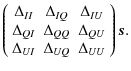
in which
We use a perturbative approach of assumed parameters ![]() ,
,
![]() and
and
![]() (leading to a pointing matrix
(leading to a pointing matrix
![]() )
around their true values g,
)
around their true values g, ![]() and
and ![]() (leading to
A). From Eq. (10), we can see that for Q and U Stokes
parameters, errors on the gain and polarization efficiency are
degenerate. In the following, we use an effective polarization
efficiency
(leading to
A). From Eq. (10), we can see that for Q and U Stokes
parameters, errors on the gain and polarization efficiency are
degenerate. In the following, we use an effective polarization
efficiency
![]() and keep g for intensity only. The actual gain, polarization efficiency and
orientation for a given detector d are therefore
and keep g for intensity only. The actual gain, polarization efficiency and
orientation for a given detector d are therefore
![]() ,
,
![]() and
and
![]() respectively
respectively![]() . Thus, ignoring noise,
. Thus, ignoring noise,
![$\displaystyle \left[ \sum_d \tilde{\mathbf{A}}_d^T\tilde{\mathbf{A}}_d \right]^{-1}
\left[ \sum_d \tilde{\mathbf{A}}_d^T\mathbf{A}_d\right]\vec{s}$](/articles/aa/full_html/2010/12/aa13054-09/img87.png)
![$\displaystyle \left[ \sum_d \tilde{\mathbf{A}}_d^T\tilde{\mathbf{A}}_d \right]^...
...eft[
\sum_d \mathbf{\Lambda}_d(\gamma_d, \epsilon_d, \omega_d)
\right]{\vec s}.$](/articles/aa/full_html/2010/12/aa13054-09/img89.png)
In this expression,
Considering small variations around g,
![]() and
and ![]() ,
we can write the perturbative expansion to first order for both
,
we can write the perturbative expansion to first order for both
![]() ,
,
![]() and
and
![]() :
:
![$\displaystyle \hat{\vec{s}} - \vec{s} =
\left[ \sum_d \tilde{\mathbf{A}}_d^T \t...
...d(\gamma_d, \epsilon_d, \omega_d) - \mathbf{\Lambda}_d(0, 0, 0) \right] \vec{s}$](/articles/aa/full_html/2010/12/aa13054-09/img99.png)
![$\displaystyle \left[ \sum_d \tilde{\mathbf{A}}_d^T \tilde{\mathbf{A}}_d\right]^...
...+\frac{\partial \mathbf{\Lambda}_d}{\partial\omega_d}\omega_d
\right] {\vec s}.$](/articles/aa/full_html/2010/12/aa13054-09/img101.png)
Partial derivatives with respect to gain
The errors
![]() strongly depend on the scanning strategy through the number of hits per
pixel and the distribution of detector orientations. These are
accounted for exactly by taking the scanning strategy of the instrument
and the positions of all detectors, and computing the pointing-related
quantities per pixel on which
strongly depend on the scanning strategy through the number of hits per
pixel and the distribution of detector orientations. These are
accounted for exactly by taking the scanning strategy of the instrument
and the positions of all detectors, and computing the pointing-related
quantities per pixel on which
![]() and
its derivatives depend. This part of the work may be intensive in terms
of memory or disk access requirements depending on which experiment is
being modeled but needs to be performed only once. Then, given a sky
model, the generation of an arbitrary large set of error
maps
and
its derivatives depend. This part of the work may be intensive in terms
of memory or disk access requirements depending on which experiment is
being modeled but needs to be performed only once. Then, given a sky
model, the generation of an arbitrary large set of error
maps
![]() requires fewer resources and
involves only distributions of
requires fewer resources and
involves only distributions of ![]() ,
,
![]() and
and ![]() .
.
Note that in the particular case of an experiment whose scanning
strategy is such that each detector observes each pixel of the map
under angles uniformly distributed over ![]() ,
making a combined
map as in Eq. (12) is equivalent to making one set of I, Q, and U maps
per detector and co-adding them to obtain the final optimal maps of the
experiment. In that case, sums of cosines and sines vanish, which
means that off diagonal terms of
,
making a combined
map as in Eq. (12) is equivalent to making one set of I, Q, and U maps
per detector and co-adding them to obtain the final optimal maps of the
experiment. In that case, sums of cosines and sines vanish, which
means that off diagonal terms of
![]() are zero and Eq. (15) reads simply
are zero and Eq. (15) reads simply
Because of the linearization, the final map is sensitive to the averages of these parameters. If errors are correlated (or identical at worst), they do not average down; if they are randomly distributed around zero mean, they do. These results are in agreement with O'Dea et al. (2007). As we will see in the Sect. 6, this is not the case for HFI, for which none of these simplifications applies.
5.2 Errors on angular power spectra
Following conventions of Zaldarriaga & Seljak (1997), the projection onto spherical harmonics of intensity and polarization reads:
| |
= | ||
| = | |||
| = |
where the
Spherical harmonics transforms are linear, so derivatives of
![]() read
read
We use a simple pseudo-
|
(17) |
This estimator neglects the E-B mixing due to incomplete sky coverage (Lewis et al. 2002) and assumes a cross-power spectrum for which noise bias is null (or if auto-spectra are used, that the noise bias has been previously removed) because their interaction with the systematic effects introduced here are of second order.
Using the previous relations, straightforward algebra leads from Eq. (15) to its counterpart in harmonic space:
![$\displaystyle \left.
{}+~ \frac{\partial^2 \tilde{C}_\ell}{\partial\omega_d\partial\omega_{d'}} \omega_d\omega_{d'}
\right],$](/articles/aa/full_html/2010/12/aa13054-09/img129.png)
where, for
![$\displaystyle \frac{1}{2\ell+1}\sum_{m=-\ell}^{\ell}
\left[
\frac{\partial a^{X...
...}a^Y_{\ell m} + a^{X*}_{\ell m}\frac{\partial a^Y_{\ell m}}{\partial e}
\right]$](/articles/aa/full_html/2010/12/aa13054-09/img132.png)
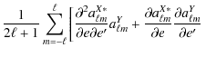
![$\displaystyle \left.{}+ ~
\frac{\partial a^{X*}_{\ell m}}{\partial e'}\frac{\pa...
...a^{X*}_{\ell m}\frac{\partial^2a^Y_{\ell m}}{\partial e\partial e'}\right]\cdot$](/articles/aa/full_html/2010/12/aa13054-09/img135.png)
We ignore cross-terms between different systematic parameters so the previous expressions are only applicable when all but one of the parameters are set to zero. The cross-terms have been checked to be one order of magnitude below the direct terms. Note that we push the perturbative expansion to second order, since E-modes are much larger than B-modes and a second order effect on E-modes has an impact comparable to a first order effect on B-modes.
5.3 Monte-Carlo simulations
We have now everything in hand to perform the semi-analytical estimate of the polarization calibration systematic effects. The method can be described in 5 main steps:
- 1.
- From the scanning strategy of the instrument, for each detector d, project into a map:
 ,
,
 ,
,
 ,
and
,
and
 .
.
- 2.
- With these quantities, compute for each pixel of the map the following 3
 3 matrices:
![$\left[\sum_d \tilde{\mathbf{A}}_d^T\tilde{\mathbf{A}}_d\right]^{-1}$](/articles/aa/full_html/2010/12/aa13054-09/img140.png) ,
,
 ,
and its first and second derivatives.
,
and its first and second derivatives.
- 3.
- Use a simulated CMB sky
 and Eq. (15) to compute partial derivatives
 (up to second order).
- 4.
- Compute all cross-power spectra between
and its derivatives.
- 5.
- Combine these results using gaussian random distributions of
 ,
,
 and
and  (with various rms
  )
in Eq. (18) to obtain the final error on the angular power spectrum.
)
in Eq. (18) to obtain the final error on the angular power spectrum.
6 Application to Planck-HFI focal plane
We apply the method described in the previous section to the Planck-HFI to set requirements on gain, polarization efficiency and orientation. We simulated HEALPix (Górski et al. 2005) full-sky maps
at a resolution of ![]() arcmin (
nside=1024) so that all pixels are seen and each pixel is
uniformly sampled. This avoids the complications of estimating power
spectra on a cut sky when allowing for the same conclusions,
as our power spectrum estimator is not biased in the mean. The
scanning strategy that we use is a realistic simulation of what Planck will actually do in a 14-month mission. The sky signal is pure CMB simulated from the best
arcmin (
nside=1024) so that all pixels are seen and each pixel is
uniformly sampled. This avoids the complications of estimating power
spectra on a cut sky when allowing for the same conclusions,
as our power spectrum estimator is not biased in the mean. The
scanning strategy that we use is a realistic simulation of what Planck will actually do in a 14-month mission. The sky signal is pure CMB simulated from the best
![]() fit to WMAP 5 years data (Dunkley et al. 2009) with r=0.05, supposing the CMB signal to be dominant over foregrounds residuals (at least for intensity and E-mode CMB signals).
fit to WMAP 5 years data (Dunkley et al. 2009) with r=0.05, supposing the CMB signal to be dominant over foregrounds residuals (at least for intensity and E-mode CMB signals).
As described in Sect. 2, the Planck
scanning strategy and focal plane design do not allow the data from a
single PSB pair to provide independent maps of the Stokes
parameters. Here, we will use two PSB pairs calibrated in
intensity and consider small variations around their gain gd = 1, nominal angles
![]() and nominal polarization efficiency
and nominal polarization efficiency
![]() (corresponding to perfect PSB).
(corresponding to perfect PSB).
6.1 Error on Stokes parameter for HFI
We refer to Appendix A
for the explicit form of the derivative terms of the Stokes parameters.
Here, we emphasize the issues specific to HFI. In this case,
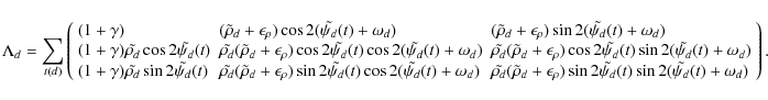
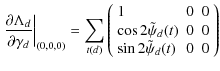
Eq. (15) reads (see Eqs. (A.9)-(A.14))
For gain variations only, non-zero elements of the matrix are given for each pixel, to first order, by
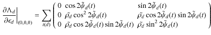
For polarization efficiency only, elements of the matrix are given for each pixel, to first order, by
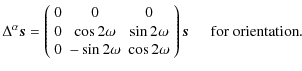
In the case of orientation errors only, to first order,
In these Eqs. (22)-(36), the average is over the samples falling into a given pixel. It depends only on the scanning strategy. Figure 2 shows the angle distribution on the sky for a realistic Planck scanning strategy. Planck shows large inhomogeneities that induce additional terms with respect to the case of a single bolometer.
![\begin{figure}
\par\includegraphics[width=8.5cm,clip]{13054fig2.eps}
\end{figure}](/articles/aa/full_html/2010/12/aa13054-09/img166.png)
|
Figure 2:
Amplitude of the various terms in Eqs. (22)-(36) describing the focal plane angle distribution on the sky for a mock but realistic Planck scanning coverage (HEALPix maps at
nside=1024, Galactic coordinates). From top to bottom:
|
| Open with DEXTER | |
- Leakage from intensity to polarization.
- Error on gain only produces leakage from intensity to polarization (see Eq. (A.8)). This leakage is driven by the relative errors inside a given horn which indicates that an absolute error on the gain (same for all detectors) will not produce any leakage. Neither polarization efficiency nor detector orientation errors induce any leakage from I into polarization Q and U (see Eqs. (A.9)-(A.14)).
- Leakage from polarization to intensity.
- Both polarization efficiency and orientation error produce
leakage from polarization to intensity. It is driven by the
difference of errors within one horn and the relative weight of each
horn depends on the distribution of
 (see Fig. 2).
- Polarization mixing.
- Polarization calibration parameters mix both Q and U. This means that they induce leakage from Q to U through the term
 (and from U to Q through the term
 )
but also alter the amplitude of polarization (
)
but also alter the amplitude of polarization (
 and
and
 ).
If we consider identical errors for each detector, we are in the
limiting case where orientation error induces only leakage (Eqs. (34), (35)) and polarization efficiency only changes the amplitude of polarization (Eqs. (27), (30)) as described by Eq. (16). In the case of Planck-HFI,
and considering independent errors, none of these simplifications
apply. In particular, different parameter averages from one horn
to the other induce both Q and U mixing and amplitude modification.
).
If we consider identical errors for each detector, we are in the
limiting case where orientation error induces only leakage (Eqs. (34), (35)) and polarization efficiency only changes the amplitude of polarization (Eqs. (27), (30)) as described by Eq. (16). In the case of Planck-HFI,
and considering independent errors, none of these simplifications
apply. In particular, different parameter averages from one horn
to the other induce both Q and U mixing and amplitude modification.
6.2 Results for E and B-mode power spectra
The semi-analytical method described in Sect. 5 is able to propagate instrumental errors up to the six CMB power spectra: TT, EE, BB, TE, TB and EB. In this section, we will focus on the E and B-mode power spectra and discuss results obtained for Planck-HFI in case of absolute (Sect. 6.2.1) and relative uncertainties (Sect. 6.2.2). Other spectra (like TB and EB) that are predicted to be null for CMB signal, can be very useful in revealing ``leakage'' due to systematics. However, many systematic effects can produce such leakage, which will make their separate identification very complicated when using only these modes.
6.2.1 Global error over the focal plane/calibration on the sky
Absolute calibration of total power is done using the orbital dipole
that has the same electromagnetic spectrum as the CMB and is not
degenerate with the underlying sky signal as its sign changes after
6 months of observation. From Eqs. (23) and (24), absolute error on the gain g will not produce any leakage in polarization signals:
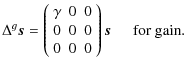
|
(37) |
As far as polarization is concerned, we need a polarized source on the sky. The Crab nebulae, a supernova remnant, is a good candidate as it shows a large polarization emission in the Planck-HFI frequency bands. It has been observed in a wide range of frequencies and shown to have polarization properties stable enough to be a calibrator for polarization experiments. Dedicated observations of this source were done by IRAM at 89 GHz (Aumont et al. 2010). The impact of an approximate knowledge of the polarization sky calibrator leads to a uniform error over the focal plane. In this case, the
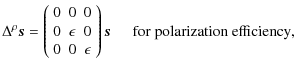
|
(38) |
|
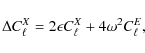
(39) |
In terms of power spectra, an error in polarization efficiencies only affects the amplitude of the E and B power spectra but does not result in leakage from E to B. On the other hand, an error in orientations mixes Q and U maps resulting in both a leakage from E into B (as well as B into E) and a modification of E and B amplitudes. However, as the E-mode signal is far above that of the B-mode in amplitude,
|
(40) |
for X either E or B-mode.
Consequently, for E-mode, the polarization efficiency uncertainty must be
![]() and the orientation uncertainty
and the orientation uncertainty
![]() to obtain less than 1% error on the power spectrum
amplitude. Alternatively, the leakage is kept under 10% of the cosmic variance if
to obtain less than 1% error on the power spectrum
amplitude. Alternatively, the leakage is kept under 10% of the cosmic variance if
![]() and
and
![]() for
for
![]() .
.
To go further and target the B-mode signal, we show that the orientation must be known to better than 1 0=![]() 0 .
0 .![]() 3 (0 0=
3 (0 0=![]() 0 .
0 .![]() 4) in order to keep the leakage from E to B-mode lower than 10% (1%) of the expected
4) in order to keep the leakage from E to B-mode lower than 10% (1%) of the expected
![]() for a tensor-to-scalar ratio of r=0.05 at large angular scales (
for a tensor-to-scalar ratio of r=0.05 at large angular scales (![]() ). The error on its amplitude will be driven by the polarization efficiency uncertainty (
). The error on its amplitude will be driven by the polarization efficiency uncertainty (![]() ).
).
6.2.2 Relative calibration between detectors
As discussed in Sect. 6.1,
there is no generic case concerning the a priori distribution of
errors for polarization parameters on HFI. We therefore performed
10 000 Monte-Carlo simulations to propagate the errors
through to the E and B polarized angular power spectra. Errors were drawn from a gaussian distribution with various dispersions
![]() ,
,
![]() and
and
![]() per detector. We then propagated
those uncertainties through to the E and B angular power spectra.
per detector. We then propagated
those uncertainties through to the E and B angular power spectra.
The results show leakage coming from TT, EE and BB depending on the parameter considered. The gain uncertainty induces leakage from intensity into polarization so
![]() show leakage from TT and TE spectra (dominated by TT). For polarization efficiency and orientation,
show leakage from TT and TE spectra (dominated by TT). For polarization efficiency and orientation,
![]() is a combination of EE and BB power
spectra with relative weights that depend on the distribution of
uncertainties between the four bolometers considered. Due to
second order terms, the distribution of errors in the angular power
spectra is highly non gaussian, as shown in Figs. 3-5.
is a combination of EE and BB power
spectra with relative weights that depend on the distribution of
uncertainties between the four bolometers considered. Due to
second order terms, the distribution of errors in the angular power
spectra is highly non gaussian, as shown in Figs. 3-5.
![\begin{figure}
\par\includegraphics[width=8.8cm,clip]{13054fig3.eps}
\end{figure}](/articles/aa/full_html/2010/12/aa13054-09/img187.png)
|
Figure 3:
Distribution of
|
| Open with DEXTER | |
![\begin{figure}
\par\includegraphics[width=8.8cm,clip]{13054fig4.eps}
\end{figure}](/articles/aa/full_html/2010/12/aa13054-09/img188.png)
|
Figure 4:
Distribution of
|
| Open with DEXTER | |
![\begin{figure}
\par\includegraphics[width=8.8cm,clip]{13054fig5.eps}
\end{figure}](/articles/aa/full_html/2010/12/aa13054-09/img189.png)
|
Figure 5:
Distribution of
|
| Open with DEXTER | |
We then compare the rms of those distributions for each multipole to the cosmic variance of the E-mode and to an r=0.05 B-mode spectrum with lensing (Figs. 6-8).
![\begin{figure}
\par\includegraphics[width=8.5cm,clip]{13054fig6.eps}
\end{figure}](/articles/aa/full_html/2010/12/aa13054-09/img190.png)
|
Figure 6:
|
| Open with DEXTER | |
![\begin{figure}
\par\includegraphics[width=8.5cm,clip]{13054fig7.eps}
\end{figure}](/articles/aa/full_html/2010/12/aa13054-09/img191.png)
|
Figure 7:
|
| Open with DEXTER | |
![\begin{figure}
\par\includegraphics[width=8.5cm,clip]{13054fig8.eps}
\end{figure}](/articles/aa/full_html/2010/12/aa13054-09/img192.png)
|
Figure 8:
|
| Open with DEXTER | |
Using these results, we can set the requirements for Planck-HFI
on the calibration of gain, polarization efficiency and orientation.
More precisely, we demand that the errors on the temperature and
polarization calibration parameters to be such that the induced leakage
into the
E power spectrum is lower than 10% of the cosmic variance over the multipole range
![]() .
This means that gains must be known to
.
This means that gains must be known to ![]() ,
polarization efficiencies to
,
polarization efficiencies to ![]() and detector orientations to
and detector orientations to
![]() .
.
According to Efstathiou & Gratton (2009), an extended Planck mission should be able to measure gravitational B-mode at a level of r=0.05 and put an upper-limit of r=0.03
when considering
foreground residuals and noise levels. To achieve such a detection
(or upper-limit), the constraints on the calibration
parameters must be much tighter. For this goal, we set the leakage
into B power
spectrum to be 10% of the B-mode model we want to target, for a multipole range from ![]() to 100. With such an hypothesis, we find that the gain precision
should be better than 0.05% and the orientations of the bolometers
should be known to better than 0 0=
to 100. With such an hypothesis, we find that the gain precision
should be better than 0.05% and the orientations of the bolometers
should be known to better than 0 0=![]() 0 .
0 .![]() 75. The leakage due to polarization efficiency into B-mode is very small (see bottom plot in Fig. 7), thus the constraint on the polarization efficiency determination is not relevant in that case (we found 10%).
75. The leakage due to polarization efficiency into B-mode is very small (see bottom plot in Fig. 7), thus the constraint on the polarization efficiency determination is not relevant in that case (we found 10%).
7 Ground measurements
The Planck-HFI polarization calibration on ground was divided into two parts: polarization efficiencies were measured for each detector separately, before focal plane assembly, at the University of Wales in Cardiff in 2005, while orientations of the PSBs with respect to the focal plane were measured during the overall calibration of the Planck HFI in the Saturne cryostat at Orsay, France, in 2006.
7.1 Polarization efficiency ground measurements
Detector-level polarization efficiency measurements were performed in a
2-stage adiabatic demagnetization refrigerator (ADR) at a base
temperature of 200 mK. The ADR was configured to take six
detectors per cooldown (in most cases all of the same optical band
per cooldown). Thermal blocking filters were used at the 4 K,
77 K and 300 K stages of the testbed. The
anti-reflective coating on the cryostat window was matched to the
optical band under test. The window, of 125 mm diameter, and all
the thermal blockers were sized such that they filled the beams. The
polarization source was a rotating polarizer grid positioned over an
extended temperature-controlled black body source of 75 mm
diameter running at 126![]() C.
The final source aperture was 70 mm in diameter. The
mechanical structure of the source was fully clad with non-rotating
Eccosorb (type AN-72). The source was positioned approximately
690 mm from the cryostat window, tilted 4 0=
C.
The final source aperture was 70 mm in diameter. The
mechanical structure of the source was fully clad with non-rotating
Eccosorb (type AN-72). The source was positioned approximately
690 mm from the cryostat window, tilted 4 0=![]() 0 .
0 .![]() 8
off the optical axis, and mechanically chopped at 6 Hz. The
experimental setup was fully surrounded with Eccosorb (type AN-72)
while the data were recorded. Data were recorded in a step and sample
fashion over five
full rotations of the polarizer grid with a 4
8
off the optical axis, and mechanically chopped at 6 Hz. The
experimental setup was fully surrounded with Eccosorb (type AN-72)
while the data were recorded. Data were recorded in a step and sample
fashion over five
full rotations of the polarizer grid with a 4![]() step size and a 4 s integration time.
step size and a 4 s integration time.
Detailed results are given in the appendix in Tables B.1 and B.2 for PSBs and SWBs, respectively. The polarization efficiency of the SWBs is low, as expected, and range between 1.6% and 8.6%. The statistical error is typically 0.5%, and as much as 1.8% for one SWB. The polarization efficiency of the PSBs is typically around 90%, ranging from 84% to 96%, with errors below 0.3%.
7.2 Orientation ground measurements
7.2.1 The calibration setup
The orientation calibration was performed within a 1-m diameter
cryostat cooled to 2 K, to be close to flight conditions
(for a more detailed description of the calibration setup and
photographs, see Pajot et al. 2010).
The detectors were cooled to their nominal operating
temperature, 100 mK. For polarization measurements,
the source (Cold Source 2 or CS2) was a blackbody
at 20 K whose radiation was diluted within a 50 cm
diameter sphere in order to illuminate,
after a reflection from mirror, the full focal plane at once.
The source was modulated by a diapason at a fixed frequency
of 10 Hz. The radiation was linearly polarized by an
aluminum grid deposited on a 138 mm diameter mylar film. The
aluminum strips of the polarizer were 5 ![]() m wide, 5
m wide, 5 ![]() m thick and spaced 5
m thick and spaced 5 ![]() m apart. The Mylar film itself was 10
m apart. The Mylar film itself was 10 ![]() m thick,
with a transmission coefficient greater than 0.9;
the polarization efficiency of the polarizer was measured to be
better than 99.9%, so it can be assumed equal to unity at
HFI frequencies. The polarizer could rotate freely around its axis
using a stepper motor. There are exactly 32 000 steps in one
rotation, so the precision in relative angle is better than 1
m thick,
with a transmission coefficient greater than 0.9;
the polarization efficiency of the polarizer was measured to be
better than 99.9%, so it can be assumed equal to unity at
HFI frequencies. The polarizer could rotate freely around its axis
using a stepper motor. There are exactly 32 000 steps in one
rotation, so the precision in relative angle is better than 1
![]() .
.
7.2.2 Reference for angle measurement
The reference position was defined by a pin fixed to the polarizer,
which was detected by electric contact with a copper strip with a
precision of ![]() motor steps, i.e.
motor steps, i.e. ![]() 0 0=
0 0=![]() 0 .
0 .![]() 06.
We measured the angle of this reference position with respect to the
focal plane using the light of a laser diffracted by the strips of the
polarizer; the diffraction pattern is formed by points aligned
orthogonally to the strips (i.e. parallel to the transmitted
polarization).
06.
We measured the angle of this reference position with respect to the
focal plane using the light of a laser diffracted by the strips of the
polarizer; the diffraction pattern is formed by points aligned
orthogonally to the strips (i.e. parallel to the transmitted
polarization).
Two different methods were used to determine polarization
angles with respect to the focal plane. In the first method, we
measured the orientation with respect to the platform and used the
mechanical position of the instrument with respect to the platform to
get the absolute angle. In the second method, we measured the
angle directly with respect to the instrument. In both cases, we
measured the same angle and checked it was constant across the
polarizer. Both methods gave similar error estimates on the reference
position angle, which can safely be assumed to be lower than 0 0=![]() 0 .
0 .![]() 3:
3:
|
(41) |
7.2.3 Data analysis
For this measurement, the polarizer was rotated by 5![]() steps and signal was inegrated for 20 s at each position. Eight full rotations of the polarizer were performed.
steps and signal was inegrated for 20 s at each position. Eight full rotations of the polarizer were performed.
At each polarizer position, the signal from the source is sinusoidal with a frequency of 10 Hz. It is demodulated fitting a sine curve over a few periods, yielding around 60 independent measurements for each stationary period of 20 s. The average and standard deviation of these 60 measurements give the signal and its error for each 20 s period, for a fixed position of the polarizer. The statistical error was found to be typically below 1% of the signal.
We then fit the signal as a function of the polarizer angle to
estimate the polarization efficiency and the orientation of the
detectors. However, despite the good quality of the polarizer,
we found cross-polarization leakage of around 30%, much
higher than that found in Sect. 7.1,
with the Cardiff measurements: it was probably due to standing
waves between the polarizer and the focal plane and made the detector
polarization efficiency unmeasurable with this setup. The angle that
maximizes the signal gives the orientation of the polarizer; however,
the PSB angle must be given in the horn aperture plane, which
is slightly out of parallel with the polarizer plane. We have performed
ray-tracing simulations to estimate and correct for this geometrical
effect. The corrections lie between -0 0=![]() 0 .
0 .![]() 5 to 0 0=
5 to 0 0=![]() 0 .
0 .![]() 5, and the precision (set by the precision on the
position of the polarizer) is better than 0 0=
5, and the precision (set by the precision on the
position of the polarizer) is better than 0 0=![]() 0 .
0 .![]() 15.
15.
![\begin{figure}
\par\includegraphics[width=8.5cm,clip]{13054fig9.eps}
\end{figure}](/articles/aa/full_html/2010/12/aa13054-09/img201.png)
|
Figure 9: Signal of PSB 100-1b with respect to the angle in the horn aperture plane; each color represents one rotation of the polarizer (8 turns); the signal is fitted using a standard sine curve. The difference exhibits a systematic effect that can be explained by standing waves between the polarizer and the focal plane (see text). |
| Open with DEXTER | |
Figure 9 shows the curve obtained for a PSB at 100 GHz and the difference with the fitted model. The residuals show a 90![]() -periodic
sine curve, which is present in some detectors. Some detectors also
have glitches, reproduced at the same position at each rotation of the
polarizer. These glitches mostly affect the highest two frequency
channels (545 and 857 GHz), i.e., only SWBs. As
-periodic
sine curve, which is present in some detectors. Some detectors also
have glitches, reproduced at the same position at each rotation of the
polarizer. These glitches mostly affect the highest two frequency
channels (545 and 857 GHz), i.e., only SWBs. As
![]() and
and
![]() are orthogonal functions over
are orthogonal functions over ![]() ,
the fitted values for the angle and the polarization efficiency
are unchanged when adding such a term in the fitting model. However, we
cannot exclude that they may be contaminated by a systematic effect
like some other modes (mainly in mode
,
the fitted values for the angle and the polarization efficiency
are unchanged when adding such a term in the fitting model. However, we
cannot exclude that they may be contaminated by a systematic effect
like some other modes (mainly in mode
![]() ).
For example, if the incoming radiation is the sum of two
partially linearly polarized radiations, one with orientation
).
For example, if the incoming radiation is the sum of two
partially linearly polarized radiations, one with orientation ![]() (rotating with the polarizer) and one with fixed orientation
(rotating with the polarizer) and one with fixed orientation ![]() ,
the signal measured by the detector reads:
,
the signal measured by the detector reads:
| |
|||
| (42) |
where
More generally, we can expand the signal as a Fourier series
![]() and fit its coefficients cn (which fulfill the condition
and fit its coefficients cn (which fulfill the condition
![]() ,
as s is a real quantity). The coefficient c2, giving the dependence in
,
as s is a real quantity). The coefficient c2, giving the dependence in
![]() ,
contains the information on polarization efficiency and angle through
its modulus and argument, and is independent of the other modes.
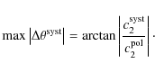
To estimate the error on the polarization angle without relying
on a particular model, we assume that the mode c2 is the sum of two contributions,
,
contains the information on polarization efficiency and angle through
its modulus and argument, and is independent of the other modes.
To estimate the error on the polarization angle without relying
on a particular model, we assume that the mode c2 is the sum of two contributions,
![]() (true polarization signal and induced systematic effect). The maximum systematic error on the angle is then given by:
(true polarization signal and induced systematic effect). The maximum systematic error on the angle is then given by:
|
(43) |
We draw an upper bound on the systematic error by assuming that
|
(44) |
As an independent check, we compared the relative angle between PSBs within each horn (which is close but not exactly equal to 90
The case of SWBs is treated separately, as the statistical error is not negligible in this case (due to the low polarization efficiencies). We performed a similar analysis, taking into account the statistical error. The results are gathered in Table B.2. Note that the SWBs are not meant to be used for polarization measurements.
8 Discussion and conclusion
This paper focuses on the impact of polarized calibration parameters (gain, polarization efficiency and detector orientation) on power spectra in the context of Planck-HFI. We have developed a semi-analytical method that allows us to compute quickly and easily the impact of uncertainties on gain, polarization efficiency and orientation on the E and B-mode power spectra, while exactly accounting for the scanning strategy and the combination of different detectors. We used this method in the particular case of Planck-HFI and derived constraints on the gain, polarization efficiency and detector orientation needed to achieve Planck-HFI's scientific goals.
Planck will use the orbital dipole to calibrate the total power
for each detector. We find that the relative uncertainty on the gain
must be lower than 0.15% to keep systematic error on E-mode power spectrum below 10% of the cosmic variance in the multipole range
![]() .
Given the 0.2% accuracy on relative gain obtained by WMAP (Hinshaw et al. 2009), we expect that HFI can achieve the 0.15% requirements, thanks to the higher gain stability expected for HFI.
.
Given the 0.2% accuracy on relative gain obtained by WMAP (Hinshaw et al. 2009), we expect that HFI can achieve the 0.15% requirements, thanks to the higher gain stability expected for HFI.
We show that the polarization efficiency uncertainty must be
below 0.3% in order to achieve the required sensitivity for the E-mode. The error on the primordial B-mode power spectrum will be
kept below 10% of the signal expected from a tensor-to-scalar ratio r=0.05 in the multipole range
![]() if the polarization efficiency is known to better than 10.3%.
In this paper, we have
presented the results of the ground measurements on HFI PSBs
polarization efficiency, which show an accuracy of 0.3% that
fulfills the requirements for both E and B-modes.
if the polarization efficiency is known to better than 10.3%.
In this paper, we have
presented the results of the ground measurements on HFI PSBs
polarization efficiency, which show an accuracy of 0.3% that
fulfills the requirements for both E and B-modes.
For the polarization orientation, we have distinguished a global
orientation error of the focal plane (which affects identically all
detectors) from a relative error (different for each detector).
For E-modes, we show that the requirement is 2 0=![]() 0 .
0 .![]() 1 on the global orientation knowledge and 1
1 on the global orientation knowledge and 1![]() on the relative orientation to keep the error below 10% of the cosmic variance in the range
on the relative orientation to keep the error below 10% of the cosmic variance in the range
![]() .
Both these requirements are already fulfilled by the ground measurements, in which we found 0 0=
.
Both these requirements are already fulfilled by the ground measurements, in which we found 0 0=![]() 0 .
0 .![]() 3 and 0 0=
3 and 0 0=![]() 0 .
0 .![]() 9 respectively. In order to measure a B-mode signal with a systematic error lower than 10% for a tensor-to-scalar ratio r=0.05, the global orientation must be known to better than 1 0=
9 respectively. In order to measure a B-mode signal with a systematic error lower than 10% for a tensor-to-scalar ratio r=0.05, the global orientation must be known to better than 1 0=![]() 0 .
0 .![]() 2 and the relative orientation at better than 0 0=
2 and the relative orientation at better than 0 0=![]() 0 .
0 .![]() 75.
While the ground measurements fulfill the requirement on global
orientation, the relative orientation knowledge will need to be
improved in flight. For Planck, we plan to use the Crab nebula as the primary polarization calibrator (Aumont et al. 2010),
which will also allow the results presented in this paper to be
cross-checked. The accuracy of the ground measurements of polarization
efficiencies and orientations will allow the E-mode power
spectrum to be measured, with systematic errors lower than 10% of
the cosmic variance, provided that the other sources of systematic
effects are controlled.
75.
While the ground measurements fulfill the requirement on global
orientation, the relative orientation knowledge will need to be
improved in flight. For Planck, we plan to use the Crab nebula as the primary polarization calibrator (Aumont et al. 2010),
which will also allow the results presented in this paper to be
cross-checked. The accuracy of the ground measurements of polarization
efficiencies and orientations will allow the E-mode power
spectrum to be measured, with systematic errors lower than 10% of
the cosmic variance, provided that the other sources of systematic
effects are controlled.
The Planck-HFI instrument (http://hfi.planck.fr/) was designed and built by an international consortium of laboratories, universities and institutes, with important contributions from the industry, under the leadership of the PI institute, IAS at Orsay, France. It was funded in particular by CNES, CNRS, NASA, STFC and ASI. The authors extend their gratitude to the numerous engineers and scientists, who have contributed to the design, development, construction or evaluation of the HFI instrument. The authors are pleased to thank the referee for his/her very useful remarks.
References
- Aumont, A., Conversi, L., Falgarone, E., et al. 2010, A&A, 514, A70 [NASA ADS] [CrossRef] [EDP Sciences] [Google Scholar]
- Bock, J. J., Chen, D., & Mauskopf, P. D. 1995, Space Sci. Rev., 74, 229 [NASA ADS] [CrossRef] [Google Scholar]
- Born, M., & Wolf, E. 1964, Principles of Optics (Pergamon Press) [Google Scholar]
- Couchot, F., Delabrouille, J., Kaplan, J., & Revenu, B. 1999, A&AS, 135, 579 [Google Scholar]
- Ditchburn, R. W. 1976, Light, vol. I (Academic Press) [Google Scholar]
- Dunkley, J., Komatsu, E., Nolta, M. R., et al. 2009, ApJS, 180, 306 [NASA ADS] [CrossRef] [Google Scholar]
- Efstathiou, G., & Gratton, S. 2009, J. Cosmol. Astro-Part. Phys., 6, 11 [Google Scholar]
- Fixsen, D. J., Cheng, E. S., Cottingham, D. A., et al. 1994, ApJ, 420, 445 [NASA ADS] [CrossRef] [Google Scholar]
- Górski, K. M., Hivon, E., Banday, A. J., et al. 2005, ApJ, 622, 759 [NASA ADS] [CrossRef] [Google Scholar]
- Grain, J., Tristram, M., & Stompor, R. 2009, Phys. Rev. D, 79, 123515 [Google Scholar]
- Hinshaw, G., Weiland, J. L., Hill, R. S., et al. 2009, ApJS, 180, 225 [NASA ADS] [CrossRef] [Google Scholar]
- Hu, W., Hedman, M. M., & Zaldarriaga, M. 2003, Phys. Rev. D, 67, 043004 [NASA ADS] [CrossRef] [Google Scholar]
- Jones, R. C. 1941, J. Opt. Soc. Am., 31, 488 [Google Scholar]
- Jones, W. C., Bhatia, R. S., Bock, J. J., & Lange, A. E. 2003, in SPIE Proc., 4855, 227 [Google Scholar]
- Kogut, A., Spergel, D. N., Barnes, C., et al. 2003, ApJS, 148, 161 [NASA ADS] [CrossRef] [MathSciNet] [Google Scholar]
- Komatsu, E., Dunkley, J., Nolta, M. R., et al. 2009, ApJS, 180, 330 [NASA ADS] [CrossRef] [Google Scholar]
- Kovac, J., Leitch, E. M., Pryke, C., et al. 2002, Nature, 420, 772 [NASA ADS] [CrossRef] [PubMed] [Google Scholar]
- Lamarre, J.-M., Puget, J.-L., Ade, P. A. R., et al. 2010, A&A, 520, A9 [NASA ADS] [CrossRef] [EDP Sciences] [Google Scholar]
- Leahy, J. P., Bersanelli, M., D'Arcangelo, O., et al. 2010, A&A, 520, A8 [NASA ADS] [CrossRef] [EDP Sciences] [Google Scholar]
- Lewis, A., Challinor, A., & Turok, N. 2002, Phys. Rev. D, 65, 023505 [NASA ADS] [CrossRef] [Google Scholar]
- Maffei, B., Noviello, F., Murphy, J. A., et al. 2010, A&A, 520, A12 [NASA ADS] [CrossRef] [EDP Sciences] [Google Scholar]
- Montroy, T., Ade, P. A. R., Bock, J. J., et al. 2006, ApJ, 647, 813 [NASA ADS] [CrossRef] [Google Scholar]
- O'Dea, D., Challinor, A., & Johnson, B. R. 2007, MNRAS, 376, 1767 [NASA ADS] [CrossRef] [Google Scholar]
- Page, L., Hinshaw, G., Komatsu, E., et al. 2007, ApJS, 170, 335 [NASA ADS] [CrossRef] [Google Scholar]
- Pajot, F., Ade, P. A. R., Beney, J.-L., et al. 2010, A&A, 520, A10 [NASA ADS] [CrossRef] [EDP Sciences] [Google Scholar]
- QUaD collaboration: Pryke, C., Ade, P., Bock, J., et al. 2009, ApJ, 692, 1247 [NASA ADS] [CrossRef] [Google Scholar]
- Readhead, A. C. S., Myers, S. T., Pearson, T. J., et al. 2004, Science, 306, 836 [NASA ADS] [CrossRef] [PubMed] [Google Scholar]
- Rosset, C., Yurchenko, V., Delabrouille, J., et al. 2007, A&A, 464, 405 [NASA ADS] [CrossRef] [EDP Sciences] [Google Scholar]
- Shimon, M., Keating, B., Ponthieu, N., & Hivon, E. 2008, Phys. Rev. D, 77, 083003 [NASA ADS] [CrossRef] [Google Scholar]
- Tauber, J. A., Noigaard-Nielsen, H. U., Ade, P. A. R., et al. 2010a, A&A, 520, A2 [NASA ADS] [CrossRef] [EDP Sciences] [Google Scholar]
- Tauber, J. A., Mandolesi, N., Pujet, J.-L., et al. 2010b, A&A, 520, A1 [NASA ADS] [CrossRef] [EDP Sciences] [Google Scholar]
- Tristram, M., Macias-Perez, J., Renault, C., & Santos, D. 2005, MNRAS, 358, 833 [NASA ADS] [CrossRef] [Google Scholar]
- Wu, J. H. P., Zuntz, J., Abroe, M. E., et al. 2007, ApJ., 665, 55 [NASA ADS] [CrossRef] [Google Scholar]
- Yun, M., Bock, J. J., Holmes, W., Koch, T., & Lange, A. E. 2004, J. Vac. Sci. Technol. B, 22, 220 [CrossRef] [Google Scholar]
- Zaldarriaga, M., & Seljak, U. 1997, Phys. Rev. D, 55, 1830 [Google Scholar]
Appendix A: Explicit forms of pointing related functions
We write the projection of the signal ![]() into a sky map
into a sky map ![]() as
as
![$\displaystyle \left[ \sum_d \tilde{A}_d^T\tilde{A}_d \right]^{-1}
\left[ \sum_d \tilde{A}_d^TA_d{\vec s} \right]$](/articles/aa/full_html/2010/12/aa13054-09/img219.png)
![$\displaystyle \left[ \sum_d \tilde{A}_d^T\tilde{A}_d \right]^{-1}
\left[
\sum_d \Lambda_d(\gamma_d, \epsilon_d, \omega_d){\vec s}
\right].$](/articles/aa/full_html/2010/12/aa13054-09/img220.png)
Where A is the pointing matrix. In this expression,
|
(A.4) |
Considering small variations around
![$\displaystyle \left[ \sum_d \tilde{A}_d^T \tilde{A}_d \right]^{-1}
\left[ \sum_d \tilde{A}_d^T A_d - \tilde{A}_d^T \tilde{A}_d \right] {\vec s}$](/articles/aa/full_html/2010/12/aa13054-09/img225.png)
![$\displaystyle \left[ \sum_d \tilde{A}_d^T \tilde{A}_d \right]^{-1}
\left[ \sum_d \Lambda_d(\gamma_d, \epsilon_d, \omega_d) - \Lambda_d(0, 0, 0) \right] {\vec s}$](/articles/aa/full_html/2010/12/aa13054-09/img226.png)
![$\displaystyle \left[ \sum_d \tilde{A}_d^T \tilde{A}_d\right]^{-1}
\sum_d \left[...
...ilon_d +
\frac{\partial \Lambda_d}{\partial\omega_d} \omega_d
\right] {\vec s}.$](/articles/aa/full_html/2010/12/aa13054-09/img227.png)
Straightforward generalization to second order reads:
![\begin{displaymath}%
\Delta {\vec s} =
\left[ \sum_d \tilde{A}_d^T \tilde{A}_d...
...bda_d}{\partial e_d \partial e'_d} e_d e'_d
\right] {\vec s}.
\end{displaymath}](/articles/aa/full_html/2010/12/aa13054-09/img228.png)
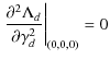
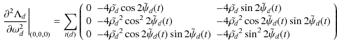
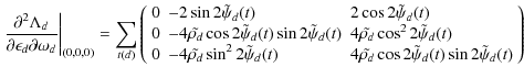
Derivatives of
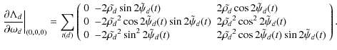
And second order derivatives reads

Appendix B: Polarization efficiencies and angles
Table B.1: Polarization efficiencies and orientations for Planck-HFI PSBs.
Table B.2: Polarization efficiencies and orientations for Planck-HFI SWBs.
Footnotes
- ...Planck
![[*]](/icons/foot_motif.png)
- Planck (http://www.esa.int/Planck) is a project of the European Space Agency (ESA) with instruments provided by two scientific Consortia funded by ESA member states (in particular the lead countries: France and Italy) with contributions from NASA (USA), and telescope reflectors provided in a collaboration between ESA and a scientific Consortium led and funded by Denmark.
- ... respectively
- In the following, when a relation holds for
 ,
,  or
or  ,
we simply write e.
,
we simply write e.
All Tables
Table B.1: Polarization efficiencies and orientations for Planck-HFI PSBs.
Table B.2: Polarization efficiencies and orientations for Planck-HFI SWBs.
All Figures
|
|
Figure 1: Sky projection of the Planck-HFI focal plane. The crosses symbolize the polarization sensitive bolometers and indicate the orientation of the two linear polarization measured in each horn. The scanning direction is horizontal in this sketch, so that PSB pairs at same frequency follow the same track on the sky. |
| Open with DEXTER | |
| In the text | |
|
|
Figure 2:
Amplitude of the various terms in Eqs. (22)-(36) describing the focal plane angle distribution on the sky for a mock but realistic Planck scanning coverage (HEALPix maps at
nside=1024, Galactic coordinates). From top to bottom:
|
| Open with DEXTER | |
| In the text | |
|
|
Figure 3:
Distribution of
|
| Open with DEXTER | |
| In the text | |
|
|
Figure 4:
Distribution of
|
| Open with DEXTER | |
| In the text | |
|
|
Figure 5:
Distribution of
|
| Open with DEXTER | |
| In the text | |
|
|
Figure 6:
|
| Open with DEXTER | |
| In the text | |
|
|
Figure 7:
|
| Open with DEXTER | |
| In the text | |
|
|
Figure 8:
|
| Open with DEXTER | |
| In the text | |
|
|
Figure 9: Signal of PSB 100-1b with respect to the angle in the horn aperture plane; each color represents one rotation of the polarizer (8 turns); the signal is fitted using a standard sine curve. The difference exhibits a systematic effect that can be explained by standing waves between the polarizer and the focal plane (see text). |
| Open with DEXTER | |
| In the text | |
Copyright ESO 2010
Current usage metrics show cumulative count of Article Views (full-text article views including HTML views, PDF and ePub downloads, according to the available data) and Abstracts Views on Vision4Press platform.
Data correspond to usage on the plateform after 2015. The current usage metrics is available 48-96 hours after online publication and is updated daily on week days.
Initial download of the metrics may take a while.