The lag and duration–luminosity relations of gamma-ray burst pulses

S. Boçi; M. Hafizi; R. Mochkovitch

doi:10.1051/0004-6361/201014132

Home

All issues

Volume 519 (September 2010)

A&A, 519 (2010) A76

Full HTML

Free Access

Issue		A&A Volume 519, September 2010


Article Number		A76
Number of page(s)		8
Section		Stellar structure and evolution
DOI		https://doi.org/10.1051/0004-6361/201014132
Published online		15 September 2010

A&A 519, A76 (2010)

The lag and duration-luminosity relations of gamma-ray burst pulses

S. Boçi¹ - M. Hafizi¹ - R. Mochkovitch²

1 - Tirana University, Faculty of Natural Sciences, Tirana, Albania
2 - Institut d'Astrophysique de Paris, UMR 7095 Université Pierre et Marie Curie-Paris 6 - CNRS, 98bis boulevard Arago, 75014 Paris, France

Received 25 January 2010 / Accepted 8 June 2010

Abstract
Context. Relations linking the temporal or/and spectral properties of the prompt emission of gamma-ray bursts (hereafter GRBs) to the absolute luminosity are of great importance as they both constrain the radiation mechanisms and represent potential distance indicators. Here we discuss two such relations: the lag-luminosity relation and the newly discovered duration-luminosity relation of GRB pulses.
Aims. We aim to extend our previous work on the origin of spectral lags, using the duration-luminosity relation recently discovered by Hakkila et al. (2008, ApJ, 677, L81) to connect lags and luminosity. We also present a way to test this relation which has originally been established with a limited sample of only 12 pulses.
Methods. We relate lags to the spectral evolution and shape of the pulses with a linear expansion of the pulse properties around maximum. We then couple this first result to the duration-luminosity relation to obtain the lag-luminosity and lag-duration relations. We finally use a Monte-Carlo method to generate a population of synthetic GRB pulses which is then used to check the validity of the duration-luminosity relation.
Results. Our theoretical results for the lag and duration-luminosity relations are in good agreement with the data. They are rather insensitive to the assumptions regarding the burst spectral parameters. Our Monte Carlo analysis of a population of synthetic pulses confirms that the duration-luminosity relation must be satisfied to reproduce the observational duration-peak flux diagram of BATSE GRB pulses.
Conclusions. The newly discovered duration-luminosity relation offers the possibility to link all three quantities: lag, duration and luminosity of GRB pulses in a consistent way. Some evidence for its validity have been presented but its origin is not easy to explain in the context of the internal shock model.

Key words: gamma-rays bursts: general - radiation mechanisms: non-thermal

1 Introduction

The prompt emission of gamma-ray bursts is characterized by the diversity of the observed temporal profiles. Some bursts show a simple shape with a fast rise followed by a slower decay while others have a complex structure with a succession of pulses which can be overlapping or separated by intervals with almost no emission. Conversely the spectra are more uniform, generally well fitted by two smoothly connected power laws (the so-called Band spectrum; Band et al. 1993). Many studies have tried to link the temporal and spectral properties of bursts with the objective to gain insight into the physical processes governing the prompt emission. Already before and during the BATSE era several relations between hardness and duration (Kouveliotou et al. 1993), intensity (Golenetskii et al. 1983) and fluence (Liang & Kargatis 1996) were found. Following the discovery of the afterglows and the measure of the first redshifts, intrinsic quantities such as the luminosity or the total radiated energy became accessible and new relations appeared: the Amati (Amati et al. 2002) and Ghirlanda (Ghirlanda et al. 2004) relations between the peak energy of the global spectrum and the energy release in gamma-rays (assuming isotropic emission in the Amati relation and corrected for beaming in the Ghirlanda relation), the luminosity-variability relation (Reichart et al. 2001) illustrating the tendency of luminous bursts to be more variable and the lag-luminosity relation (hereafter LLR) discovered by Norris et al. (2000). Spectral lags are a way to quantify the changes in the burst profiles observed in different energy bands. When viewed at high energy, pulses are narrower and peak earlier. Norris et al. (2000) cross-correlated the profiles between BATSE bands 1 and 3 and found that the resulting lags were decreasing with increasing burst peak luminosity. As for the other relations between luminosity and spectral or temporal properties, the LLR offers clues to the physics of the prompt emission but also provides a potential method to evaluate GRB distances from observations at high energy only.

Spectral lags are a direct consequence of the burst spectral evolution since a fixed, constant spectrum, would lead to proportional profiles in all energy bands. In a first paper (Hafizi & Mochkovitch 2007) we computed spectral lags of pulses, defined as the time interval between pulse maximum in two different bands. We obtained an explicit expression for the lags and assuming the validity of an ``Amati-like'' relation between luminosity and the value of $E_{\rm p}$ at pulse maximum we were able to connect lags and luminosity.

Hakkila et al. (2008) have recently reconsidered the LLR and obtained a new relation which applies to individual pulses while the original Norris et al. (2000) LLR considered the burst as a whole. Moreover, they also found a correlation between pulse duration and luminosity (hereafter DLR). These results offer the possibility to directly test and extend our previous work (Hafizi & Mochkovitch 2007). We start in Sect. 2 by comparing to observations our theoretical results for the LLR. Since they rely on the validity of the DLR we propose to test it in Sect. 3 by comparing a synthetic population of GRB pulses to the observed peak flux-duration diagram of a sample of pulses collected by Hakkila & Cumbee (2009). We discuss our results in Sect. 4 and Sect. 5 is the conclusion.

2 The lag-luminosity relation

2.1 Theoretical interpretation

In Paper I (Hafizi & Mochkovitch 2007) we presented a simple analytical model to calculate spectral lags. We recognized that lags were better defined using individual pulses rather than the whole burst profile. Pulses in the same burst can have different lags and Hakkila et al. (2008) have shown that the global lag represents some average where the brightest pulse (which generally has the shortest lag) makes the dominant contribution. Looking for correlation between lag and luminosity it is therefore preferable to consider each pulse separately. Hakkila et al. (2008) obtained

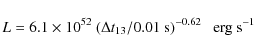
$\begin{displaymath}L=6.1\times 10^{52}\ (\Delta t_{13}/0.01\ {\rm s})^{-0.62}\ \ \ {\rm erg~s}^{-1} \end{displaymath}$

(1)

where L is the peak pulse luminosity and $\Delta t_{13}$ the spectral lag between BATSE bands 1 and 3. This expression is believed to be more directly linked to the physics of the prompt emission than the original one found by Norris et al. (2000)

$\begin{displaymath}L=1.3\times 10^{53}\ (\Delta t_{13}/0.01\ {\rm s})^{-1.15}\ \ \ {\rm erg~s}^{-1} \end{displaymath}$

(2)

where lags were computed by cross-correlation of the full burst profile between the two bands. For individual pulses, spectral lags are more easily estimated from the time difference between the peaks. These ``pulse peak lags'' generally agree with those obtained by cross-correlation and have been used by Hakkila et al. (2008) to get Eq. (1).

$\begin{figure} \par\includegraphics[width=10.4cm,clip]{14132f1.eps} \end{figure}$	Figure 1: Plot of the three functions $f_{13,E_{\rm p}}$ (full line), $-f_{13,\alpha }$ (dotted line) and $-f_{13,\beta }$ (dashed line) for $\alpha =-1$ and $\beta =-2.25$ .
Open with DEXTER

$\begin{figure} \par\includegraphics[width=10.4cm,clip]{14132f2.eps} \end{figure}$

Figure 2:

Ratio of spectral lag over pulse duration as a function of the peak energy at pulse maximum (lower scale) and of the peak luminosity (upper scale) assuming the validity of the Amati-like relation (Eq. (7)). The full lines correspond to ${\dot e}_{\rm p}=-0.5$ and from top to bottom respectively to $\dot a=\dot b=0.2$ , 0.1 and 0. The dashed lines have the same $\dot a$ and $\dot b$ but ${\dot e}_{\rm p}=-0.25$ . The adopted value of the curvature parameter is |C₁|=10.

Open with DEXTER

$\begin{figure} \par\includegraphics[width=10.4cm,clip]{14132f3.eps} \end{figure}$

Figure 3:

Plot of the pulse duration as a function of spectral lag. The full thick line represents our reference model which adopts the Amati-like relation (Eq. (7)) and $\alpha =-1$ , $\beta =-2.25$ , $\dot E=-0.5$ , $\dot a=\dot b=0.1$ and |C₁|=10. The thin lines correspond to nine other cases with different choices of the parameters (see text for details). The squares are the data points of the sample considered in Hakkila et al. (2008).

Open with DEXTER

$\begin{figure} \par\includegraphics[width=10.4cm,clip]{14132f4.eps} \end{figure}$	Figure 4: Theoretical lag-luminosity relation for pulses compared to the data collected by Hakkila et al. (2008). The thick line is the reference case while the thin lines correspond to different model parameters (see Fig. 3 and text for details).
Open with DEXTER

In our theoretical analysis (Hafizi & Mochkovitch 2007) we calculated pulse peak lags from a linear expansion of the pulse shape and spectral properties around the maximum in BATSE band 1 (20-50 keV). Our result directly relates the lag to spectral evolution in a very transparent way. We get

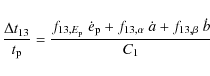
$\begin{displaymath}{\Delta t_{13}\over t_{\rm p}}= {f_{13,E_{\rm p}}~{\dot e}_{\rm p}+ f_{13,\alpha}~{\dot a}+f_{13,\beta}~{\dot b}\over C_1} \end{displaymath}$

(3)

where $t_{\rm p}$ is the pulse duration. The other terms are defined in the following way:

$\begin{displaymath}f_{13,X}={\partial {\rm Log} {\cal F}_{13}\over \partial {\rm... ...m p}}^{50/E_{\rm p}} {\cal B}_{\alpha\beta}(x)~{\rm d}x} \cdot \end{displaymath}$

(4)

Here t₁ is the time of pulse maximum in BATSE band 1 and ${\cal B}_{\alpha\beta}(x)$ is the spectrum shape for which we assumed a Band function (with $x=E/E_{\rm p}$ , $E_{\rm p}$ being the peak energy of the spectrum and $\alpha$ and $\beta$ the two spectral indices at low and high energy). The derivatives ${\dot e}_{\rm p}$ , $\dot a$ and $\dot b$ are respectively given by

$\begin{displaymath}{\dot e}_{\rm p}={{\dot E_{\rm p}}\over E_{\rm p}}~t_{\rm p},... ...a}~t_{\rm p},\ \ {\dot b}={{\dot \beta}\over \beta}~t_{\rm p} \end{displaymath}$

(5)

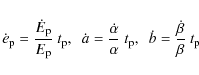
and are evaluated at t=t₁. Finally C₁ is a ``curvature parameter'' for the pulse around maximum. We have

$\begin{displaymath}{C_1\over t_{\rm p}^2}={{\ddot N}_1(t_1)\over N_1(t_1)}\ \ \ \ \ \ (C_1<0) \end{displaymath}$

(6)

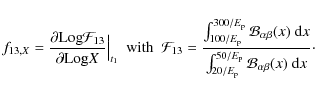
where N₁(t) is the count rate in BATSE band 1.

The functions f_13,X depend on the spectrum parameters $E_{\rm p}$ , $\alpha$ and $\beta$ at pulse maximum while ${\dot e}_{\rm p}$ , $\dot a$ and $\dot b$ represent their evolution. The two remaining quantities in Eq. (1), $t_{\rm p}$ and C₁, are fixed by the pulse shape. They show that spiky pulses (large |C₁|) have shorter lags than broad pulses (small |C₁|) for a given spectral evolution and pulse duration and that short pulses are expected to have short lags, both effects in agreement with observations (Norris & Bonnell 2006; Gehrels et al. 2006; Hakkila et al. 2007). The three functions $f_{13,E_{\rm p}}$ , $f_{13,\alpha}$ and $f_{13,\beta}$ have been represented in Fig. 1 for $\alpha =-1$ and $\beta =-2.25$ which are the central values of the distributions found by Preece et al. (2000) in their study of the spectral properties of bright BATSE bursts. Their behavior can be understood by noting that at large (resp. small) $E_{\rm p}$ values ${\cal F}(E_{\rm p},\alpha,\beta)$ depends on $\alpha$ (resp. $\beta$ ) only. Therefore $f_{13,E_{\rm p}}=\partial {\rm Log} {\cal F}_{13}/ \partial {\rm Log} E_{\rm p}$ mostly contribute at intermediate $E_{\rm p}$ (between BATSE bands 1 and 3) while $f_{13,\alpha}$ (resp. $f_{13,\beta}$ ) dominates at large (resp. small) $E_{\rm p}$ . The resulting ratio $\Delta t_{13}/t_{\rm p}$ has been plotted in Fig. 2 as a function of $E_{\rm p}$ for different values of ${\dot e}_{\rm p}$ , $\dot a$ , $\dot b$ and |C₁|=10.

This value of the curvature parameter as been adopted as representative of a ``typical pulse''. In any case, the results for a different |C₁|are easily obtained by rescaling $\Delta t_{13}/t_{\rm p}$ by a factor 10/|C₁|. As the maximum of $E_{\rm p}$ generally precedes that of the count rate in most pulses we have ${\dot e}_{\rm p}< 0$ . Similarly, the decrease of the spectral indices (spectral softening) begins before pulse maximum implying that $\dot a>0$ and $\dot b>0$ (since $\alpha$ and $\beta$ are negative).

To link spectral lags and luminosity Hafizi & Mochkovitch (2007) have moreover assumed an ``Amati-like relation'' between $E_{\rm p}$ and the pulse peak luminosity of the form

$\begin{displaymath}E_{\rm p}=380\left(L\over 1.6\times 10^{52}\; {\rm erg~s}^{-1}\right)^{0.43}~ {\rm keV}. \end{displaymath}$

(7)

This relation, proposed by Ghirlanda et al. (2005), is expected to be valid at any time contrary to the original Amati relation (Amati et al. 2002) which applies to the burst as a whole. Using Eqs. (3) and (7) it becomes possible to represent $\Delta t_{13}/t_{\rm p}$ as a function of luminosity. The results have also been plotted in Fig. 2. It can be seen that, as long as $\dot a$ and $\dot b$ are not too close to 0, $\Delta t_{13}/t_{\rm p}$ only weakly depends on the luminosity. It is only if the spectral evolution is limited to a decrease of the peak energy (the spectral indices staying constant) that $\Delta t_{13}/t_{\rm p}$ can reach very low values at both high and low luminosities. Since observed bursts show a simultaneous spectral evolution in $E_{\rm p}$ and the spectral indices we expect that $\Delta t_{13}/t_{\rm p}$ will not change much from pulse to pulse in agreement with observations (Hakkila et al. 2008).

A roughly constant value of $\Delta t_{13}/t_{\rm p}$ however raises a problem which was already mentioned in Paper I. If pulses indeed satisfy a lag-luminosity relation with bright pulses having very short lags, some additional parameter has to be correlated to the luminosity. In Paper I we tentatively proposed that pulse curvature could be such a parameter, luminous pulses being spikier and less luminous ones broader. But the recent discovery by Hakkila et al. (2008) of a possible correlation between pulse duration and peak luminosity offers a new perspective which can naturally account for the LLR.

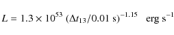
2.2 The duration-luminosity relation of GRB pulses

Hakkila et al. (2008) re-analized the seven BATSE bursts with known redshift considered by Norris et al. (2000) to establish the original LLR but they treated each pulse of these bursts separately. From the 12 selected pulses they obtained a new LLR (Eq. (1)) but also discovered an even tighter relation between duration and luminosity

$\begin{displaymath}L=3.4\times 10^{52}\; t_{\rm p}^{-0.85}\ \ \ \ {\rm erg~s}^{-1}. \end{displaymath}$

(8)

Coupling this to Eq. (3) then provides a very simple way to get the LLR. An important difference with paper I is that we do not necessarily assume the validity of the ``Amati-like relation'' (Eq. (7)) to link $E_{\rm p}$ to the luminosity. Even if $E_{\rm p}$ and L are essentially independent quantities a LLR can still be obtained with the same value of the peak energy at all luminosities. In Figs. 3 and 4 we present the results for both the $\Delta t_{13}$ - $t_{\rm p}$ relation and the LLR. The full heavy line in each diagram corresponds to our reference case which assumes the validity of the Amati-like relation and uses the following values of the parameters: $\alpha =-1$ , $\beta =-2.25$ , ${\dot e}_{\rm p}=-0.5$ , $\dot a=\dot b=0.1$ and |C₁|=10. In addition we plot with thin lines a few other cases: (1) ${\dot e}_{\rm p} =-1$ (other parameters unchanged); (2) ${\dot e}_{\rm p}=-0.25$ ; (3) $\dot a=\dot b=0$ (other parameters unchanged); (4) $\dot a=\dot b=0.2$ ; (5), (6) and (7) no Amati relation but constant $E_{\rm p}=250$ , 500 and 1000 keV; (8) and (9) similar to 1) but with |C₁|=3 and 30. All these lines define a narrow strip showing that both relations remain fairly robust even when the parameters are varied by large factors.

We have also plotted in Figs. 3 and 4 the data points for the pulses belonging to the sample studied by Hakkila et al. (2008). It can be seen that the agreement with our theoretical results is satisfactory.

3 A test for the duration-luminosity relation

3.1 Method

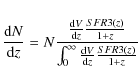
The results presented in the last section rely on the validity of the duration-luminosity relation (DLR) for pulses. If confirmed, the DLR would also offer a new method to estimate GRB distances, simpler and easier to use than the LLR (Hakkila et al. 2009). Bursts with several pulses give the possibility of multiple measures of the redshift, increasing the resulting accuracy. Conversely the identical redshift for all pulses in a given burst allows to test the DLR. Assuming a power-law of the form $L\propto t_{\rm p}^{-s}$ Hakkila et al. (2009) find $s=0.8 \pm 0.4$ for a sample of 53 multi-pulsed GRBs, which is consistent with the result obtained from bursts with known redshift.

We have performed an alternative and independent test of the DLR using a synthetic population of GRB pulses for which we predict the resulting observational duration-peak photon flux ( $t_{\rm p}^{\rm obs}$ - P) diagram which is then compared to real data. The synthetic population is generated following a Monte-Carlo method similar to the one described in Daigne et al. (2006): for each pulse we draw a redshift z and a peak luminosity L. We then either link $E_{\rm p}$ and $t_{\rm p}$ to the luminosity with Eqs. (7) and (8) or adopt log-normal distributions independent of L. We want to see if the predicted $t_{\rm p}^{\rm obs}$ - P diagram is in better agreement with the data when the DLR is adopted.

Even if $t_{\rm p}$ and L are uncorrelated we expect a first trend purely due to cosmological effects as more distant pulses are globally weaker and have longer durations. If an intrinsic relation such as Eq. (8) is also satisfied the trend should be more pronounced. The analysis by Hakkila & Cumbee (2009) of a sample of pulses extracted from 106 long GRBs gives $P\propto t_{\rm p}^{-0.27}$ which is shallower than Eq. (8). The observed population is however affected by cosmological effects (time dilation and k-correction) on the pulse duration (Norris 2002) and by selection effects due to instrument threshold. We model these different effects to generate the simulated observational $t_{\rm p}^{\rm obs}$ - P diagram from our synthetic GRB pulse population.

3.2 The synthetic pulse population

To get the distribution of the pulse parameters z, L, $E_{\rm p}$ and $t_{\rm p}$ in the synthetic sample we make the following assumptions:

-

redshift z: as we only consider long GRBs which have massive progenitors, the GRB rate $R_{\rm GRB}(z)$ could a priori be expected to be proportional to the cosmic star formation rate ${\it SFR}(z)$ . However recent studies (Daigne et al. 2006; Guetta & Piran 2007; Kistler et al. 2008) have shown that at large z the GRB rate still increases while the SFR probably decreases or remains constant. This suggests that stellar populations at large z are more efficient in producing GRBs for reasons which are not well understood (reduced metallicity or/and IMF favoring massive stars). In this study we adopt a burst rate which follows SFR3 of Porciani & Madau (2001). This SFR which keeps rising at large z is not realistic as it would overproduce metals at early cosmic times but $R_{\rm GRB}$ $\propto$ SFR3(z) provides a good fit of the redshift distribution of Swift bursts. We then generate a table of N (N from 10³ to 10⁶) values of the redshift and corresponding luminosity distance $d_{\rm L}(z)$ with z being distributed as

$\begin{displaymath}{{\rm d}N\over {\rm d}z}=N{{{\rm d}V\over {\rm d}z} {SFR3(z)\... ...r \int_0^{\infty}{{\rm d}V\over {\rm d}z} {SFR3(z)\over 1+z}} \end{displaymath}$

(9)

where ${\rm d}V\over {\rm d}z$ is the comoving volume element in the concordance cosmology;

-

luminosity L: we adopt a power law luminosity function $\Phi(L)\propto L^{-\delta}$ between $L_{\rm min}$ and $L_{\rm max}$ . For the burst population it has been shown that a power law LF with $1.5<\delta<2$ can reproduce the ${\rm Log}~N$ - ${\rm Log}~P$ curve (Firmani et al. 2004; Daigne et al. 2006). We adopt the same range of values here and vary $L_{\rm min}$ and $L_{\rm max}$ respectively from 10⁵⁰ to 10⁵¹ erg s^-1 and from 10⁵³ to 10⁵⁴ erg s^-1;

-

spectral parameters: the peak energy is either obtained from the luminosity with the Amati-like relation or has a log-normal distribution of central value $E_{{\rm p},0}$ and width $\sigma_0$ . When the Amati-like relation is adopted we add a dispersion $\sigma_{\rm A}$ around Eq. (7). We draw the spectral indices $\alpha$ and $\beta$ in agreement with the distributions found by Preece et al. (2000) for bright BATSE bursts. In Daigne et al. (2006) the values of $\sigma_0$ , $E_{{\rm p},0}$ and $\sigma_{\rm A}$ were adjusted to provide a good fit of the $E_{\rm p}$ distribution of bright BATSE bursts. We keep the same values as a starting point but we also vary them since we are now considering individual pulses rather than the entire bursts;

-

duration: to get the pulse duration we either assume the validity of the DLR (Eq. (8)) with a dispersion $\sigma_{\rm t_{\rm p}}$ or adopt a log-normal distribution of central value and dispersion adjusted to reproduce the observed distribution of pulse duration in the Hakkila & Cumbee (2009) sample.

For a given pulse, the observable quantities P and $t_{\rm p}^{\rm obs}$ are then computed from the intrinsic parameters. For the peak photon flux we have, assuming a normalized Band spectrum (i.e. $\int_0^{\infty}{\cal B}(x)=1$ )

$\begin{displaymath}P={L\over 4\pi~d_{\rm L}^2~E_{\rm p}^{\rm obs}}\int_{50/E_{\rm p}^{\rm obs}} ^{300/E_{\rm p}^{\rm obs}}{\cal B}(x){\rm d}x \end{displaymath}$

(10)

where $E_{\rm p}^{\rm obs}=E_{\rm p}/(1+z)$ . To obtain the observed pulse duration we take into account both time dilation and the approximate dependence of pulse width with energy $t_{\rm p}\propto E^{-0.4}$ (Norris et al. 1996) so that

$\begin{displaymath}t_{\rm p}^{\rm obs}\simeq (1+z)^{0.6}~t_{\rm p} . \end{displaymath}$

(11)

We adopt the threshold prescription from Band (2003) where the limiting photon flux is defined between 1 and 1000 keV and depends on the observed peak energy. This finally allows us to construct the simulated observational $t_{\rm p}^{\rm obs}$ - P diagram for comparison to real data.

3.3 Results

We define a reference case which corresponds to the following choice of the parameters: slope of the luminosity function $\delta=1.7$ ; $L_{\rm min}=10^{51}$ erg s^-1; peak energy obtained from the Amati-like relation (Eq. (7)) with an added dispersion of 0.3 dex. We compare in Fig. 5 the resulting $t_{\rm p}^{\rm obs}$ - P diagrams with and without the DLR. When the DLR is adopted we again assume a dispersion of 0.3 dex around Eq. (8). A fit of the diagrams by a power-law $P\propto t_{\rm p}^{-s}$ respectively gives s=0.27 (with the DLR) and s=0.09 (without). In the first case, the agreement with the data of Hakkila & Cumbee (2009) is excellent while the correlation almost disappears in the second case.

$\begin{figure} \par\resizebox{19cm}{!}{\includegraphics{14132f5a.eps} \includegraphics{14132f5b.eps}} \vspace*{4mm} \end{figure}$	Figure 5: $t_{\rm p}^{\rm obs}$ - P diagram for a sample of 750 synthetic pulses corresponding to our reference case (see text for details). The left panel, which assumes the validity of the DLR looks very similar to the data collected by Hakkila & Cumbee (2009). The right panel, with a log-normal distribution of pulse duration do not show a significant correlation between the two quantities.
Open with DEXTER

We then checked how these results are changed when we vary the model parameters and assumptions (see Table 1):

Table 1: Slope s of a power law fit ( $P\propto t_{\rm p}^{-s}$ ) of the $t_{\rm p}$ - P diagram with and without the assumption of the DLR (Eq. (8)) for pulses.

-: Luminosity function: we list the power-law index s of the $t_{\rm p}^{\rm obs}$ - P relation when we vary the lower and upper limits of the luminosity function $L_{\rm min}$ and $L_{\rm max}$ and its slope $\delta$ . It can be seen that the results only weakly depend on $L_{\rm min}$ and $L_{\rm max}$ and are nearly unsensitive to $\delta$ .
-: Peak energy distribution: we have first replaced the Amati relation by a log-normal distribution of central value $E_{\rm p}=600$ keV and dispersion 0.3 dex which were the values adopted by Daigne et al. (2006). Since these corresponded to the whole burst spectra and not to individual pulses we have considered other possible $E_{\rm p}$ values. We find that the power-law index of the $t_{\rm p}^{\rm obs}$ - P relation is practically independent of the adopted $E_{\rm p}$ , especially when we assume the validity of DLR. However in this case the $t_{\rm p}^{\rm obs}$ - P relation becomes somewhat steeper than the data (with s=0.33).
-: Dispersion of the DLR: we have increased the dispersion of the DLR from $\sigma_{\rm t_{\rm p}}=0.3$ dex to 1.5 dex. We observe that the power-law index of the $t_{\rm p}^{\rm obs}$ - P relation evolves from its reference value of 0.27 to 0.09 which corresponds to the situation without the DLR. It appears that the dispersion of the DLR cannot exceed about 0.6 dex if we still want to fit the data.

Our study then indicates that an intrinsic correlation between pulse duration and luminosity is necessary to reproduce the observed $t_{\rm p}^{\rm obs}$ - Pdiagram. This conclusion is not affected when we vary the model paramaters such as the luminosity function or the spectral properties of pulses. It is also robust regarding changes in the adopted sensitivity: when we decrease (resp. increase) the threshold by a factor of two, the $t_{\rm p}^{\rm obs}$ - Pcorrelation becomes only slightly steeper (resp. shallower).

Nevertheless, a few words of caution should be expressed since our analysis does not take into account possible additional selection effects which may not apply equally to pulses of different durations. For example the data has been collected with a trigger criterion applied to the full burst and not to individual pulses. It therefore includes some pulses below the threshold, coming from bursts which triggered at a brighter instant of the light curve. Also, the pulse selection and identification technique can fail when many pulses overlap, which is another source of selection effects, not easy to quantify. It is possible that these different biases contribute to produce an effective threshold with a limit in fluence in addition to the adopted limit in peak flux. A limit in fluence may artificially generate a trend in the P - $t_{\rm p}^{\rm obs}$ diagram which could contribute to the observed relation.

4 Discussion

Assuming the validity of the duration-luminosity relation, we have tried to see if it can be understood in the context of the internal shock model for the prompt emission of GRBs (Rees & Meszaros 1994). The isotropic luminosity generated by internal shocks can be approximated by

$\begin{displaymath}L=\dot E~ f(\kappa)~ \epsilon_{\rm e} \end{displaymath}$

(12)

where $\dot E$ is the isotropic kinetic power in the relativistic flow, $f(\kappa)$ is the efficiency of dissipation by internal shocks (which mainly depends on the contrast $\kappa$ between the maximum and minimum Lorentz factors) and $\epsilon_{\rm e}$ is the fraction of the dissipated energy which is transferred to electrons and eventually radiated.

It can be seen that the time scale $\tau$ for variability of the Lorentz factor does not explicitely appear in Eq. (12). As the observed variability of the prompt emission reflects that of the Lorentz factor in the internal shock model (times the (1+z) dilation) any duration-luminosity relation implies that $\tau$ should be in some way linked to $\dot E$ and possibly also to $\kappa$ or $\epsilon_{\rm e}$ . One could for example imagine that increasing $\dot E$ results in a more unstable outflow where the Lorentz factor fluctuates on a shorter time scale. This would induce a DLR which could become even more pronounced if the amplitude of the fluctuations (and therefore $\kappa$ ) also increases with $\dot E$ .

From an observational point of view there are some indications that $\dot E$ is anticorrelated with the opening angle of the relativistic jet (Frail et al. 2001). A thinner jet drilling its way through the envelope of the progenitor star could be more sensitive to Kelvin-Helmholtz instabilities developing at its boundaries (Aloy et al. 2002). This would lead to a more irregular outflow with a shorter time scale of variability of the Lorentz factor, finally leading to a DLR. But clearly this discussion is somewhat speculative and it remains that the internal shock model does not provide by itself a simple and direct way to explain the DLR.

Recently the internal shock model has also been criticized for a series of reasons such as its low efficiency, the difficulty to explain the standard value $\alpha \sim -1$ of the low energy index of the spectrum (Ghisellini et al. 2000) or the possible complete suppression of shocks if the flow is strongly magnetized. Proposed alternatives to internal shocks are reconnection processes (Giannos & Spruit 2007) relativistic turbulence (Narayan & Kumar 2009; Lazar et al. 2009) or comptonized photospheric emission (Beloborodov 2009). Unfortunately the modelling of these mechanisms has not reached a degree of accuracy where detailed predictions can be made on the properties of pulses.

5 Conclusion

We have considered the relations existing between spectral lags, duration and luminosity in GRB pulses. Extending a previous work by Hafizi & Mochkovitch (2007) we have first shown that the lag over pulse duration ratio does not vary much among pulses (remaining of the order of a few percents). This result holds as long as the spectral softening following pulse maximum is not limited to a decrease of the peak energy but also affects the spectral indices, as indicated by the observations. We have then included in our analysis the relation between pulse duration and luminosity recently discovered by Hakkila et al. (2008). Combined to our results it allows to link all three quantities: $\Delta t$ , $t_{\rm p}$ and L. The lag-duration and lag-luminosity relations we obtain are in good agreement with the data. Also, they do not strongly depend on the assumptions for the spectral parameters at pulse maximum: values of $E_{\rm p}$ , $\alpha$ , $\beta$ and their derivatives, Amati relation or log-normal distribution of $E_{\rm p}$ .

Originally obtained with a limited set of only 12 pulses the DLR has recently received further support from the analysis of another sample of 12 pulses coming from 8 bursts detected by the HETE 2 satellite (Arimoto et al. 2010). Its validity however still needs to be confirmed and we have therefore proposed to test it in a different (statistical) way using the observational duration-peak photon flux ( $t_{\rm p}^{\rm obs}$ - P) diagram. For that purpose, we have adapted the Monte-Carlo code of Rossi et al. (2006) to generate a sample of synthetic pulses for which we predict the observational $t_{\rm p}^{\rm obs}$ - P diagram. It appears that the observed correlation $P\propto t_{\rm p}^{-0.27}$ is reproduced only if pulses satisfy the DLR. This conclusion remains valid when we vary the pulse luminosity function and spectral properties ( $E_{\rm p}$ obtained from the Amati relation or having a log-normal distribution). Nevertheless we cannot completely exclude some bias in the pulse selection and characterization process which could contribute to the observed relation even in the absence of a DLR.

We have finally confronted the DLR to the prediction of the internal shock model for the prompt emission. It appears that the DLR cannot be obtained as a direct and simple consequence of the model. Additional assumptions are required, for example the possibility that the relativistic outflow becomes more unstable and variable when the injected kinetic power increases. Proposed alternatives to internal shocks - reconnection, relativistic turbulence, comptonized photosphere - still don't have the predictive power to test if they can explain the DLR.

In a future development of this work we plan to extend our analysis of the pulse properties (width and spectral lags) to other energy ranges. Data are sparse in the optical but the detailed light curve of the ``naked-eye burst'' GRB 080319b has for example revealed interesting correlations between spectral lags at high and low energy (Stamatikos et al. 2009). At very high energy, Fermi observations have shown delays in the onset of the LAT component with respect to the MeV emission. Understanding the origin of these behaviors will provide clues for a better understanding of the prompt emission of GRBs.

Acknowledgements

It is a pleasure to thank Jon Hakkila for his numerous advices and for having sent to us unpublished materials and data. We also thank Makoto Arimoto who has kindly answered our questions about the HETE 2 data.

References

Aloy, M. A., Ibañez, J. M., Miralles, J. A., & Urpin, V. 2002, A&A, 396, 693
Amati, L., Frontera, F., Tavani, M., et al. 2002, A&A, 390, 81
Arimoto, M., Kawai, N., Asano, K., et al. 2010, PASJ, 62, 487
Band, D. 2003, ApJ, 588, 945
Band, D., Matteson, J., Ford, L., et al. 1993, ApJ, 413, 281
Beloborodov, A. M. 2009, MNRAS, 407, 1033
Daigne, F., Rossi, E. M., & Mochkovitch, R. 2006, MNRAS, 372, 1034
Firmani, C., Avila-Reese, V., Ghisellini, G., & Tutukov, A. V. 2004, ApJ, 611, 1033
Frail, D. A., Kulkarni, S. R., Sari, R., et al. 2001, ApJ, 562, L55
Gehrels, N., Norris, J. P., Mangano, V., et al. 2006, Nature, 444, 1044
Ghirlanda, G., Ghisellini, G., Lazzati, D., & Firmani, C. 2004, ApJ, 613, L13
Ghirlanda, G., Ghisellini, G., Firmani, C., et al. 2005, MNRAS, 360, L45
Ghisellini, G., Celotti, A., & Lazzati, D. 2000, MNRAS, 313, L1
Giannos, D., & Spruit, H. C. 2007, A&A, 469, 1
Golenetskii, S. V., Mazets, E. P., Aptekar, R. L., & Ilinskii, V. N. 1983, Nature, 306, 451
Guetta, D., & Piran, T. 2007, JCAP, 7, 3
Hafizi, M., & Mochkovitch, R. 2007, A&A, 465, 67
Hakkila, J., & Cumbee, R. S. 2009, in Sixth Huntsville Gamma-Ray Burst Conf., ed. C. A. Meegan, & N. Gehrels, & C. Kouveliotou, AIP Conf. Proc., 1133, 379
Hakkila, J., Giblin, T. W., Young, K. C., et al. 2007, ApJS, 169, 62
Hakkila, J., Giblin, T. W., Norris, J. P., et al. 2008, ApJ, 677, L81
Hakkila, J., Fragile, P. C., & Giblin, T. W. 2009, in Sixth Huntsville Gamma-Ray Burst Conf., ed. C. A. Meegan, N. Gehrels, & C. Kouveliotou, AIP Conf. Proc., 1133, 479
Kistler, M. D., Yüksel, H., Beacom, J. F., & Stanek, K. Z. 2008, ApJ, 673, L119
Kouveliotou, C., Meegan, C. A., Fishman, G. J., et al. 1993, ApJ, 413, L101
Lazar, A., Nakar, E., & Piran, T. 2009, ApJ, 695, L10
Liang, E., & Kargatis, V. 1996, Nature, 381, 49
Narayan, R., & Kumar, P. 2009, MNRAS, 394, L117
Norris, J. P. 2002, ApJ, 579, 386
Norris, J. P., & Bonnell, J. T. 2006, ApJ, 643, 266
Norris, J. P., Nemiroff, R. J., Bonnell, J. T., et al. 1996, ApJ, 459, 393
Norris, J. P., Marani, G. F., & Bonnell, J. T. 2000, ApJ, 534, 248
Porciani, C., & Madau, P. 2001, ApJ, 548, 522
Preece, R. D., Briggs, M. S., Mallozzi, R. S., et al. 2000, ApJS, 126, 19
Reichart, D. E., Lamb, D. Q., Fenimore, E. E., et al. 2001, ApJ, 552, 57
Stamatikos, M., Ukwatta, T. N., Sakamoto, T., et al. 2009, in Sixth Huntsville Gamma-Ray Burst Conf., ed. C. A. Meegan, N. Gehrels, & C. Kouveliotou, AIP Conf. Proc., 1133, 356

All Tables

Table 1: Slope s of a power law fit ( $P\propto t_{\rm p}^{-s}$ ) of the $t_{\rm p}$ - P diagram with and without the assumption of the DLR (Eq. (8)) for pulses.

All Figures

$\begin{figure} \par\includegraphics[width=10.4cm,clip]{14132f1.eps} \end{figure}$	Figure 1: Plot of the three functions $f_{13,E_{\rm p}}$ (full line), $-f_{13,\alpha }$ (dotted line) and $-f_{13,\beta }$ (dashed line) for $\alpha =-1$ and $\beta =-2.25$ .
Open with DEXTER
In the text

$\begin{figure} \par\includegraphics[width=10.4cm,clip]{14132f2.eps} \end{figure}$	Figure 2: Ratio of spectral lag over pulse duration as a function of the peak energy at pulse maximum (lower scale) and of the peak luminosity (upper scale) assuming the validity of the Amati-like relation (Eq. (7)). The full lines correspond to ${\dot e}_{\rm p}=-0.5$ and from top to bottom respectively to $\dot a=\dot b=0.2$ , 0.1 and 0. The dashed lines have the same $\dot a$ and $\dot b$ but ${\dot e}_{\rm p}=-0.25$ . The adopted value of the curvature parameter is \|C₁\|=10.
Open with DEXTER
In the text

$\begin{figure} \par\includegraphics[width=10.4cm,clip]{14132f3.eps} \end{figure}$	Figure 3: Plot of the pulse duration as a function of spectral lag. The full thick line represents our reference model which adopts the Amati-like relation (Eq. (7)) and $\alpha =-1$ , $\beta =-2.25$ , $\dot E=-0.5$ , $\dot a=\dot b=0.1$ and \|C₁\|=10. The thin lines correspond to nine other cases with different choices of the parameters (see text for details). The squares are the data points of the sample considered in Hakkila et al. (2008).
Open with DEXTER
In the text

$\begin{figure} \par\includegraphics[width=10.4cm,clip]{14132f4.eps} \end{figure}$	Figure 4: Theoretical lag-luminosity relation for pulses compared to the data collected by Hakkila et al. (2008). The thick line is the reference case while the thin lines correspond to different model parameters (see Fig. 3 and text for details).
Open with DEXTER
In the text

$\begin{figure} \par\resizebox{19cm}{!}{\includegraphics{14132f5a.eps} \includegraphics{14132f5b.eps}} \vspace*{4mm} \end{figure}$	Figure 5: $t_{\rm p}^{\rm obs}$ - P diagram for a sample of 750 synthetic pulses corresponding to our reference case (see text for details). The left panel, which assumes the validity of the DLR looks very similar to the data collected by Hakkila & Cumbee (2009). The right panel, with a log-normal distribution of pulse duration do not show a significant correlation between the two quantities.
Open with DEXTER
In the text

Current usage metrics show cumulative count of Article Views (full-text article views including HTML views, PDF and ePub downloads, according to the available data) and Abstracts Views on Vision4Press platform.

Data correspond to usage on the plateform after 2015. The current usage metrics is available 48-96 hours after online publication and is updated daily on week days.

Initial download of the metrics may take a while.