| Issue |
A&A
Volume 519, September 2010
|
|
|---|---|---|
| Article Number | A90 | |
| Number of page(s) | 19 | |
| Section | Cosmology (including clusters of galaxies) | |
| DOI | https://doi.org/10.1051/0004-6361/201014098 | |
| Published online | 16 September 2010 | |
Strong lensing in the MARENOSTRUM UNIVERSE
I. Biases in the cluster lens population
M. Meneghetti1,3 - C. Fedeli2,3 - F. Pace4 - S. Gottlöber5 - G. Yepes6
1 - INAF - Osservatorio Astronomico di Bologna, via Ranzani 1, 40127 Bologna, Italy
2 - Dipartimento di Astronomia, Università di Bologna, via Ranzani 1, 40127 Bologna, Italy
3 - INFN, Sezione di Bologna, Viale Berti Pichat 6/2, 40127 Bologna, Italy
4 - ITA, Zentrum für Astronomie, Universität Heidelberg, Albert Überle Str. 2, 69120 Heidelberg, Germany
5 - Astrophysikalisches Institut Potsdam, An der Sternwarte 16, 14482 Potsdam, Germany
6 - Grupo de Astrofísica, Universidad Autónoma de Madrid, 28049 Madrid, Spain
Received 19 January 2010 / Accepted 18 March 2010
Abstract
Context. Strong lensing is one of the most direct probes of
mass distribution in the inner regions of galaxy clusters. It can be
used to constrain the density profiles and to measure the mass of the
lenses. Moreover, the abundance of strong lensing events can be used to
constrain structure formation and cosmological parameters through the
so-called ``arc-statistics'' approach. However, several issues related
to the use of strong lensing clusters in cosmological applications are
still controversial, leading to the suspicion that several biases may
affect this very peculiar class of objects.
Aims. With this study we aim a better understanding of the properties of galaxy clusters that can potentially act as strong lenses.
Methods. We do so by investigating the properties of a large sample of galaxy clusters extracted from the N-body/hydrodynamical simulation M AREN OSTRUM U NIVERSE.
We perform ray-tracing simulations with each of them and identify those
objects capable of producing strong lensing effects. We explore the
correlation between the cross section for lensing and many properties
of clusters, such as mass, three-dimensional and projected shapes,
their concentrations, the X-ray luminosity, and the dynamical activity.
Results. We quantify the minimal cluster mass required for
producing both multiple images and large distortions. While we do not
measure a significant excess of triaxiality in strong lensing clusters,
we find that the probability of strong alignments between the major
axes of the lenses and the line of sight is a growing function of the
lensing cross section. In projection, the strong lenses appear rounder
within R200, but we find that their cores tend to be
more elliptical as the lensing cross section increases. As a result of
the orientation bias, we also find that the cluster concentrations
estimated from the projected density profiles tend to be biased high.
The X-ray luminosity of strong lensing clusters tend to be higher than
for normal lenses of similar mass and redshift. This is particularly
significant for the least massive lenses. Finally, we find that the
strongest lenses generally exhibit an excess of kinetic energy within
the virial radius, thus indicating that they are more dynamically
active than the usual clusters.
Conclusions. We conclude that strong lensing clusters are a very
peculiar class of objects, affected by many selection biases that need
to be properly modeled when using them to study the inner structure of
galaxy clusters or to constrain the cosmological parameters.
Key words: gravitational lensing: strong - galaxies: clusters: general
1 Introduction
Gravitational lensing is one of the most powerful tools available for studying the formation of cosmic structures in the universe. The light from distant sources, traveling in space and time, is deflected by matter along its path before being collected by observers. Thus, we measure an integrated effect that contains a wealth of information about the cosmic structures at different epochs.
Depending on the impact parameter on the intervening matter and on the mass of the deflectors encountered by the light along its path, gravitational lensing manifests itself in weak and strong regimes. In the weak-lensing regime the shapes of distant galaxies, which happen to be at large angular distances from the highest mass concentrations on the sky, are slightly changed, such that this effect can only be revealed though statistical measurements. Nevertheless, these tiny distortions can be used for tracing the large-scale structure of the universe both in two and in three dimensions (see e.g. Massey et al. 2007; Benjamin et al. 2007; Fu et al. 2008, for some recent results), from which important cosmological constraints can be derived (Bartelmann & Schneider 2001). This is a field of research that will extraordinarily improve in the next decades thanks to some upcoming missions (Kaiser 2007; Wittman et al. 2006; Refregier et al. 2008; Jelinsky & SNAP Collaboration 2006). Weak lensing allows reconstruction of the mass distribution up to the outskirts of galaxy clusters (see e.g. Hoekstra 2007; Dahle 2006; Clowe et al. 2006).
Strong lensing is a highly nonlinear and relatively rare effect that is observable in the central regions of galaxies and clusters. In this regime, the background sources can be imaged many times over and/or highly distorted to form very elongated images, the so-called ``gravitational arcs''. They are powerful cosmological probes for many reasons. First, such events can be used to investigate the inner regions of the lenses. Thus, they can be used to test the predictions of the cold-dark-matter paradigm on the inner structure of dark matter halos (Mao et al. 2004; Bartelmann & Meneghetti 2004; Sand et al. 2004; Limousin et al. 2008; Meneghetti et al. 2007b,2001). Second, they can be used to recover the mass distribution in the center of the lenses, providing complementary informations to those obtained from weak lensing (Cacciato et al. 2006; Limousin et al. 2007; Merten et al. 2009; Bradac et al. 2005; Diego et al. 2005). Lensing masses can then be used for measuring the cluster mass function. Third, the position and the distortions of the strongly lensed images as a function of the source redshift reflect the geometry of the universe (Soucail et al. 2004; Meneghetti et al. 2005b). Finally, the probability of observing strong lensing events is deeply connected to the abundance, the mass, and the formation epoch (through the concentration) of the lenses. This makes statistical lensing a potentially powerful tool for studying the structure formation (Meneghetti et al. 2005a; Bartelmann et al. 1998; Li et al. 2005).
In this paper, we focus on the properties of the most massive and
therefore most efficient strong lenses in the universe: the galaxy
clusters. In the framework of the hierarchical scenario of structure
formation, these are the youngest bound systems in the sky. About ![]() of their mass is believed to be in the form of cold dark matter (Gottlöber & Yepes 2007). The remaining
of their mass is believed to be in the form of cold dark matter (Gottlöber & Yepes 2007). The remaining ![]() is made of a diffuse gas component, the intra-cluster-medium, and of
other baryons in the form of stars, the vast majority of which are
inside the cluster galaxies. Because they are relatively young
structures, the interaction between the baryons and the dark matter is
weaker than in older systems like galaxies. For this reason, clusters
are important laboratories for studying the properties of the dark
matter (Markevitch et al. 2004).
However, there are several issues that we need to consider when
studying these systems. In particular, clusters where gravitational
arcs are observed are a limited fraction of the total number (Sand et al. 2005; Gladders et al. 2003; Hennawi et al. 2008; Luppino et al. 1999; Zaritsky & Gonzalez 2003) and therefore a particular class of objects.
is made of a diffuse gas component, the intra-cluster-medium, and of
other baryons in the form of stars, the vast majority of which are
inside the cluster galaxies. Because they are relatively young
structures, the interaction between the baryons and the dark matter is
weaker than in older systems like galaxies. For this reason, clusters
are important laboratories for studying the properties of the dark
matter (Markevitch et al. 2004).
However, there are several issues that we need to consider when
studying these systems. In particular, clusters where gravitational
arcs are observed are a limited fraction of the total number (Sand et al. 2005; Gladders et al. 2003; Hennawi et al. 2008; Luppino et al. 1999; Zaritsky & Gonzalez 2003) and therefore a particular class of objects.
Broadly speaking they are the most massive clusters, but there are
several other properties that boost the cluster ability to produce
strong lensing events. For example, we know that substructures,
asymmetries, and projected ellipticity of the lenses all contribute to
the strong lensing cross section of clusters (Meneghetti et al. 2003b, 2007a). Both observations and simulations agree that strong lenses have high concentrations (Fedeli et al. 2007a; Broadhurst et al. 2008; Kneib et al. 2003; Gavazzi et al. 2003; Hennawi et al. 2007). Triaxiality is also relevant, because clusters seen along their major axis are more efficient lenses (Oguri et al. 2003). Although cluster galaxies statistically do not change the distributions of the arc properties (Meneghetti et al. 2000; Hilbert et al. 2008; Flores et al. 2000), cD galaxies sitting at the bottom of the cluster potential well increase the ability to produce long and thin arcs by ![]() 30-50% (Meneghetti et al. 2003a). The gas physics, in particular cooling, could also affect the strong lensing properties of clusters (Puchwein et al. 2005; Mead et al. 2010; Wambsganss et al. 2008). Finally, Torri et al. (2004)
show that the cluster ability to produce gravitational arcs can also be
enhanced by the dynamical activity in the lens. By studying with high
time resolution how the lensing cross section changes during an edge-on
collision between the main cluster clump and a substructure, these
authors find that the strong lensing efficiency is boosted by a factor
of 10 during the merging phase. Later, Fedeli et al. (2006)
used semi-analytic methods to show that the arc optical depth produced
by clusters with moderate and high redshifts is more than doubled by
mergers.
30-50% (Meneghetti et al. 2003a). The gas physics, in particular cooling, could also affect the strong lensing properties of clusters (Puchwein et al. 2005; Mead et al. 2010; Wambsganss et al. 2008). Finally, Torri et al. (2004)
show that the cluster ability to produce gravitational arcs can also be
enhanced by the dynamical activity in the lens. By studying with high
time resolution how the lensing cross section changes during an edge-on
collision between the main cluster clump and a substructure, these
authors find that the strong lensing efficiency is boosted by a factor
of 10 during the merging phase. Later, Fedeli et al. (2006)
used semi-analytic methods to show that the arc optical depth produced
by clusters with moderate and high redshifts is more than doubled by
mergers.
Although extensive work has been done in the past decade, a better characterization of the strong lens cluster population is mandatory. Given the complexity of clusters and the importance that many of their properties have for strong lensing, the only reliable way to do that is through ray-tracing analysis of a large number of simulated clusters. A first important work in this framework was done by Hennawi et al. (2007), who analyzed a sample of 878 clusters from an N-Body pure dark-matter cosmological simulation. Important properties like concentrations, axis ratios, and substructures are discussed there. In this work, we aim to extend the analysis of Hennawi et al. (2007) in three ways. First, we include a much larger number of clusters (now 49 366 systems), taken from a larger cosmological volume ( 500 h-1 Mpc vs. 320 h-1 Mpc). Second, the clusters used here were obtained from an N-body-hydrodynamical simulation where the evolution of the gas component is also considered. Thus, we can correlate the lensing properties of clusters with some important X-ray observables. Third, we study in detail the possible correlations between cluster dynamics and strong lensing efficiency, which has so far been made only through analytical models.
The plan of the paper is as follows. In Sect. 2 we summarize the main characteristics of the cosmological simulation M AREN OSTRUM U NIVERSE. In Sect. 3 we discuss the simulation methods and define several lensing quantities useful for the following analysis. In Sect. 4 we discuss the correlation between lens masses and strong lensing ability. Section 5 is dedicated to the statistical analysis of the shapes and orientations of strong lensing clusters. We discuss the biases in the concentrations in Sect. 6. In Sect. 7 we focus on the X-ray properties of strong lensing clusters. Finally, in Sect. 8 we correlate the strong lensing efficiency with the dynamical state of the lenses, and summarize the main results and the conclusions of this study in Sect. 9.
2 The MARENOSTRUM UNIVERSE simulation
The M AREN OSTRUM U NIVERSE (Gottlöber & Yepes 2007) is a large-scale cosmological non-radiative SPH simulation performed with the G ADGET2 code (Springel 2005). We briefly summarize the relevant characteristics here, and refer the reader to the paper by Gottlöber & Yepes (2007) for a more detailed description of the simulation. This was run in 2005, during the testing period of the MareNostrum supercomputer using the WMAP1 normalisation, namelyTo find all structures and substructures within the distribution of 2 billion particles and to determine their properties, we use a hierarchical friends-of-friends (FOF) algorithm (Klypin et al. 1999). With a basic linking length set to 0.17 times the mean interparticle distance, we extract the FOF objects at all redshifts. The final catalog of identified objects contains more than 2 million objects with more than 20 DM particles at z=0. The same objects and their progenitors are contained in the catalogs corresponding to higher redshift outputs of the simulation. In this sense a correlation exists between different redshift slices. In a second step we divide the linking length by 2n (n=1,3) to find substructures of the clusters. In particular, we use n=2 to identify the highest density peak that we associate with the center of the cluster.
All the FOF groups with mass larger than
![]() are then stored into sub-boxes of cubic shape with side length
are then stored into sub-boxes of cubic shape with side length ![]() Mpc for the subsequent lensing analysis.
Mpc for the subsequent lensing analysis.
3 Lensing properties
3.1 Ray-tracing
In this section, we illustrate the techniques used to derive the strong lensing properties of the clusters in the M AREN OSTRUM U NIVERSE cosmological volume.
The deflection angle maps are calculated as explained in several previous papers (see e.g. Meneghetti et al. 2005a,2000). The particles in each cube are used to produce a 3D density field, by interpolating their
position on a grid of 5123 cells using the Triangular Shaped
Cloud method (Hockney & Eastwood 1988). Then, we project the 3D
density field along the coordinate axes, obtaining three surface
density maps
![]() ,
used as lens planes in the following
lensing simulations.
,
used as lens planes in the following
lensing simulations.
The next step consists of tracing bundles of light rays through a
regular grid covering the central part of each lens plane. We choose to
set the size of this region as
![]() Mpc2
comoving. This choice is driven by the necessity to
study in detail the central region of the clusters, where critical
curves form. However, we do this by considering the contribution from
the surrounding mass distribution to the deflection angle of each ray.
Mpc2
comoving. This choice is driven by the necessity to
study in detail the central region of the clusters, where critical
curves form. However, we do this by considering the contribution from
the surrounding mass distribution to the deflection angle of each ray.
We first define a grid of
![]() ``test'' rays, and the deflection angle for each is calculated by
directly summing the contributions from all cells on the surface
density map
``test'' rays, and the deflection angle for each is calculated by
directly summing the contributions from all cells on the surface
density map
![]() ,
,
|
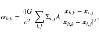
(1) |
where A is the area of one pixel on the surface density map, and
3.2 Strong lensing clusters
For a fixed-source redshift, a cluster can produce strong lensing events if it develops critical lines on the lens plane. These lines correspond to the caustics on the source plane. Only sources within the caustics have multiple images, and only sources that happen to lie close to the caustics are strongly distorted and magnified.
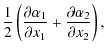
A cluster can produce both tangential and radial critical
lines, where the tangential and the radial magnifications diverge,
respectively. The critical lines form where
| (2) |
where
| |
= | 
|
(3) |
| = | 
|
(4) | |
| = | 
|
(5) |
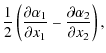
It can be shown that the convergence is the surface density divided by a critical surface density:
| (6) |
which depends on the angular diameter distances between observer and lens,
|
(7) |
It is clear that, in order to be a strong lens, the cluster convergence and shear must be large enough, such that their sum is larger than unity somewhere.
To focus on the subsample of strong lenses, we start by selecting
those halos that are capable of developing critical lines. For doing
this, we use the
![]() test rays first. We numerically calculate the spatial derivatives of the deflection angles to compute
test rays first. We numerically calculate the spatial derivatives of the deflection angles to compute ![]() and
and ![]() and to determine the positions of the critical points. If at least a
critical point is found in the three cluster projections using these
maps, we consider the cluster for further, more detailed analysis. We
are aware that, by using this selection criterium, all lenses whose
critical lines have sizes smaller than
and to determine the positions of the critical points. If at least a
critical point is found in the three cluster projections using these
maps, we consider the cluster for further, more detailed analysis. We
are aware that, by using this selection criterium, all lenses whose
critical lines have sizes smaller than ![]() 20 h-1 kpc
comoving, corresponding to the spatial resolution of the coarse grid,
are not included in our analysis. Because of these limitations, our
results should be used with caution in referring to small strong
lensing systems. Instead, such objects would never produce significant
image splittings and large distortions, or giant arcs, which are the
most relevant strong lensing features in this work.
20 h-1 kpc
comoving, corresponding to the spatial resolution of the coarse grid,
are not included in our analysis. Because of these limitations, our
results should be used with caution in referring to small strong
lensing systems. Instead, such objects would never produce significant
image splittings and large distortions, or giant arcs, which are the
most relevant strong lensing features in this work.
As a result of this preliminary selection, it turns out that
49 366 clusters produce critical curves for sources at
redshift
![]() in at least one of their projections. For these objects, we repeat the
calculation of the deflection angles on grids with higher spatial
resolution on all three projections, obtaining
148 098 deflection angle maps.
in at least one of their projections. For these objects, we repeat the
calculation of the deflection angles on grids with higher spatial
resolution on all three projections, obtaining
148 098 deflection angle maps.
3.3 Cross-sections for giant arcs
Once the high-resolution deflection angle maps for the three
projections of each numerical cluster are computed, the strong lensing
efficiency for long and thin arcs was evaluated by using the fast,
semi-analytic algorithm presented in Fedeli et al. (2006).
The reader is referred to the quoted paper for details, while here we
just give a quick overview of the method. The lensing efficiency is
quantified by the lensing cross section for highly distorted arcs
![]() .
This is defined as the area of the region surrounding the caustics
within which a source is mapped on the lens plane as an image with a
minimal length-to-width ratio d0.
The size of the lensing cross section is related to the expected number
of arcs with a minimal distortion observed behind the cluster. In fact,
the number of arcs above a minimal surface brightness S0 expected from a cluster with cross section
.
This is defined as the area of the region surrounding the caustics
within which a source is mapped on the lens plane as an image with a
minimal length-to-width ratio d0.
The size of the lensing cross section is related to the expected number
of arcs with a minimal distortion observed behind the cluster. In fact,
the number of arcs above a minimal surface brightness S0 expected from a cluster with cross section ![]() for sources at redshift
for sources at redshift ![]() is
is
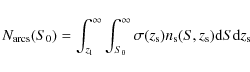
where
When sources are much smaller than the characteristic length over which the lensing properties of the deflector change significantly, they can be considered as pointlike. In this case the lens mapping can be linearized and the length-to-width ratio of the distorted images, d, is simply given by the ratio of the eigenvalues of the Jacobian matrix at image position. In this case the cross section for arcs with a higher length-to-width ratio than some threshold d0 is by definition the area of the lens plane where the eigenvalue ratio is greater than d0, mapped back to the source plane. This framework can be also easily modified to account for the extended size of real sources, by convolving the lensing properties over the typical source domain, assumed here to be circular with angular radius of 0.5''. Several studies have shown that the properties of the sources are relevant for determining the shape of gravitational arcs (see e.g. Gao et al. 2009; Meneghetti et al. 2008). Our method cannot take all the effects of source morphologies and luminosity profiles into account, however the intrinsic ellipticity of real sources is accounted for by the elegant algorithm proposed by Keeton (2001).
Because of the huge number of cross sections computed in this work, we
only focused on a single value for the length-to-width threshold, d0 = 7.5. While a distribution of thresholds would be preferable, we expect the change in d0
to produce only a shift in the normalization of cross sections, by
leaving every qualitative conclusion unchanged. As mentioned above, we
consider only one source redshift,
![]() .
.
We computed the strong lensing cross sections for each of the
49 366 high-resolution deflection angle maps, produced as
described in Sect. 3.1.
Many of them are vanishing, because, even though the deflector is able
to produce critical curves, they are small compared to the typical
source size to efficiently distort images. It turns out that only
6375 clusters have at least one projection with nonvanishing cross
section for
![]() .
In total, the cluster projections capable of large distortions are
11,347. The lensing cross sections range from a minimal value of
.
In total, the cluster projections capable of large distortions are
11,347. The lensing cross sections range from a minimal value of
![]() Mpc2 to a maximal value of
Mpc2 to a maximal value of
![]() Mpc2 (the properties of this super-lens shown in Appendix A). However, the vast majority of the lenses capable of producing giant arcs have cross sections larger than
Mpc2 (the properties of this super-lens shown in Appendix A). However, the vast majority of the lenses capable of producing giant arcs have cross sections larger than ![]()
![]() Mpc2, as seen in Fig. 1, where we show the distribution of the lensing cross sections for giant arcs among the clusters analyzed here.
Mpc2, as seen in Fig. 1, where we show the distribution of the lensing cross sections for giant arcs among the clusters analyzed here.
![\begin{figure}
\par\includegraphics[width=9cm]{Figures/14098fg1.eps}
\vspace*{2.5mm}
\end{figure}](/articles/aa/full_html/2010/11/aa14098-10/img74.png)
|
Figure 1:
The distribution of the lensing cross sections for giant arcs of all the strong lensing clusters between
|
| Open with DEXTER | |
Given the large number of clusters analyzed here and the computational
time required to analyze them, it was impossible to calculate the
lensing cross sections for several source redshifts. Thus it is not
easy to convert the lensing cross section into a number of arcs using
Eq. (8).
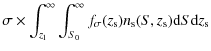
Nevertheless, we can estimate this number using some approximation. If
we assume that the lensing cross section evolves with redshift as
![]() ,
where
,
where ![]() is the lensing cross section for sources at
is the lensing cross section for sources at
![]() and
and
![]() is a scaling function, then the number of arcs detectable behind a cluster can be expressed as
is a scaling function, then the number of arcs detectable behind a cluster can be expressed as
In the last equation, we have introduced the effective source number density. Apart from the dependency on the scaling of the lensing cross section with the source redshift, which is discussed below, the effective source number density is set by the minimal surface brightness (i.e. flux per square arcsec) of detectable arcs. Thus, it is determined by the characteristics of the observation, i.e., by the throughput of the instrument and by the level of the background. Using the optical simulator SkyLens (Meneghetti et al. 2008,2010), we simulated a deep exposure of 8000 s with the Advanced Camera for Surveys onboard the Hubble Space Telescope in the F775W filter. This code uses the morphologies, the luminosities, and the redshifts of the galaxies in the Hubble Ultra-Deep-Field (Beckwith et al. 2006) to produce extremely realistic images of the sky including several observational noises. Setting the background level to 22.4 mag arcsec-2, the 1
![\begin{figure}
\par\mbox{\includegraphics[width=8.8cm]{Figures/14098fg2a.eps} \includegraphics[width=8.8cm]{Figures/14098fg2b.eps} }\vspace*{2.5mm}\end{figure}](/articles/aa/full_html/2010/11/aa14098-10/img83.png)
|
Figure 2:
Left panel: galaxy number counts per square arcmin in redshift
bins as obtained by simulating a deep observation of 8000 s with
HST/ACS in the F775W filter. The two histograms refer to two different SExtractor detection thresholds, namely S0=25.78 and S0=24.58 mag arcsec-2, which correspond to 1 |
| Open with DEXTER | |
The scaling function ![]() is expected to depend on several properties of the lenses, like their
redshifts, density profiles, ellipticity, and substructures. Therefore,
adopting a universal scaling law is certainly a gross approximation. On
the other hand, it is also useful to have a rough estimate of the
effective number density of sources to link a quantity like the cross
section, which is not directly measurable, to something that can be
observed, like the number of arcs behind a cluster. To estimate the
scaling function
is expected to depend on several properties of the lenses, like their
redshifts, density profiles, ellipticity, and substructures. Therefore,
adopting a universal scaling law is certainly a gross approximation. On
the other hand, it is also useful to have a rough estimate of the
effective number density of sources to link a quantity like the cross
section, which is not directly measurable, to something that can be
observed, like the number of arcs behind a cluster. To estimate the
scaling function ![]() for a cluster at reshift
for a cluster at reshift ![]() ,
we use a toy lens model with an NFW density profile and fixed projected ellipticity
,
we use a toy lens model with an NFW density profile and fixed projected ellipticity
![]() .
This ellipticity is introduced in the lensing potential as discussed in Meneghetti et al. (2003b).
Using the same algorithm used to analyze the deflection angle maps of
numerically simulated clusters, we measure how the lensing cross
section grows as a function of the source redshift. In the right panel
of Fig. 2, we show the scaling functions for a cluster with mass
.
This ellipticity is introduced in the lensing potential as discussed in Meneghetti et al. (2003b).
Using the same algorithm used to analyze the deflection angle maps of
numerically simulated clusters, we measure how the lensing cross
section grows as a function of the source redshift. In the right panel
of Fig. 2, we show the scaling functions for a cluster with mass
![]() at several redshifts between z = 0.2 and z = 0.8.
at several redshifts between z = 0.2 and z = 0.8.
The effective number counts derived as explained above are reported in Table 1 for different cluster masses and redshifts. As said above, the counts refer to an observation with HST/ACS in the F775W filter with an exposure time of 8000 s. In each column, the biggest and the smallest number correspond to detections at 1![]() and at 3
and at 3![]() above the background rms. First, the dependence on the mass is weak,
which allows extending the validity of these calculations to a broad
range of masses. Second, the rise of the scaling function for
increasing lens redshift compensates for the lower number of galaxies
at high redshift. Thus the effective source number counts do not drop,
but tend to increase as the lens redshift increases. Using Eq. (9), we can finally link the number of arcs expected for a given lensing cross section
above the background rms. First, the dependence on the mass is weak,
which allows extending the validity of these calculations to a broad
range of masses. Second, the rise of the scaling function for
increasing lens redshift compensates for the lower number of galaxies
at high redshift. Thus the effective source number counts do not drop,
but tend to increase as the lens redshift increases. Using Eq. (9), we can finally link the number of arcs expected for a given lensing cross section ![]() to the effective number density of background sources, i.e., to the
depth of the observation. For example, for a cluster with cross section
to the effective number density of background sources, i.e., to the
depth of the observation. For example, for a cluster with cross section
![]() Mpc2, the expected number of giant arcs varies from 0.3 to 1.6 for
Mpc2, the expected number of giant arcs varies from 0.3 to 1.6 for
![]() in the range
[40-200]. Conversely, in Fig. 3 we show the lensing cross section required for
in the range
[40-200]. Conversely, in Fig. 3 we show the lensing cross section required for
![]() as a function of the effective number density of background sources.
Even for very high effective number counts (or equivalently very deep
exposures), the lensing cross section needs to be very large in order
to expect at least one arc behind a galaxy cluster. For example, for a
cross section of
as a function of the effective number density of background sources.
Even for very high effective number counts (or equivalently very deep
exposures), the lensing cross section needs to be very large in order
to expect at least one arc behind a galaxy cluster. For example, for a
cross section of
![]() Mpc2, the effective number density of background sources needs to be
Mpc2, the effective number density of background sources needs to be ![]() 130 galaxies per square arcmin. This number density needs to be doubled to expect to observe two arcs, and so forth.
130 galaxies per square arcmin. This number density needs to be doubled to expect to observe two arcs, and so forth.
In the rest of the paper, we use the lensing cross section to distinguish between lenses of different strengths. Observationally, the lensing cross section is not a directly measurable quantity. A possible method of estimating the lensing cross section is through the detailed parametric reconstruction of the lens potential (Meneghetti et al., in prep.). Indeed, the deflection field can be readily derived from the lensing potential and used to measure the lensing cross section using the same method as was adopted in our simulations. Other methods of defining the strength of the lenses may be based on quantities that are more directly measurable, like the angular separations of multiple images, which can be used to estimate the size of the critical lines, etc. However, in this paper, given the huge size of the cluster sample considered, we could not explore this other possibility.
Table 1: Effective galaxy number counts per square arcmin behind clusters with different masses and redshifts.
4 Cluster masses
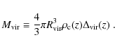
The easiest way to characterize a cluster lens is through its mass. In
the following, we refer to the cluster mass as the mass contained in
spheres of radius
![]() .
This virial radius encloses a density of
.
This virial radius encloses a density of
![]() times the closure density of the Universe at the redshift of the cluster,
times the closure density of the Universe at the redshift of the cluster,
![\begin{displaymath}\rho_{\rm c} (z)=\frac{3 H_0^2}{8 \pi G}\left[ \Omega_{\rm m}(1+z)^3+\Omega_\Lambda \right] ,
\end{displaymath}](/articles/aa/full_html/2010/11/aa14098-10/img99.png)
|
(10) |
where H0 is the present value of the Hubble constant, z the redshift, and G the gravitational constant. The virial overdensity
|
(11) |
As an alternative to the virial mass, different mass definitions are often adopted in literature, such as the mass corresponding to a constant overdensity
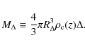
|
(12) |
The mass function of objects in the M AREN OSTRUM U NIVERSE is in very good agreement with the theoretical expectations (Gottlöber et al. 2008; Sheth & Tormen 2002). This is shown in Fig. 4, where the number of halos above a minimal virial mass is shown for different redshifts and compared to the predictions of the Sheth & Tormen mass function at redshift z=0. At this redshift more than 4000 cluster-sized objects with masses higher than
Selecting the clusters via their strong lensing efficiency implies that
only the high mass tail of the distribution is properly sampled.
Indeed, since the amplitude of the gravitational deflection depends
directly on the mass, strong lenses are the most massive objects at
each epoch. In particular, we expect a minimal mass below which
clusters do not develop critical lines and are unable to produce very
distorted images like gravitational arcs. Since clusters must be
located at a convenient angular diameter distance between the observer
and the sources, the number and the typical mass of strong lensing
clusters should vary as a function of both the lens and the source
redshifts. Assuming a fixed source redshift of
![]() ,
the mass distribution of strong lensing clusters in a comoving volume of
,
the mass distribution of strong lensing clusters in a comoving volume of
![]() Mpc3 at different redshifts is given in the left panel of Fig. 5. The color levels show the number counts of critical clusters in the
Mpc3 at different redshifts is given in the left panel of Fig. 5. The color levels show the number counts of critical clusters in the
![]() plane. Lighter (darker) colors correspond to smaller (larger) number
counts. The outer dotted contour show the limits of the distribution:
no critical clusters have been found outside the region enclosed by
this line. The two inner contours correspond to the 50% and to
the 90% of the peak of the distribution. Thus, they show how
rapidly the critical cluster counts decrease as a function of both mass
and redshift. As the figure shows, the region of the plane where
clusters are able to produce critical lines extends down to masses of
groups at the most favorable redshifts. However, these are very rare
objects. At redshifts higher than 1.2, or lower that 0.2, the mass
threshold grows rapidly, while the number counts of critical clusters
drop. These lenses are too close to the sources or to the observer to
be critical.
plane. Lighter (darker) colors correspond to smaller (larger) number
counts. The outer dotted contour show the limits of the distribution:
no critical clusters have been found outside the region enclosed by
this line. The two inner contours correspond to the 50% and to
the 90% of the peak of the distribution. Thus, they show how
rapidly the critical cluster counts decrease as a function of both mass
and redshift. As the figure shows, the region of the plane where
clusters are able to produce critical lines extends down to masses of
groups at the most favorable redshifts. However, these are very rare
objects. At redshifts higher than 1.2, or lower that 0.2, the mass
threshold grows rapidly, while the number counts of critical clusters
drop. These lenses are too close to the sources or to the observer to
be critical.
Requiring that clusters are also able to produce giant arcs produces an
additional selection effect. Using the same convention as for the
dotted contours, the solid contours refer to arcs with nonvanishing
cross-sections for giant arcs. There are no clusters at
![]() that are able to produce large distortions, although they could be
still efficient for sources at much higher redshift. The most massive
clusters in the box are still able to develop small critical lines up
to
that are able to produce large distortions, although they could be
still efficient for sources at much higher redshift. The most massive
clusters in the box are still able to develop small critical lines up
to
![]() .
The bulk of clusters producing giant arcs is concentrated at
.
The bulk of clusters producing giant arcs is concentrated at
![]() .
Finally, the dashed contours show the distribution of the lenses with lensing cross sections above
.
Finally, the dashed contours show the distribution of the lenses with lensing cross sections above
![]() Mpc2.
These lenses are likely to be the most easily targeted for strong
lensing studies and contribute significantly to the lensing signal in
the universe given that, as discussed in the previous section, the
expected number of strong lensing features produced by these objects is
by far greater than for lenses with smaller cross sections. These, on
the other hand, are more abundant, so they will dominate the total
lensing optical depth. As shown by the contours, these objects are
confined in a smaller area on the
Mpc2.
These lenses are likely to be the most easily targeted for strong
lensing studies and contribute significantly to the lensing signal in
the universe given that, as discussed in the previous section, the
expected number of strong lensing features produced by these objects is
by far greater than for lenses with smaller cross sections. These, on
the other hand, are more abundant, so they will dominate the total
lensing optical depth. As shown by the contours, these objects are
confined in a smaller area on the
![]() plane. They are typically clusters with masses exceeding a few times
plane. They are typically clusters with masses exceeding a few times
![]() and with redshift below unity. Most of them are concentrated in a narrow redshift window between 0.2<z<0.6.
and with redshift below unity. Most of them are concentrated in a narrow redshift window between 0.2<z<0.6.
![\begin{figure}
\par\includegraphics[width=9cm]{Figures/14098fg3.eps}
\vspace*{2.5mm}\end{figure}](/articles/aa/full_html/2010/11/aa14098-10/img113.png)
|
Figure 3: The lensing cross section required for an expectation value of one giant arc behind a cluster as a function of the effective number of background sources. |
| Open with DEXTER | |
![\begin{figure}
\par\includegraphics[width=7.4cm,clip]{Figures/14098fg4.eps}
\vspace*{2.5mm}\end{figure}](/articles/aa/full_html/2010/11/aa14098-10/img114.png)
|
Figure 4: The number of halos above a given mass within the M AREN OSTRUM U NIVERSE simulation box at four different redshifts between 0 and 2. The dotted line shows the theoretical expectations from the Sheth & Tormen mass function. |
| Open with DEXTER | |
Although we see an interesting selection effect in the 3D masses,
what really matters for strong lensing is the projected mass, in
particular, the mass contained in a cylinder around the cluster center,
where the critical lines form. For each cluster in our sample, we
measure the projected mass within R2500,
![]() ,
for each of the three projections used for ray-tracing. This is defined as that of a sphere encompassing a mean density of
,
for each of the three projections used for ray-tracing. This is defined as that of a sphere encompassing a mean density of
![]() .
Typically, it corresponds to a region that is large enough to contain
the cluster critical lines. Here, the projected mass is obtained by
integrating all the mass in a cylinder of height
.
Typically, it corresponds to a region that is large enough to contain
the cluster critical lines. Here, the projected mass is obtained by
integrating all the mass in a cylinder of height ![]() Mpc. We show the distribution of the strong lensing clusters in the plane
Mpc. We show the distribution of the strong lensing clusters in the plane
![]() in the right panel of Fig. 5.
Interestingly, although it appears clear that strong lensing depends on
the mass in the central region of the deflectors, the spread in
projected mass is wider by about one order-of-magnitude than in 3D.
There are clusters that have relatively low mass projected into the
core but that are still capable of producing strong lensing effects of
different intensities. We interpret this result as being due to the
importance that other properties of the lenses have for strong lensing,
like the amount of substructures and the level of asymmetry and
ellipticity in the cluster cores, as shown in Meneghetti et al. (2007a).
In several cases, and especially for clusters producing mild strong
lensing effects (i.e. clusters with critical curves), the excess of
shear produced by a clumpy and asymmetric mass distribution can
compensate for the low value of the central convergence.
in the right panel of Fig. 5.
Interestingly, although it appears clear that strong lensing depends on
the mass in the central region of the deflectors, the spread in
projected mass is wider by about one order-of-magnitude than in 3D.
There are clusters that have relatively low mass projected into the
core but that are still capable of producing strong lensing effects of
different intensities. We interpret this result as being due to the
importance that other properties of the lenses have for strong lensing,
like the amount of substructures and the level of asymmetry and
ellipticity in the cluster cores, as shown in Meneghetti et al. (2007a).
In several cases, and especially for clusters producing mild strong
lensing effects (i.e. clusters with critical curves), the excess of
shear produced by a clumpy and asymmetric mass distribution can
compensate for the low value of the central convergence.
5 Halo triaxiality and orientation
Since simulated galaxy clusters are triaxial (see e.g. Gottlöber & Yepes 2007; Jing & Suto 2000),
their projected mass depends on their orientation with respect to the
line of sight. In order to evaluate how this affects the strong lensing
ability of clusters, we measured their triaxial best fit model and
discuss the correlation of the orientation with the occurrence of
critical lines and giant arcs. To do that, we measured the moment of
inertia tensor Iij of each cluster in the sample. The cluster particles within
![]() were sorted in a regular cubic grid of
were sorted in a regular cubic grid of
![]() cells. The mass density in each grid cell was then computed The inertial tensor components are given by
cells. The mass density in each grid cell was then computed The inertial tensor components are given by
|
(13) |
where mk is the mass of in the kth selected cell and R=[Ri] is the vector that identifies the cell position with respect to the center of mass of the system. The triaxial model of the cluster and its principal axes were obtained by diagonalizing the inertial tensor, finding its eigenvalues and eigenvectors.
![\begin{figure}
\par\mbox{\includegraphics[width=8.8cm]{Figures/14098fg5a.eps}\includegraphics[width=8.8cm]{Figures/14098fg5b.eps} }\vspace*{2.5mm}\end{figure}](/articles/aa/full_html/2010/11/aa14098-10/img120.png)
|
Figure 5:
The distributions of strong lensing clusters in the
|
| Open with DEXTER | |
The fits show that clusters have prolate triaxial halos, and the
distributions of the axis ratios of strong lensing clusters are not
significantly different from that expected for the general cluster
population (see e.g. Jing & Suto 2002). This agrees with the results of Hennawi et al. (2007),
who also find that strong lensing clusters are not significantly more
triaxial than normal clusters. However, strong lensing clusters seem to
be affected by an orientation bias. In Fig. 6,
we show the cumulative probability distribution function of the angle
between the major axes of the inertial ellipsoid and the line of sight
to the cluster for the whole sample of lensing clusters and for the
subsample of clusters producing giant arcs.
We also show the distribution of the orientation angles of the most
efficient lenses in the sample, i.e. with lensing cross section
![]() Mpc2.
We also display, the distribution corresponding to totally randomly
oriented lenses. We find that lensing clusters tend to be aligned with
the line of sight. This orientation bias increases with the strength of
the lens: the median angle for critical clusters is
Mpc2.
We also display, the distribution corresponding to totally randomly
oriented lenses. We find that lensing clusters tend to be aligned with
the line of sight. This orientation bias increases with the strength of
the lens: the median angle for critical clusters is ![]()
![]() ,
while, for the subsample of clusters capable of producing giant arcs, the median angle is
,
while, for the subsample of clusters capable of producing giant arcs, the median angle is ![]()
![]() .
The median decreases to
.
The median decreases to ![]()
![]() for clusters with lensing cross section
for clusters with lensing cross section
![]() Mpc2. In the case of random orientation we should expect a median angle of
Mpc2. In the case of random orientation we should expect a median angle of ![]() .
This is an important effect, which can affect the conclusions of many
studies aiming at estimating the mass of clusters through strong
lensing or at measuring cosmological parameters using the abundance of
highly elongated arcs on the sky. In fact, we expect that, owing to the
orientation bias, 3D strong-lensing masses are biased high, if the
approximation of spherical symmetry is used to convert the measured 2D
into 3D mass profiles. Moreover, this alignment bias has to be
properly modeled when estimating the lensing optical depth for a
population of strong lenses in a given cosmology. Similar results have
been found by Hennawi et al. (2007).
They also find a correlation between strong lensing and orientation of
the lenses and similar distributions of the orientation angles to those
we find here.
.
This is an important effect, which can affect the conclusions of many
studies aiming at estimating the mass of clusters through strong
lensing or at measuring cosmological parameters using the abundance of
highly elongated arcs on the sky. In fact, we expect that, owing to the
orientation bias, 3D strong-lensing masses are biased high, if the
approximation of spherical symmetry is used to convert the measured 2D
into 3D mass profiles. Moreover, this alignment bias has to be
properly modeled when estimating the lensing optical depth for a
population of strong lenses in a given cosmology. Similar results have
been found by Hennawi et al. (2007).
They also find a correlation between strong lensing and orientation of
the lenses and similar distributions of the orientation angles to those
we find here.
Apart from the orientation, the halo triaxiality is important because
it determines the projected shape of the lenses.
It has been shown in several papers that, for a fixed mass, the strong
lensing cross section is larger for higher ellipticities of the
projected mass distribution (Meneghetti et al. 2007a,2003b).
With such a large sample of lensing clusters, we can address the
question the distribution of their projected ellipticities. These are
measured as for the 3D shape of the lenses. We measured and
diagonalized the inertial tensor of the cluster mass distribution
projected on a regular grid of
![]() cells.
We selected those cells where the surface density exceeds some
thresholds. The thresholds we used are given by the mean surface
densities at
cells.
We selected those cells where the surface density exceeds some
thresholds. The thresholds we used are given by the mean surface
densities at
![]() and at
and at
![]() .
Thus, we measured the projected ellipticity both in the outer and in the inner cluster regions.
.
Thus, we measured the projected ellipticity both in the outer and in the inner cluster regions.
The probability distribution functions of the projected ellipticity are shown in Fig. 7. The ellipticity is defined as
![]() ,
where a and b are the major and minor axes of the ellipse. The lines refer to critical clusters (assuming again a source redshift of
,
where a and b are the major and minor axes of the ellipse. The lines refer to critical clusters (assuming again a source redshift of
![]() ), to clusters with nonvanishing cross section for giant arcs, and to clusters with large cross section for giant arcs (>
), to clusters with nonvanishing cross section for giant arcs, and to clusters with large cross section for giant arcs (>
![]() Mpc2).
The left and the right panels show the distributions of the outer and
of the inner ellipticities. We find that the projected cores are more
elliptical, with distributions that peak at
Mpc2).
The left and the right panels show the distributions of the outer and
of the inner ellipticities. We find that the projected cores are more
elliptical, with distributions that peak at
![]() .
It is interesting to note that critical clusters have a bimodal
ellipticity distribution: several clusters have extremely elongated
cores with ellipticities that extend to
.
It is interesting to note that critical clusters have a bimodal
ellipticity distribution: several clusters have extremely elongated
cores with ellipticities that extend to
![]() .
Since we are fitting each lens with a single ellipse, these are mainly
clusters with substructures near the centers that mimic high
ellipticities. We recall that the tangential critical lines form where
.
Since we are fitting each lens with a single ellipse, these are mainly
clusters with substructures near the centers that mimic high
ellipticities. We recall that the tangential critical lines form where
| (14) |
As discussed in Torri et al. (2004), the shear produced by the substructures enhance the ability of the clusters to produce strong lensing, because it makes critical even those lenses where the convergence is not enough to ensure it (
At large radii, we find that the ellipticities are lower and the projected ellipticity becomes lower as the strength of the lens increases. This is clearly related to the orientation bias discussed above. The strongest lenses are typically elongated along the line of sight, making them appear rounder on the sky.
![\begin{figure}
\par\includegraphics[width=7cm,clip]{Figures/14098fg6.eps}
\end{figure}](/articles/aa/full_html/2010/11/aa14098-10/img131.png)
|
Figure 6:
The cumulative probability distribution function of the angles between the major axes of the strong lenses in the M AREN OSTRUM U NIVERSE
and the line of sight. Shown are the results for the clusters with
critical lines, (solid line), for the clusters with cross section for
giant arcs larger than zero (dot-dashed line), and for the clusters
with cross section for giant arcs larger than
|
| Open with DEXTER | |
![\begin{figure}
\par\mbox{\includegraphics[width=8.8cm]{Figures/14098fg7a.eps} \includegraphics[width=8.8cm]{Figures/14098fg7b.eps} }\vspace*{3mm}\end{figure}](/articles/aa/full_html/2010/11/aa14098-10/img132.png)
|
Figure 7:
The probability density functions of the projected ellipticity of the lensing clusters in the M AREN OSTRUM U NIVERSE.
Shown are the results for the clusters with critical lines (solid
lines), for the subsample of clusters with nonvanishing cross sections
for giant arcs (dot-dashed lines), and for cluster with
|
| Open with DEXTER | |
![\begin{figure}
\par\mbox{\includegraphics[width=8.8cm]{Figures/14098fg8a.eps}\includegraphics[width=8.8cm]{Figures/14098fg8b.eps} }\end{figure}](/articles/aa/full_html/2010/11/aa14098-10/img133.png)
|
Figure 8: NFW concentrations as a function of the halo mass and redshift. Left and right panels refer to clusters with critical lines and to clusters with nonvanishing lensing cross section for giant arcs, respectively. The concentrations are normalized to those measured on the whole sample of clusters in the simulation box, regardless of their ability to produce strong lensing effects. Different colors are used to encode the different values of the normalized concentrations. The labeled contours provide the link between the color scale and the concentration values. |
| Open with DEXTER | |
![\begin{figure}
\par\mbox{\includegraphics[width=8.8cm]{Figures/14098fg9a.eps}\in...
...cludegraphics[width=8.8cm]{Figures/14098fg9d.eps} }\vspace*{2.5mm}\end{figure}](/articles/aa/full_html/2010/11/aa14098-10/img135.png)
|
Figure 9:
Same as in Fig. 8,
but showing 2D-concentrations of lensing clusters. The
2D-concentrations have been normalized to the 3D-concentrations of the
whole cluster sample. Starting from the top-left panel, we
show the 2D-concentrations as a function of mass and redshift
for 1) clusters with critical lines; 2) clusters with
nonvanishing lensing cross sections for giant arcs; 3) clusters
with cross section
|
| Open with DEXTER | |
6 Concentrations
Several previous studies have discussed the importance of the halo concentration for lensing. Using simulations, Hennawi et al. (2007) find that concentrations of lensing clusters are on average ![]()
![]() higher than the typical clusters in the universe. Broadhurst et al. (2008) report a very high level of mass concentrations (
higher than the typical clusters in the universe. Broadhurst et al. (2008) report a very high level of mass concentrations (![]() )
in a sample of four well-known strong lensing clusters. Fedeli et al. (2007b) show that, at a given mass, the strong lenses are
)
in a sample of four well-known strong lensing clusters. Fedeli et al. (2007b) show that, at a given mass, the strong lenses are ![]()
![]() to
to ![]()
![]() more concentrated than the average. Here, we discuss the concentrations of the clusters in the M AREN OSTRUM U NIVERSE.
more concentrated than the average. Here, we discuss the concentrations of the clusters in the M AREN OSTRUM U NIVERSE.
We measured the concentrations by fitting the density profiles of the clusters in our sample with the Navarro-Frenk-White (Navarro et al. 1997) formula,
|
(15) |
where
Instead of fitting the density profiles of individual halos, which are
noisy, we prefer to fit the stacked profiles of clusters with similar
redshifts and masses. The mass bins are equally spaced on a logarithmic
scale. We stack the profiles of all clusters in the mass bins and
perform the NFW fit. Again, we select those objects that exhibit
critical lines for sources at
![]() ,
and, among them, those halos that are also able to produce large
distortions, with lensing cross section above some minimal value. The
concentrations of the clusters in these two subsamples are compared
with those of general clusters, regardless of their ability to behave
as strong lenses. The results are shown in Fig. 8.
The left and the right panels refer to critical and to large distortion
clusters, respectively. The color intensity reflects the amplitude of
the concentrations. The concentrations are normalized to those of
general clusters of similar mass and redshifts. The labels in the
overlaid contours indicate the numerical value of the normalized
concentration at the corresponding color level. Strong lensing clusters
at moderate redshifts have concentrations similar to those of the
general cluster population. Only low-mass lenses have a relatively low
concentration bias (
,
and, among them, those halos that are also able to produce large
distortions, with lensing cross section above some minimal value. The
concentrations of the clusters in these two subsamples are compared
with those of general clusters, regardless of their ability to behave
as strong lenses. The results are shown in Fig. 8.
The left and the right panels refer to critical and to large distortion
clusters, respectively. The color intensity reflects the amplitude of
the concentrations. The concentrations are normalized to those of
general clusters of similar mass and redshifts. The labels in the
overlaid contours indicate the numerical value of the normalized
concentration at the corresponding color level. Strong lensing clusters
at moderate redshifts have concentrations similar to those of the
general cluster population. Only low-mass lenses have a relatively low
concentration bias (![]()
![]() ).
The bias become more significant at low and high redshifts, where it
also affects the largest masses. Because of their short distance to the
observer or to the sources, these clusters need to be very concentrated
to focus the light from distant sources. The bias is mass dependent. As
the mass decreases, the bias is stronger. This isa clear selection
effect: if we require a cluster to be critical or even to produce large
arcs, only the most concentrated halos in the lowest mass bins are able
to satisfy the requirement.
).
The bias become more significant at low and high redshifts, where it
also affects the largest masses. Because of their short distance to the
observer or to the sources, these clusters need to be very concentrated
to focus the light from distant sources. The bias is mass dependent. As
the mass decreases, the bias is stronger. This isa clear selection
effect: if we require a cluster to be critical or even to produce large
arcs, only the most concentrated halos in the lowest mass bins are able
to satisfy the requirement.
As mentioned above, lensing probes the projected mass distribution of
clusters. The concentrations are typically measured by fitting multiple
image systems and arcs with combinations of projected parametric
models. Then, the 3D density profiles are determined by assuming
spherical symmetry. As we discussed earlier, clusters have triaxial
shapes, thus the assumption of spherical symmetry is generally wrong.
Moreover, as we have shown in the previous section, strong lensing
clusters tend to be seen along their major axes. For these reasons, the
concentrations measured in 2D through strong lensing are expected to be
more biased than 3D concentrations. This effect is also discussed in Hennawi et al. (2007),
where a comparison of 2D vs. 3D concentrations of individual
clusters led to the conclusion that the former are typically ![]()
![]() higher than the latter. To verify this result, we proceed to fit the
surface density profiles of our strong lensing clusters in their
projections. Again, to do this, we stack the profiles in mass and
redshift bins. The fitting formula is given by the truncated NFW
surface density profile (Meneghetti et al. 2000),
higher than the latter. To verify this result, we proceed to fit the
surface density profiles of our strong lensing clusters in their
projections. Again, to do this, we stack the profiles in mass and
redshift bins. The fitting formula is given by the truncated NFW
surface density profile (Meneghetti et al. 2000),
where

|
(17) |
where
![$\displaystyle -\frac{2}{(x^2-1)^{3/2}}
\arctan\left[\frac{x-1}{\sqrt{x^2-1}}
\tanh\left(\frac{u}{2}\right)\right]$](/articles/aa/full_html/2010/11/aa14098-10/img154.png)
if x>1;
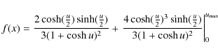
if x=1; and
![$\displaystyle \frac{2}{{(1-x^2)}^{3/2}}
\mbox{arctanh}\left[\frac{1-x}{\sqrt{1-x^2}}
\tanh\left(\frac{u}{2}\right)\right]$](/articles/aa/full_html/2010/11/aa14098-10/img157.png)
if x<1. In the previous formulae,
The resulting 2D concentrations, for several classes of strong lenses,
as a function of mass and redshift are shown in Fig. 9. As done in Fig. 8,
the 2D-concentrations are normalized to the 3D concentrations of
general clusters of similar masses and redshifts. Starting from the
top-left panel, we show the results for clusters with critical lines
and for clusters with lensing cross sections for giant arcs larger than
0,
![]() Mpc2, and
Mpc2, and
![]() Mpc2,
respectively. As expected, the bias grows compared to the 3D case, and
the amount by which it increases depends on the class of lensing
clusters we are considering. For critical clusters, the ratios between
2D concentrations and the corresponding 3D concentrations are
Mpc2,
respectively. As expected, the bias grows compared to the 3D case, and
the amount by which it increases depends on the class of lensing
clusters we are considering. For critical clusters, the ratios between
2D concentrations and the corresponding 3D concentrations are ![]() 1.2
for intermediate redshift clusters, but they become higher
than 1.3 at low and at high redshifts. For clusters able to
produce giant arcs, the 2D-concentration bias is significantly higher.
As discussed for the 3D concentrations, the amplitude of the bias
depends on both redshift and mass: lower masses at short distances from
the observer or from the sources have the largest biases. Moreover,
increasing the lensing cross section for giant arcs, the concentration
bias grows dramatically. For example, massive clusters (
1.2
for intermediate redshift clusters, but they become higher
than 1.3 at low and at high redshifts. For clusters able to
produce giant arcs, the 2D-concentration bias is significantly higher.
As discussed for the 3D concentrations, the amplitude of the bias
depends on both redshift and mass: lower masses at short distances from
the observer or from the sources have the largest biases. Moreover,
increasing the lensing cross section for giant arcs, the concentration
bias grows dramatically. For example, massive clusters (
![]() )
at the most efficient redshifts for strongly lensing sources at
)
at the most efficient redshifts for strongly lensing sources at
![]() (
(
![]() )
with lensing cross sections larger than
)
with lensing cross sections larger than
![]() Mpc2 have 2D-concentrations that are typically higher by
Mpc2 have 2D-concentrations that are typically higher by ![]()
![]() than
the 3D-concentration of general clusters. For lower masses and
redshifts, the 2D-concentrations can be higher than expected in 3D by
more than a factor of two. This is a consequence of the orientation
bias discussed in the previous section. To be able to produce large and
very elongated arcs, clusters lying too close to the observer or to the
source must be optimally oriented and extremely concentrated. Due to
triaxiality, the concentrations measured from the 2D mass distributions
of these clusters are much higher than the correspondent 3D
concentrations (Oguri et al. 2005; Gavazzi 2005).
As discussed in Sect. 3.3, a lensing cross section of
than
the 3D-concentration of general clusters. For lower masses and
redshifts, the 2D-concentrations can be higher than expected in 3D by
more than a factor of two. This is a consequence of the orientation
bias discussed in the previous section. To be able to produce large and
very elongated arcs, clusters lying too close to the observer or to the
source must be optimally oriented and extremely concentrated. Due to
triaxiality, the concentrations measured from the 2D mass distributions
of these clusters are much higher than the correspondent 3D
concentrations (Oguri et al. 2005; Gavazzi 2005).
As discussed in Sect. 3.3, a lensing cross section of
![]() Mpc2 corresponds to an expectation value of
Mpc2 corresponds to an expectation value of ![]() 1 giant arc in a deep HST observation. Clusters like A1689, which contains about 10 arcs with a length-to-width ratio greater than 7.5 (Sand et al. 2005),
are thus expected to have extremely large lensing cross sections. If
the properties of real clusters are reproduced correctly by the
clusters in our simulations, these very efficient strong lenses are
likely to have extremely biased 2D-concentrations, as recently reported
by Broadhurst et al. (2008) (see also Oguri et al. 2009). Our findings agree with the results recently published by Oguri & Blandford (2009),
who use semi-analytic models of triaxial halos to estimate that the
projected mass distributions of strong lensing clusters have
1 giant arc in a deep HST observation. Clusters like A1689, which contains about 10 arcs with a length-to-width ratio greater than 7.5 (Sand et al. 2005),
are thus expected to have extremely large lensing cross sections. If
the properties of real clusters are reproduced correctly by the
clusters in our simulations, these very efficient strong lenses are
likely to have extremely biased 2D-concentrations, as recently reported
by Broadhurst et al. (2008) (see also Oguri et al. 2009). Our findings agree with the results recently published by Oguri & Blandford (2009),
who use semi-analytic models of triaxial halos to estimate that the
projected mass distributions of strong lensing clusters have ![]()
![]() higher concentrations than typical clusters with similar redshifts and masses (see also Sereno et al. 2010).
higher concentrations than typical clusters with similar redshifts and masses (see also Sereno et al. 2010).
7 X-ray luminosities
Gas physics are known to be potentially very important for strong lensing (see e.g. Puchwein et al. 2005; Hilbert et al. 2008).
Several processes taking place in the intra-cluster-medium (ICM), such
cooling, heating, energy feedback from AGNs and supernovae, and thermal
conduction can also affect the distribution of the dark matter in
clusters, influencing the shape of the density profiles (Dolag et al. 2004; Puchwein & Hilbert 2009; Yepes et al. 2007),
as well as the triaxiality of the dark matter halos. Phenomena such
cooling, star formation, and energy feedback change the thermal
properties of the ICM, thus influencing the X-ray emissivity. In fact,
several numerical studies report that X-ray luminosities in
nonradiative simulations are higher than in simulations where cooling
and feedback are active, while the
![]() relation derived from the same simulations is shallower than observed (e.g. Short et al. 2010; Mantz et al. 2008).
The extreme complexity of the processes involved presents a serious
challenge for simulating them accurately in a cosmological setting
(e.g. Borgani et al. 2004). Nevertheless, a nonradiative simulation like the M AREN OSTRUM U NIVERSE
can also provide useful qualitative information on the possible
correlation between strong lensing and X-ray emission by galaxy
clusters. Here, we focus in particular on the X-ray luminosity, which
is often used to select clusters for strong lensing surveys (e.g. Luppino et al. 1999).
relation derived from the same simulations is shallower than observed (e.g. Short et al. 2010; Mantz et al. 2008).
The extreme complexity of the processes involved presents a serious
challenge for simulating them accurately in a cosmological setting
(e.g. Borgani et al. 2004). Nevertheless, a nonradiative simulation like the M AREN OSTRUM U NIVERSE
can also provide useful qualitative information on the possible
correlation between strong lensing and X-ray emission by galaxy
clusters. Here, we focus in particular on the X-ray luminosity, which
is often used to select clusters for strong lensing surveys (e.g. Luppino et al. 1999).
![\begin{figure}
\par\includegraphics[width=9cm]{Figures/14098fg10.eps}
\vspace*{2.5mm}\end{figure}](/articles/aa/full_html/2010/11/aa14098-10/img169.png)
|
Figure 10:
The distribution of clusters with critical lines (dotted contours and
color levels), with non-vanishing cross section for giant arcs, and
with large lensing cross sections for giant arcs (solid contours),
|
| Open with DEXTER | |
The X-ray bolometric luminosity is calculated from the temperature and
internal energy of each gas particle in the simulated clusters. In
short, the X-ray luminosity is the sum of the contributions to the
emissivity from each gas particle,
![]() ,
where the sum extends over all the particles within
,
where the sum extends over all the particles within
![]() .
The emissivity of each gas element can be written as
.
The emissivity of each gas element can be written as
| (21) |
where
![\begin{figure}
\par\includegraphics[width=18cm]{Figures/14098fg11.eps}
\vspace*{5mm}
\end{figure}](/articles/aa/full_html/2010/11/aa14098-10/img178.png)
|
Figure 11: The relation between the X-ray bolometric luminosity and the cluster mass. Results are shown in four different redshift bins, as indicated at the top of each panel. Black, red, and blue data points (and errorbars) refer to the subsamples of critical and large distortion lenses. |
| Open with DEXTER | |
The distribution of strong lensing clusters in the
![]() plane is shown in Fig. 10, where we use the same notation as in Fig. 5. Again the counts correspond to the comoving volume of the M AREN OSTRUM U NIVERSE. Not surprisingly, given that the X-ray luminosity scales with the cluster mass (e.g. Kaiser 1986), the distribution of the strong lenses in the
plane is shown in Fig. 10, where we use the same notation as in Fig. 5. Again the counts correspond to the comoving volume of the M AREN OSTRUM U NIVERSE. Not surprisingly, given that the X-ray luminosity scales with the cluster mass (e.g. Kaiser 1986), the distribution of the strong lenses in the
![]() plane is very similar to that in the M-z
plane. As found for the masses, at each redshift a minimal X-ray
luminosity exists below which no critical lenses are found. The
``critical'' X-ray luminosity reaches a minimum between
plane is very similar to that in the M-z
plane. As found for the masses, at each redshift a minimal X-ray
luminosity exists below which no critical lenses are found. The
``critical'' X-ray luminosity reaches a minimum between
![]() and
and
![]() .
When we increase the minimal lensing cross section, the distributions
of clusters producing giant arcs moves upwards and shrinks along the
redshift axis.
.
When we increase the minimal lensing cross section, the distributions
of clusters producing giant arcs moves upwards and shrinks along the
redshift axis.
We now explore the scaling of the X-ray luminosity with the mass for strong lensing clusters in more details. In Fig. 11 we show the
![]() relation for four redshift bins, namely
relation for four redshift bins, namely
![]() ,
,
![]() ,
,
![]() ,
and
,
and
![]() .
Numerical simulations are known to be poor at describing the X-ray properties of the cosmic structures on the scales of groups (Borgani et al. 2008). Thus, we limit our analysis to clusters of masses
.
Numerical simulations are known to be poor at describing the X-ray properties of the cosmic structures on the scales of groups (Borgani et al. 2008). Thus, we limit our analysis to clusters of masses
![]() .
The
.
The
![]() relations found for clusters with critical lines, with nonvanishing
cross sections for giant arcs, and with lensing cross sections
relations found for clusters with critical lines, with nonvanishing
cross sections for giant arcs, and with lensing cross sections
![]() Mpc2 are shown. We find that, increasing the strong lensing efficiency, the slope of the
Mpc2 are shown. We find that, increasing the strong lensing efficiency, the slope of the
![]() relation changes, becoming smaller especially at the lowest masses.
This effect is also redshift-dependent, because it is more extreme in
the lowest and in the highest redshift bins. It shows that at the least
favorable redshifts for strong lensing, the X-ray luminosities of the
strong lensing clusters tend to be higher than for the general cluster
population, especially if the lens mass is relatively low. This seems
to suggest that some cluster property rather than the mass plays an
important role for boosting the lensing cross sections of these small
lenses, which also influences their X-ray luminosity. As discussed in Torri et al. (2004) and in Fedeli & Bartelmann (2007), mergers are likely to explain the effect we observe here.
relation changes, becoming smaller especially at the lowest masses.
This effect is also redshift-dependent, because it is more extreme in
the lowest and in the highest redshift bins. It shows that at the least
favorable redshifts for strong lensing, the X-ray luminosities of the
strong lensing clusters tend to be higher than for the general cluster
population, especially if the lens mass is relatively low. This seems
to suggest that some cluster property rather than the mass plays an
important role for boosting the lensing cross sections of these small
lenses, which also influences their X-ray luminosity. As discussed in Torri et al. (2004) and in Fedeli & Bartelmann (2007), mergers are likely to explain the effect we observe here.
8 Cluster's dynamical state
In this section, we use indicators of the virial and of the hydrostatic equilibria in clusters to investigate wether there is a correlation between strong lensing and dynamical activity in the lenses.
8.1 Virial equilibrium
The virial equilibrium is perhaps the most natural choice when trying to quantify the dynamical state of a bound structure. In the case of self-gravitating systems, this is quantified by the competition between the total potential energy and (twice) the internal kinetic energy.
In agreement with the scalar virial theorem and following Shaw et al. (2006), we introduce the parameter ![]() for the simulated clusters, defined as
for the simulated clusters, defined as
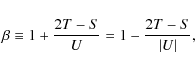
|
(22) |
where T is the internal kinetic energy, U the potential energy, and S a surface pressure term that arises from considering the structure as contained in a limited region (in this case the finite sphere). If

and the potential energy is given by
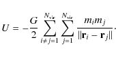
In Eqs. (23) and (24) mi,
The surface term, S, is computed by selecting the outermost 20% of the particles that are inside
![]() .
Let us call Q0.8 this set of particles. If R0.8 and R0.9 are the innermost and the median distances from the cluster center of the particles within Q0.8, respectively, then
.
Let us call Q0.8 this set of particles. If R0.8 and R0.9 are the innermost and the median distances from the cluster center of the particles within Q0.8, respectively, then
|
(25) |
where the sum is now extended to all the particles between R0.8 and
For an ideal cluster in perfect virial equilibrium, ![]() .
On the other hand, whenever the cluster is dynamically active, like accreting mass or merging with substructures,
.
On the other hand, whenever the cluster is dynamically active, like accreting mass or merging with substructures, ![]() ,
because the dynamics of the structure are dominated by the kinetic
energy. According to the hierachical structure formation, we expect
that structures at high redshift have
,
because the dynamics of the structure are dominated by the kinetic
energy. According to the hierachical structure formation, we expect
that structures at high redshift have ![]() that is on average more negative than at low redshift, and the lowest mass objects have the smallest
that is on average more negative than at low redshift, and the lowest mass objects have the smallest ![]() .
At the typical redshift for lensing clusters (
.
At the typical redshift for lensing clusters (
![]() ), the mass range considered here is well beyond the characteristic collapsing mass (M* = few
), the mass range considered here is well beyond the characteristic collapsing mass (M* = few
![]() ). Thus, all our clusters are in the process of formation and have negative
). Thus, all our clusters are in the process of formation and have negative ![]() parameters.
As expected, we find a significant evolution of
parameters.
As expected, we find a significant evolution of ![]() with redshift. In the top panel of Fig. 12 we show the median (together with 25% and 75% percentiles) values of
with redshift. In the top panel of Fig. 12 we show the median (together with 25% and 75% percentiles) values of ![]() as a function of redshift. Different line styles indicate the results
for clusters with critical lines, for clusters that have nonvanishing
cross section for giant arcs, and for clusters with large lensing cross
sections (
as a function of redshift. Different line styles indicate the results
for clusters with critical lines, for clusters that have nonvanishing
cross section for giant arcs, and for clusters with large lensing cross
sections (
![]() Mpc2, as usual). The
Mpc2, as usual). The ![]() parameter
is close to zero at low redshift, and it becomes increasingly more
negative going to high redshift. In particular, the value of
parameter
is close to zero at low redshift, and it becomes increasingly more
negative going to high redshift. In particular, the value of ![]() decreases from
decreases from ![]() 0 to
0 to ![]() -1 from z = 0.1 to z = 1. The most efficient lensing clusters, i.e. the clusters with large lensing cross sections, are characterized by smaller
-1 from z = 0.1 to z = 1. The most efficient lensing clusters, i.e. the clusters with large lensing cross sections, are characterized by smaller ![]() parameters. The bottom panel shows the median and the 25% and 75% percentiles of
parameters. The bottom panel shows the median and the 25% and 75% percentiles of ![]() as a function of the cluster mass. The differences between the cluster
subsamples become more pronounced at the low masses. This indicates
that the least massive clusters with large lensing cross sections tend
to be farther from the virial equilibrium than clusters with small
lensing cross sections. These dynamically active clusters also have
higher X-ray luminosity, explaining the flattening of the
as a function of the cluster mass. The differences between the cluster
subsamples become more pronounced at the low masses. This indicates
that the least massive clusters with large lensing cross sections tend
to be farther from the virial equilibrium than clusters with small
lensing cross sections. These dynamically active clusters also have
higher X-ray luminosity, explaining the flattening of the
![]() relation shown in Fig. 11 towards the low masses.
relation shown in Fig. 11 towards the low masses.
![\begin{figure}
\par\includegraphics[width=9cm]{Figures/14098fg12a.eps}\par\includegraphics[width=9cm]{Figures/14098fg12b.eps}
\vspace*{2.5mm}\end{figure}](/articles/aa/full_html/2010/11/aa14098-10/img197.png)
|
Figure 12:
Top panel: the median value and the 25% and 75% percentiles of the distributions of the parameter |
| Open with DEXTER | |
8.2 Hydrostatic equilibrium
A different method for quantifying the equilibrium state of a cluster consists of determining the hydrostatic equilibrium of the gas filling its potential well. If the system is in equilibrium the pressure and the gravitational forces at a given position are exactly counteracting.
Given the hydrostatic equilibrium equation,
![]() ,
we define the hydrostatic equilibrium parameter
,
we define the hydrostatic equilibrium parameter ![]() at a given distance from the cluster center as
at a given distance from the cluster center as
where M(r) is the total mass in a sphere of radius
|
(27) |
While
![\begin{figure}
\par\mbox{\includegraphics[width=8.8cm]{Figures/14098fg13a.eps} \includegraphics[width=8.8cm]{Figures/14098fg13b.eps} }\vspace*{2.5mm}\end{figure}](/articles/aa/full_html/2010/11/aa14098-10/img205.png)
|
Figure 13:
The median value and the 25% and 75% percentiles of the distributions of the parameter |
| Open with DEXTER | |
If hydrostatic equilibrium holds in the gas shell of radius r, then
![]() .
Depending on whether the gas is compressed or is not thermalized, say
because of merging with substructures or infall of material from the
external regions,
.
Depending on whether the gas is compressed or is not thermalized, say
because of merging with substructures or infall of material from the
external regions, ![]() becomes negative or positive. As shown by Rasia et al. (2004),
the gas is generally not at rest inside the cluster potential wells.
Non-negligible subsonic bulk motions contribute to the total pressure
support of the gas. This typically leads to underestimating the total
massof the system under the assumption of hydrostatic equilibrium (see
e.g. Ascasibar et al. 2003; Rasia et al. 2006,2008; Ameglio et al. 2009; Nagai et al. 2007; Meneghetti et al. 2010). The effect is greatest at the largest distances from the cluster center, where the infall of matter is more pronounced.
We evaluated the hydrostatic equilibrium parameter
becomes negative or positive. As shown by Rasia et al. (2004),
the gas is generally not at rest inside the cluster potential wells.
Non-negligible subsonic bulk motions contribute to the total pressure
support of the gas. This typically leads to underestimating the total
massof the system under the assumption of hydrostatic equilibrium (see
e.g. Ascasibar et al. 2003; Rasia et al. 2006,2008; Ameglio et al. 2009; Nagai et al. 2007; Meneghetti et al. 2010). The effect is greatest at the largest distances from the cluster center, where the infall of matter is more pronounced.
We evaluated the hydrostatic equilibrium parameter ![]() at two different cluster-centric distances, namely R500, and R2500.
In Fig. 13 we show the redshift evolution of
at two different cluster-centric distances, namely R500, and R2500.
In Fig. 13 we show the redshift evolution of ![]() .
The median (with 25% and 75% percentiles of the distribution) in each
redshift bin are shown for the subsamples of critical clusters,
clusters capable of producing giant arcs, and clusters with lensing
cross section larger than
.
The median (with 25% and 75% percentiles of the distribution) in each
redshift bin are shown for the subsamples of critical clusters,
clusters capable of producing giant arcs, and clusters with lensing
cross section larger than
![]() Mpc2. The curves are rather flat, unlike what is found for the
Mpc2. The curves are rather flat, unlike what is found for the ![]() parameter.
parameter.
The results at different radii are consistent with the previous finding of Rasia et al. (2004): the excess of pressure support due to gas bulk motions amounts to ![]()
![]() at
at
![]() ,
and decreases towards the center. We do not see a clear dependence of
,
and decreases towards the center. We do not see a clear dependence of ![]() on the lensing cross section. Note however that, while
on the lensing cross section. Note however that, while ![]() is a global
indicator of departure from virial equilibrium, meaning it is sensitive
to any excess of kinetic energy within the virial radius,
is a global
indicator of departure from virial equilibrium, meaning it is sensitive
to any excess of kinetic energy within the virial radius, ![]() is only a local
indicator of hydrostatic equilibrium, i.e., it can only be used to
measure a local departure from hydrostatic equilibrium. If, as we
believe, mergers play an important role in strong lensing, this
parameter is less efficient at capturing them.
is only a local
indicator of hydrostatic equilibrium, i.e., it can only be used to
measure a local departure from hydrostatic equilibrium. If, as we
believe, mergers play an important role in strong lensing, this
parameter is less efficient at capturing them.
![\begin{figure}
\par\mbox{\includegraphics[width=8.5cm]{Figures/14098fg14a.eps} \...
...udegraphics[width=8.5cm]{Figures/14098fg14d.eps} }\vspace*{-2.5mm}\end{figure}](/articles/aa/full_html/2010/11/aa14098-10/img209.png)
|
Figure 14:
The distributions of lensing clusters with increasing ability to produce large distortions in the
|
| Open with DEXTER | |
It is interesting to see where the clusters in our sample are located in the
![]() plane. This is shown in Fig. 14 for
plane. This is shown in Fig. 14 for ![]() measured at R500 and for four different redshift bins. Similar results would be seen when using
measured at R500 and for four different redshift bins. Similar results would be seen when using
![]() instead of
instead of
![]() .
The contours in each panel show the distributions of clusters in
different subsamples: critical lenses , clusters with nonvanishing
cross sections for giant arcs, and clusters with large lensing cross
sections. The inner and the outer contours indicate the 90% and the 50%
of the distribution peaks. As the lens strength increases, the
distributions shift along the
.
The contours in each panel show the distributions of clusters in
different subsamples: critical lenses , clusters with nonvanishing
cross sections for giant arcs, and clusters with large lensing cross
sections. The inner and the outer contours indicate the 90% and the 50%
of the distribution peaks. As the lens strength increases, the
distributions shift along the ![]() axes towards smaller
axes towards smaller ![]() s.
The separations between the distribution peaks become increasingly
larger with redshift, indicating that the dynamical activity of
clusters, as highlighted by the departure of these structures from
virial equilibrium, has a strong impact on their ability to produce
large distortions especially at high redshift. This is expected since
the dynamical activity in clusters grows by going back in time.
s.
The separations between the distribution peaks become increasingly
larger with redshift, indicating that the dynamical activity of
clusters, as highlighted by the departure of these structures from
virial equilibrium, has a strong impact on their ability to produce
large distortions especially at high redshift. This is expected since
the dynamical activity in clusters grows by going back in time.
8.3 Mass fluctuations in the cluster core
To once more verify our interpretation of the results discussed
above, we performed an additional test to verify that the clusters with
increasingly negative values of ![]() are indeed clusters with infalling substructures. Considering the
potential impact of cluster mergers on strong lensing, we too take not
only those substructures into account that merge with the main cluster
clump and start orbiting around it at small distance from its center,
but also those subclumps that orbit at large distances but which
transit close to cluster core perpendicularly to the line of sight.
Thus, for each cluster projection, we reconstructed the mass accretion
history by measuring the projected mass within R2500 at different epochs.
Sudden jumps in the curves
are indeed clusters with infalling substructures. Considering the
potential impact of cluster mergers on strong lensing, we too take not
only those substructures into account that merge with the main cluster
clump and start orbiting around it at small distance from its center,
but also those subclumps that orbit at large distances but which
transit close to cluster core perpendicularly to the line of sight.
Thus, for each cluster projection, we reconstructed the mass accretion
history by measuring the projected mass within R2500 at different epochs.
Sudden jumps in the curves
![]() signal the passage of some substructure across the cluster central
region. We analyzed these curves as follows. First, we smoothed the
curves by removing the peaks with a boxcar smoothing algorithm. This
provided us with a smooth accretion mass history
signal the passage of some substructure across the cluster central
region. We analyzed these curves as follows. First, we smoothed the
curves by removing the peaks with a boxcar smoothing algorithm. This
provided us with a smooth accretion mass history
![]() .
Then, we compared the un-smoothed curve
.
Then, we compared the un-smoothed curve
![]() to the smoothed one, and we identified as mergers those events where
to the smoothed one, and we identified as mergers those events where
![]() .
For this analysis we chose K=1.3 and K=1.5.
.
For this analysis we chose K=1.3 and K=1.5.
![\begin{figure}
\par\includegraphics[width=7.5cm,clip]{Figures/14098fg15.eps}
\end{figure}](/articles/aa/full_html/2010/11/aa14098-10/img216.png)
|
Figure 15:
The fraction
|
| Open with DEXTER | |
In Fig. 15 we show the redshift evolution of the fraction
![]() of clusters exhibiting these temporal mass variations compared to the
total sample. As expected, the fraction of clusters with large
projected mass variations in the core tends to increase with increasing
redshift. The fraction of clusters where the excess of mass within R2500 is at least 30% varies from
of clusters exhibiting these temporal mass variations compared to the
total sample. As expected, the fraction of clusters with large
projected mass variations in the core tends to increase with increasing
redshift. The fraction of clusters where the excess of mass within R2500 is at least 30% varies from ![]() 0.1 at
0.1 at
![]() to up to
to up to ![]() 0.7 at
0.7 at
![]() .
.
The distribution of the ``merging'' clusters in the
![]() plane is given in Fig. 14. Clearly, merging clusters are typically objects with extremely negative
plane is given in Fig. 14. Clearly, merging clusters are typically objects with extremely negative ![]() parameters. Their
parameters. Their ![]() parameters do not differ significantly from those of clusters with
critical lines, confirming that this parameter is not a good indicator
of substructure accretion. Interestingly, the distributions of
``merging'' clusters in the four redshift bins nicely overlay the
distributions of clusters with large lensing cross sections for giant
arcs. This confirms our interpretation that the most efficient strong
lenses in the M AREN OSTRUM U NIVERSE
are dynamically active clusters, with substructures located near the
cluster core. Thanks to their contribution of the shear and to the
overall convergence, these substructures boost the strong lensing cross
sections.
parameters do not differ significantly from those of clusters with
critical lines, confirming that this parameter is not a good indicator
of substructure accretion. Interestingly, the distributions of
``merging'' clusters in the four redshift bins nicely overlay the
distributions of clusters with large lensing cross sections for giant
arcs. This confirms our interpretation that the most efficient strong
lenses in the M AREN OSTRUM U NIVERSE
are dynamically active clusters, with substructures located near the
cluster core. Thanks to their contribution of the shear and to the
overall convergence, these substructures boost the strong lensing cross
sections.
In Fig. 16 we compare the distributions of the X-ray luminosities of all clusters in the M AREN OSTRUM U NIVERSE and of the subsample of merging clusters. Clearly, the clusters going through a merging phase have higher X-ray luminosities compared to the general cluster population (see also Rowley et al. 2004).
![\begin{figure}
\par\mbox{\includegraphics[width=8.7cm]{Figures/14098fg16a.eps} \...
...fg16c.eps} \includegraphics[width=8.7cm]{Figures/14098fg16d.eps} }\end{figure}](/articles/aa/full_html/2010/11/aa14098-10/img219.png)
|
Figure 16: The probability distributions of X-ray luminosities of all clusters in the M AREN OSTRUM U NIVERSE (solid histograms) are compared to those of merging clusters (dashed histograms). Each panel refers to different redshift bins, as specified in the title above each figure. |
| Open with DEXTER | |
![\begin{figure}
\par\mbox{\includegraphics[width=8.8cm]{Figures/14098fg17a.eps} \includegraphics[width=8.8cm]{Figures/14098fg17b.eps} }\end{figure}](/articles/aa/full_html/2010/11/aa14098-10/img222.png)
|
Figure 17:
As in Fig. 16 but showing the X-ray luminosity distributions of general and merging clusters in the redshift range
0.25 < z < 0.5. In the left panel we select the clusters with mass
|
| Open with DEXTER | |
9 Summary and conclusions
In this paper, we have investigated the properties of ![]() 50 000 strong lensing clusters at different redshifts in the M AREN OSTRUM U NIVERSE
cosmological simulation. By projecting each of these clusters along
three orthogonal lines of sight, we considered almost 150 000 lens
realizations in total. With so many objects, we can statistically
characterize the population of strong lensing clusters much better than
in the past. Moreover, the M AREN OSTRUM U NIVERSE
includes gas, so it allows the correlation between strong lensing and
X-ray observables to be investigated. We classified the strong lenses
into two categories, namely clusters critical for sources at
50 000 strong lensing clusters at different redshifts in the M AREN OSTRUM U NIVERSE
cosmological simulation. By projecting each of these clusters along
three orthogonal lines of sight, we considered almost 150 000 lens
realizations in total. With so many objects, we can statistically
characterize the population of strong lensing clusters much better than
in the past. Moreover, the M AREN OSTRUM U NIVERSE
includes gas, so it allows the correlation between strong lensing and
X-ray observables to be investigated. We classified the strong lenses
into two categories, namely clusters critical for sources at
![]() and clusters that can induce large distortions in the images of these
sources, i.e., form giant arcs. We explored several structural
properties of the strong lensing clusters, such as the masses, the
shapes, the concentrations, the X-ray luminosity, and the dynamical
activity.
and clusters that can induce large distortions in the images of these
sources, i.e., form giant arcs. We explored several structural
properties of the strong lensing clusters, such as the masses, the
shapes, the concentrations, the X-ray luminosity, and the dynamical
activity.
Our main results can be summarized as follows.
- Strong lensing clusters are typically massive objects. Their masses
vary over two orders of magnitude. The minimal mass for strong lensing
depends on both the redshift of the lenses and of the sources. For
sources at
 ,
we find that clusters can develop critical lines down to masses of
,
we find that clusters can develop critical lines down to masses of 
 .
Requiring that clusters are also able to produce giant arcs increases
the mass limit by almost one order of magnitude. The lensing cross
section also depends on the mass, so that we can estimate that the
minimal mass required for a cluster, in order that the expected number
of giant arcs in a deep HST observation is 1, is
.
Requiring that clusters are also able to produce giant arcs increases
the mass limit by almost one order of magnitude. The lensing cross
section also depends on the mass, so that we can estimate that the
minimal mass required for a cluster, in order that the expected number
of giant arcs in a deep HST observation is 1, is
 .
.
- The 3D shape of strong lensing clusters does not seem to be significantly different from that of the general cluster population. However, strong lensing clusters tend to have their major axes oriented along the line of sight. This ``orientation bias'' is greater for clusters that produce giant arcs than for clusters that only possess critical lines, and it becomes larger by increasing the lensing cross section.
- Because of the orientation bias and because their halos are generally described well by prolate triaxial models, strong lensing clusters tend to appear rounder when projected on the sky. However, zooming over their central regions, we noticed that their projected mass maps are described by rather elongated distributions, proving the presence of substructures projected near cluster cores.
- The concentrations measured by fitting the density profiles of strong lensing clusters stacked in mass and redshift bins do not differ significantly from the concentrations of the general cluster population. Nevertheless, owing to the orientation bias, the concentrations of the same objects inferred from the analysis of the projected density profiles are generally higher than in 3D. For clusters with large lensing cross sections for giant arcs, the 2D-concentrations can be higher by more than a factor of two. These results may provide a viable explanation of the high concentrations reported for some of the strongest lenses observed so far.
- The X-ray luminosity-mass relation of strong lensing clusters is likely to differ from that of the general cluster population, especially at the lowest masses. We found that at a fixed mass, strong lenses with increasingly larger cross sections for lensing have higher X-ray luminosities, indicating that some process occurring in these objects enhances both the X-ray luminosity and the strong lensing cross section.
- The strong lensing efficiency is certainly correlated with the dynamical activity in clusters. We found that clusters with large lensing cross sections are characterized by a systematic departure from virial equilibrium. A similar departure from virial equilibrium is found for clusters in the process of accreting substructures, which accidentally transit across their cores perpendicularly to the line of sight.
This work was supported by the HPC-Europa2 Transnational Access program. We acknowledge financial contributions from contracts ASI-INAF I/023/05/0, ASI-INAF I/088/06/0, and INFN PD51. We warmly thank L. Moscardini and M. Bartelmann for their considerable input in this paper, M. Roncarelli for aid in computating of X-ray luminosities, and E. Puchwein for providing us the code for computating hydrostatic equilibrium parameters. The M AREN OSTRUM U NIVERSE simulation was done at the BSC-CNS (Spain) and analyzed at NIC Jülich (Germany). S.G. acknowledges the support of the European Science Foundation through the ASTROSIM Exchange Visits Program. M.M. acknowledges the support from the HPC Europa program and thanks the Institut für Theoretische Astrophysik of the University of Heidelberg for hospitality during the preparation of this work. G.Y. would like to thank the Spanish Ministry of Science and Technology for financial support under project numbers FPA2006-01105 and AYA2006-15492-C03.
Appendix A: The most efficient lens in the M AREN OSTRUM U NIVERSE
We have ranked the clusters in our sample by their lensing cross section, creating a list of the 10 most efficient lenses between z=0 and z=2. It turns out that all of them are clusters that are elongated along the line of sight and which have significant substructures projected near the center. In the upper panels of Fig. A.1, we show an example given by the most efficient lens we have identified in the simulations. From left to right, the convergence maps are shown at three different epochs, namely z1=0.42, z2=0.45, and z3=0.48. The bottom panels show the cluster at the same epochs as in the upper panels, but along a different line of sight, which is perpendicular to the previous one. The scale of the figures in the left panels is 633 arcsec. In the remaining panels it is 423 arcsec. We can see that:
![\begin{figure}
\par\includegraphics[width=16cm,clip]{Figures/newA1.eps}\vspace{-3mm}
\end{figure}](/articles/aa/full_html/2010/11/aa14098-10/img227.png)
|
Figure A.1:
The most efficient lens in the M AREN OSTRUM U NIVERSE. In the top row of panels, we show the convergence maps of this cluster at three different epochs, namely at redshifts z1=0.42, z2=0.45, and z3=0.48 starting from the left. The highest efficiency for lensing, which corresponds to a cross section for giant arcs of
|
| Open with DEXTER | |
- 1.
- in the upper panels the cluster appears rounder and denser than in the bottom panels. Clearly, the cluster is elongated along the line of sight in the upper plots. In these projections, the lensing cross section is larger by more than an order of magnitude compared to the projections shown in the bottom panels;
- 2.
- the concentrations measured by fitting the surface density profiles of the cluster in the upper panels is significantly higher than that obtained by fitting the 3D-density profiles. For example, at z3 the 3D-concentration is 4.11, while that inferred from the projected mass distribution is 8.29;
- 3.
- going back in time, few substructures approach the cluster center, and, at z3,
they seem to cross the very inner region of the cluster, boosting the
lensing cross section significantly. At this epoch the lensing cross
section is
 Mpc2. Between z3 and z1,
it drops by almost a factor of two. At the epoch of maximal lensing
efficiency, the cluster is characterized by rather extreme values of
the
Mpc2. Between z3 and z1,
it drops by almost a factor of two. At the epoch of maximal lensing
efficiency, the cluster is characterized by rather extreme values of
the  and of the
 parameters, which are equal to -0.74 and 0.36, respectively;
- 4.
- because the center of the cluster is clumpier, the measured
ellipticity is greater in the central than in the external region. For
example, at z3 the ellipticities measured within
 and R200 are 0.23 and 0.07, respectively.
Oguri & Blandford (2009) (OB
hereafter) used semi-analytic methods based on triaxial NFW halos for
calculating the probability distributions of several properties of the
clusters producing the largest critical lines in the universe. The size
of the critical lines is quantified by means of the Einstein radius
(see Eq. (18) of OB). Their calculations include scatter in
concentrations and axial ratios that are calibrated with numerical
simulations. The length of the critical lines is strongly correlated
with the lensing cross section (Meneghetti et al., in prep.),
given that the latter is an area surrounding the caustics, which are
mapped on the critical lines via the lens equation. Thus, we expect
that the clusters with the most extended critical lines will have the
largest cross sections. OB also consideres a WMAP1 normalized cosmology
and adopted several source redshifts for drawing their distributions.
In particular, they use
![]() and
and
![]() ,
which encompass the redshift used in our simulations (
,
which encompass the redshift used in our simulations (
![]() ). We attempt now a comparison to their results.
). We attempt now a comparison to their results.
We begin with the distributions of the cluster orientations and triaxial shapes. They find that in ![]() 90% of their Montecarlo realizations, the cluster with the largest Einstein radius has
90% of their Montecarlo realizations, the cluster with the largest Einstein radius has
![]() degrees and the median of their distribution is between 11 and
14 degrees. The cluster exhibiting the largest cross section for
degrees and the median of their distribution is between 11 and
14 degrees. The cluster exhibiting the largest cross section for
![]() in the M AREN OSTRUM U NIVERSE
has its major axis forming an angle of 23 degrees with the line of
sight. This cluster has a minor-to-major axis ratio of 0.21 which
is also agrees well with the distributions found by OB, whose median
for
in the M AREN OSTRUM U NIVERSE
has its major axis forming an angle of 23 degrees with the line of
sight. This cluster has a minor-to-major axis ratio of 0.21 which
is also agrees well with the distributions found by OB, whose median
for
![]() is
0.32+0.1-0.1 and for
is
0.32+0.1-0.1 and for
![]() is
0.23+0.11-0.07.
is
0.23+0.11-0.07.
Considering a WMAP1 normalized cosmology, OB report that the typical redshift for the lens with the largest Einstein radius is
z=0.28+0.11-0.09 for
![]() and
z=0.47+0.25-0.17 for
and
z=0.47+0.25-0.17 for
![]() .
This is also compatible with the redshift of the cluster discussed above (z=0.48). The distribution of the cluster masses found by OB has a median
.
This is also compatible with the redshift of the cluster discussed above (z=0.48). The distribution of the cluster masses found by OB has a median
![]() for
for
![]() and
and
![]() for
for
![]() .
The strongest lens in the M AREN OSTRUM U NIVERSE has a mass of
.
The strongest lens in the M AREN OSTRUM U NIVERSE has a mass of
![]() ,
which agrees with the results of OB at
,
which agrees with the results of OB at ![]() level.
level.
As discussed above, the projected ellipticity of the cluster shown in the upper right panel of Fig. A.1
varies between 0.23 in the center and 0.07 in the external region.
OB find that the cluster with the largest Einstein radius has a typical
projected ellipticity <0.3. Given that they use simple triaxial mass
distributions to model their clusters, the projected ellipticity does
not change with radius as we find by analyzing numerically simulated
clusters. Nevertheless, our and OB's results seem consistent once
again. Similarly, there is also very good agreement between the
2D-concentrations: while the most efficient lens discussed in this
section has a projected concentration of 8.29, OB find that a
distribution with median between
8.91 +2.64-2.11 and
7.03+2.27-1.93 is expected in a WMAP1 cosmology for sources between
![]() and
and
![]() .
.
In conclusion, the most efficient lens in the M AREN OSTRUM U NIVERSE has properties that match the expectations for the cluster with the largest Einstein radius in the Universe, as derived by OB modeling galaxy clusters with triaxial halos, whose structural properties are calibrated using numerical simulations different from the M AREN OSTRUM U NIVERSE. This can be considered a valid ``sanity check'' for our results.
References
- Ameglio, S., Borgani, S., Pierpaoli, E., et al. 2009, MNRAS, 394, 479 [NASA ADS] [CrossRef] [Google Scholar]
- Arnaud, K. A. 1996, in Astronomical Data Analysis Software and Systems V, ed. G. H. Jacoby, & J. Barnes, ASP Conf. Ser., 101, 17 [Google Scholar]
- Ascasibar, Y., Yepes, G., Müller, V., & Gottlöber, S. 2003, MNRAS, 346, 731 [NASA ADS] [CrossRef] [Google Scholar]
- Bartelmann, M., & Meneghetti, M. 2004, A&A, 418, 413 [NASA ADS] [CrossRef] [EDP Sciences] [Google Scholar]
- Bartelmann, M., & Schneider, P. 2001, Phys. Rep., 340, 291 [NASA ADS] [CrossRef] [Google Scholar]
- Bartelmann, M., & White, S. 2003, A&A, 407, 845 [NASA ADS] [CrossRef] [EDP Sciences] [Google Scholar]
- Bartelmann, M., Huss, A., Colberg, J., Jenkins, A., & Pearce, F. 1998, A&A, 330, 1 [NASA ADS] [Google Scholar]
- Beckwith, S. V. W., Stiavelli, M., Koekemoer, A. M., et al. 2006, AJ, 132, 1729 [NASA ADS] [CrossRef] [Google Scholar]
- Benjamin, J., Heymans, C., Semboloni, E., et al. 2007, MNRAS, 381, 702 [NASA ADS] [CrossRef] [Google Scholar]
- Borgani, S., Murante, G., Springel, V., et al. 2004, MNRAS, 348, 1078 [NASA ADS] [CrossRef] [Google Scholar]
- Borgani, S., Diaferio, A., Dolag, K., & Schindler, S. 2008, Space Sci. Rev., 134, 269 [Google Scholar]
- Bradac, M., Erben, T., Schneider, P., et al. 2005, A&A, 437, 49 [NASA ADS] [CrossRef] [EDP Sciences] [Google Scholar]
- Broadhurst, T., Umetsu, K., Medezinski, E., Oguri, M., & Rephaeli, Y. 2008, ApJ, 685, L9 [NASA ADS] [CrossRef] [Google Scholar]
- Bryan, G. L., & Norman, M. L. 1998, ApJ, 495, 80 [NASA ADS] [CrossRef] [Google Scholar]
- Cacciato, M., Bartelmann, M., Meneghetti, M., & Moscardini, L. 2006, A&A, 458, 349 [NASA ADS] [CrossRef] [EDP Sciences] [Google Scholar]
- Clowe, D., Schneider, P., Aragón-Salamanca, A., et al. 2006, A&A, 451, 395 [NASA ADS] [CrossRef] [EDP Sciences] [Google Scholar]
- Coe, D., Benítez, N., Sánchez, S. F., et al. 2006, AJ, 132, 926 [NASA ADS] [CrossRef] [Google Scholar]
- Coe, D., Benitez, N., Broadhurst, T., Moustakas, L., & Ford, H. 2010, ArXiv e-prints [Google Scholar]
- Dahle, H. 2006, ApJ, 653, 954 [NASA ADS] [CrossRef] [Google Scholar]
- Diego, J. M., Sandvik, H. B., Protopapas, P., et al. 2005, MNRAS, 362, 1247 [NASA ADS] [CrossRef] [Google Scholar]
- Dolag, K., Jubelgas, M., Springel, V., Borgani, S., & Rasia, E. 2004, ApJ, 606, L97 [NASA ADS] [CrossRef] [Google Scholar]
- Fedeli, C., & Bartelmann, M. 2007, A&A, 474, 355 [NASA ADS] [CrossRef] [EDP Sciences] [Google Scholar]
- Fedeli, C., Meneghetti, M., Bartelmann, M., Dolag, K., & Moscardini, L. 2006, A&A, 447, 419 [NASA ADS] [CrossRef] [EDP Sciences] [Google Scholar]
- Fedeli, C., Bartelmann, M., Meneghetti, M., & Moscardini, L. 2007a, A&A, 473, 715 [NASA ADS] [CrossRef] [EDP Sciences] [Google Scholar]
- Fedeli, C., Bartelmann, M., Meneghetti, M., & Moscardini, L. 2007b, A&A, 473, 715 [NASA ADS] [CrossRef] [EDP Sciences] [Google Scholar]
- Flores, R., Maller, A., & Primack, J. 2000, ApJ, 535, 555 [NASA ADS] [CrossRef] [Google Scholar]
- Fu, L., Semboloni, E., Hoekstra, H., et al. 2008, A&A, 479, 9 [Google Scholar]
- Fukazawa, Y., Makishima, K., Tamura, T., et al. 1998, PASJ, 50, 187 [NASA ADS] [Google Scholar]
- Gao, G. J., Jing, Y. P., Mao, S., Li, G. L., & Kong, X. 2009, ApJ, 707, 472 [NASA ADS] [CrossRef] [Google Scholar]
- Gavazzi, R. 2005, A&A, 443, 793 [NASA ADS] [CrossRef] [EDP Sciences] [Google Scholar]
- Gavazzi, R., Fort, B., Mellier, Y., Pelló, R., & Dantel-Fort, M. 2003, A&A, 403, 11 [Google Scholar]
- Gladders, M., Hoekstra, H., Yee, H., Hall, P., & Barrientos, L. 2003, ApJ, 593, 48 [NASA ADS] [CrossRef] [Google Scholar]
- Gottlöber, S., & Yepes, G. 2007, ApJ, 664, 117 [NASA ADS] [CrossRef] [Google Scholar]
- Gottlöber, S., Yepes, G., Wagner, C., & Sevilla, R. 2008, in From dark halos to light, ed. S. Maurogordato, J. Tran Than Van, & L. Tresse, Proc. XLIst Rencontres de Moriond, XXVIth Astrophysics Moriond Meeting, 1, 309 [Google Scholar]
- Gunn, J. E., & Gott, J. R. I. 1972, ApJ, 176, 1 [NASA ADS] [CrossRef] [Google Scholar]
- Hennawi, J. F., Dalal, N., Bode, P., & Ostriker, J. P. 2007, ApJ, 654, 714 [NASA ADS] [CrossRef] [Google Scholar]
- Hennawi, J. F., Gladders, M. D., Oguri, M., et al. 2008, AJ, 135, 664 [NASA ADS] [CrossRef] [Google Scholar]
- Hilbert, S., White, S. D. M., Hartlap, J., & Schneider, P. 2008, MNRAS, 386, 1845 [NASA ADS] [CrossRef] [Google Scholar]
- Hockney, R., & Eastwood, J. 1988, Computer simulation using particles (Bristol: Hilger) [Google Scholar]
- Hoekstra, H. 2007, MNRAS, 379, 317 [NASA ADS] [CrossRef] [Google Scholar]
- Jelinsky, P., & SNAP Collaboration 2006, in BAAS, 38, 1039 [Google Scholar]
- Jing, Y., & Suto, Y. 2000, ApJ, 529, L69 [NASA ADS] [CrossRef] [PubMed] [Google Scholar]
- Jing, Y., & Suto, Y. 2002, ApJ, 574, 538 [NASA ADS] [CrossRef] [Google Scholar]
- Kaiser, N. 1986, MNRAS, 222, 323 [NASA ADS] [CrossRef] [Google Scholar]
- Kaiser, N. 2007, in BAAS, 38, 163 [Google Scholar]
- Keeton, C. 2001, ApJ, 562, 160 [NASA ADS] [CrossRef] [Google Scholar]
- Klypin, A., Gottlöber, S., Kravtsov, A. V., & Khokhlov, A. M. 1999, ApJ, 516, 530 [NASA ADS] [CrossRef] [Google Scholar]
- Kneib, J.-P., Hudelot, P., Ellis, R. S., et al. 2003, ApJ, 598, 804 [NASA ADS] [CrossRef] [Google Scholar]
- Komatsu, E., Dunkley, J., Nolta, M. R., et al. 2009, ApJS, 180, 330 [NASA ADS] [CrossRef] [Google Scholar]
- Li, G., Mao, S., Jing, Y., et al. 2005, ApJ, 635, L795 [NASA ADS] [CrossRef] [Google Scholar]
- Liedahl, D. A., Osterheld, A. L., & Goldstein, W. H. 1995, ApJ, 438, L115 [NASA ADS] [CrossRef] [Google Scholar]
- Limousin, M., Richard, J., Jullo, E., et al. 2007, ApJ, 668, 643 [NASA ADS] [CrossRef] [Google Scholar]
- Limousin, M., Richard, J., Kneib, J.-P., et al. 2008, A&A, 489, 23 [NASA ADS] [CrossRef] [EDP Sciences] [Google Scholar]
- Luppino, G., Gioia, I., Hammer, F., Le Fèvre, O., & Annis, J. 1999, A&AS, 136, 117 [Google Scholar]
- Mantz, A., Allen, S. W., Ebeling, H., & Rapetti, D. 2008, MNRAS, 387, 1179 [NASA ADS] [CrossRef] [Google Scholar]
- Mao, S., Jing, Y., Ostriker, J. P., & Weller, J. 2004, ApJ, 604, L5 [NASA ADS] [CrossRef] [Google Scholar]
- Markevitch, M., Gonzalez, A. H., Clowe, D., et al. 2004, ApJ, 606, 819 [NASA ADS] [CrossRef] [Google Scholar]
- Massey, R., Rhodes, J., Leauthaud, A., et al. 2007, ApJS, 172, 239 [NASA ADS] [CrossRef] [MathSciNet] [Google Scholar]
- Mead, J. M. G., King, L. J., Sijacki, D., et al. 2010, MNRAS, 671 [Google Scholar]
- Meneghetti, M., Bolzonella, M., Bartelmann, M., Moscardini, L., & Tormen, G. 2000, MNRAS, 314, 338 [NASA ADS] [CrossRef] [Google Scholar]
- Meneghetti, M., Yoshida, N., Bartelmann, M., et al. 2001, MNRAS,, 325, 435 [Google Scholar]
- Meneghetti, M., Bartelmann, M., & Moscardini, L. 2003a, MNRAS, 346, 67 [NASA ADS] [CrossRef] [Google Scholar]
- Meneghetti, M., Bartelmann, M., & Moscardini, L. 2003b, MNRAS, 340, 105 [NASA ADS] [CrossRef] [Google Scholar]
- Meneghetti, M., Bartelmann, M., Dolag, K., et al. 2005a, A&A, 442, 413 [NASA ADS] [CrossRef] [EDP Sciences] [Google Scholar]
- Meneghetti, M., Jain, B., Bartelmann, M., & Dolag, K. 2005b, MNRAS, 362, 1301 [NASA ADS] [CrossRef] [Google Scholar]
- Meneghetti, M., Argazzi, R., Pace, F., et al. 2007a, A&A, 461, 25 [NASA ADS] [CrossRef] [EDP Sciences] [Google Scholar]
- Meneghetti, M., Bartelmann, M., Jenkins, A., & Frenk, C. 2007b, MNRAS, 381, 171 [NASA ADS] [CrossRef] [Google Scholar]
- Meneghetti, M., Melchior, P., Grazian, A., et al. 2008, A&A, 482, 403 [NASA ADS] [CrossRef] [EDP Sciences] [Google Scholar]
- Meneghetti, M., Rasia, E., Merten, J., et al. 2010, A&A, 514, A93 [NASA ADS] [CrossRef] [EDP Sciences] [Google Scholar]
- Merten, J., Cacciato, M., Meneghetti, M., Mignone, C., & Bartelmann, M. 2009, A&A, 500, 681 [NASA ADS] [CrossRef] [EDP Sciences] [Google Scholar]
- Mewe, R., Gronenschild, E. H. B. M., & van den Oord, G. H. J. 1985, A&AS, 62, 197 [Google Scholar]
- Mewe, R., Lemen, J. R., & van den Oord, G. H. J. 1986, A&AS, 65, 511 [NASA ADS] [Google Scholar]
- Nagai, D., Vikhlinin, A., & Kravtsov, A. V. 2007, ApJ, 655, 98 [NASA ADS] [CrossRef] [Google Scholar]
- Navarro, J., Frenk, C., & White, S. 1997, ApJ, 490, 493 [NASA ADS] [CrossRef] [Google Scholar]
- Oguri, M., & Blandford, R. D. 2009, MNRAS, 392, 930 [NASA ADS] [CrossRef] [Google Scholar]
- Oguri, M., Lee, J., & Suto, Y. 2003, ApJ, 599, 7 [NASA ADS] [CrossRef] [Google Scholar]
- Oguri, M., Takada, M., Umetsu, K., & Broadhurst, T. 2005, ApJ, 632, 841 [NASA ADS] [CrossRef] [Google Scholar]
- Oguri, M., Hennawi, J. F., Gladders, M. D., et al. 2009, ApJ, 699, 1038 [NASA ADS] [CrossRef] [Google Scholar]
- Puchwein, E., & Hilbert, S. 2009, MNRAS, 398, 1298 [NASA ADS] [CrossRef] [Google Scholar]
- Puchwein, E., Bartelmann, M., Dolag, K., & Meneghetti, M. 2005, A&A, 442, 405 [Google Scholar]
- Rasia, E., Tormen, G., & Moscardini, L. 2004, MNRAS, 351, 237 [NASA ADS] [CrossRef] [Google Scholar]
- Rasia, E., Ettori, S., Moscardini, L., et al. 2006, MNRAS, 369, 2013 [NASA ADS] [CrossRef] [Google Scholar]
- Rasia, E., Mazzotta, P., Bourdin, H., et al. 2008, ApJ, 674, 728 [Google Scholar]
- Refregier, A., Douspis, M., & the DUNE collaboration 2008, SPIE, 7010, 701018 [CrossRef] [Google Scholar]
- Rowley, D. R., Thomas, P. A., & Kay, S. T. 2004, MNRAS, 352, 508 [NASA ADS] [CrossRef] [Google Scholar]
- Sand, D. J., Treu, T., Smith, G. P., & Ellis, R. S. 2004, ApJ, 604, 88 [NASA ADS] [CrossRef] [Google Scholar]
- Sand, D. J., Treu, T., Ellis, R. S., & Smith, G. P. 2005, ApJ, 627, 32 [NASA ADS] [CrossRef] [Google Scholar]
- Schindler, S. 1999, A&A, 349, 435 [NASA ADS] [Google Scholar]
- Sereno, M., Jetzer, P., & Lubini, M. 2010, MNRAS, 403, 2077 [NASA ADS] [CrossRef] [Google Scholar]
- Shaw, L. D., Weller, J., Ostriker, J. P., & Bode, P. 2006, ApJ, 646, 815 [NASA ADS] [CrossRef] [Google Scholar]
- Sheth, R., & Tormen, G. 2002, MNRAS, 329, 61 [NASA ADS] [CrossRef] [Google Scholar]
- Short, C. J., Thomas, P. A., Young, O. E., et al. 2010, MNRAS, submitted [Google Scholar]
- Soucail, G., Kneib, J.-P., & Golse, G. 2004, A&A, 417, L33 [NASA ADS] [CrossRef] [EDP Sciences] [Google Scholar]
- Spergel, D. N., Bean, R., Doré, O., et al. 2007, ApJS, 170, 377 [NASA ADS] [CrossRef] [Google Scholar]
- Springel, V. 2005, MNRAS, 364, 1105 [NASA ADS] [CrossRef] [Google Scholar]
- Torri, E., Meneghetti, M., Bartelmann, M., et al. 2004, MNRAS, 349, 476 [NASA ADS] [CrossRef] [Google Scholar]
- Wambsganss, J., Cen, R., & Ostriker, J. 1998, ApJ, 494, 29 [NASA ADS] [CrossRef] [Google Scholar]
- Wambsganss, J., Ostriker, J. P., & Bode, P. 2008, ApJ, 676, 753 [NASA ADS] [CrossRef] [Google Scholar]
- Wittman, D. M., Jain, B., Jarvis, M., et al. 2006, in BAAS, 38, 1019 [Google Scholar]
- Yepes, G., Sevilla, R., Gottlöber, S., & Silk, J. 2007, ApJ, 666, L61 [NASA ADS] [CrossRef] [Google Scholar]
- Zaritsky, D., & Gonzalez, A. 2003, ApJ, 584, 691 [NASA ADS] [CrossRef] [Google Scholar]
- Zitrin, A., Broadhurst, T., Barkana, R., Rephaeli, Y., & Benitez, N. 2010, MNRAS, submitted [Google Scholar]
Footnotes
- ... ``CLASH''
![[*]](/icons/foot_motif.png)
- Cluster Lensing And Supernova survey with Hubble, http://www.stsci.edu/?postman/CLASH/
All Tables
Table 1: Effective galaxy number counts per square arcmin behind clusters with different masses and redshifts.
All Figures
|
|
Figure 1:
The distribution of the lensing cross sections for giant arcs of all the strong lensing clusters between
|
| Open with DEXTER | |
| In the text | |
|
|
Figure 2:
Left panel: galaxy number counts per square arcmin in redshift
bins as obtained by simulating a deep observation of 8000 s with
HST/ACS in the F775W filter. The two histograms refer to two different SExtractor detection thresholds, namely S0=25.78 and S0=24.58 mag arcsec-2, which correspond to 1 |
| Open with DEXTER | |
| In the text | |
|
|
Figure 3: The lensing cross section required for an expectation value of one giant arc behind a cluster as a function of the effective number of background sources. |
| Open with DEXTER | |
| In the text | |
|
|
Figure 4: The number of halos above a given mass within the M AREN OSTRUM U NIVERSE simulation box at four different redshifts between 0 and 2. The dotted line shows the theoretical expectations from the Sheth & Tormen mass function. |
| Open with DEXTER | |
| In the text | |
|
|
Figure 5:
The distributions of strong lensing clusters in the
|
| Open with DEXTER | |
| In the text | |
|
|
Figure 6:
The cumulative probability distribution function of the angles between the major axes of the strong lenses in the M AREN OSTRUM U NIVERSE
and the line of sight. Shown are the results for the clusters with
critical lines, (solid line), for the clusters with cross section for
giant arcs larger than zero (dot-dashed line), and for the clusters
with cross section for giant arcs larger than
|
| Open with DEXTER | |
| In the text | |
|
|
Figure 7:
The probability density functions of the projected ellipticity of the lensing clusters in the M AREN OSTRUM U NIVERSE.
Shown are the results for the clusters with critical lines (solid
lines), for the subsample of clusters with nonvanishing cross sections
for giant arcs (dot-dashed lines), and for cluster with
|
| Open with DEXTER | |
| In the text | |
|
|
Figure 8: NFW concentrations as a function of the halo mass and redshift. Left and right panels refer to clusters with critical lines and to clusters with nonvanishing lensing cross section for giant arcs, respectively. The concentrations are normalized to those measured on the whole sample of clusters in the simulation box, regardless of their ability to produce strong lensing effects. Different colors are used to encode the different values of the normalized concentrations. The labeled contours provide the link between the color scale and the concentration values. |
| Open with DEXTER | |
| In the text | |
|
|
Figure 9:
Same as in Fig. 8,
but showing 2D-concentrations of lensing clusters. The
2D-concentrations have been normalized to the 3D-concentrations of the
whole cluster sample. Starting from the top-left panel, we
show the 2D-concentrations as a function of mass and redshift
for 1) clusters with critical lines; 2) clusters with
nonvanishing lensing cross sections for giant arcs; 3) clusters
with cross section
|
| Open with DEXTER | |
| In the text | |
|
|
Figure 10:
The distribution of clusters with critical lines (dotted contours and
color levels), with non-vanishing cross section for giant arcs, and
with large lensing cross sections for giant arcs (solid contours),
|
| Open with DEXTER | |
| In the text | |
|
|
Figure 11: The relation between the X-ray bolometric luminosity and the cluster mass. Results are shown in four different redshift bins, as indicated at the top of each panel. Black, red, and blue data points (and errorbars) refer to the subsamples of critical and large distortion lenses. |
| Open with DEXTER | |
| In the text | |
|
|
Figure 12:
Top panel: the median value and the 25% and 75% percentiles of the distributions of the parameter |
| Open with DEXTER | |
| In the text | |
|
|
Figure 13:
The median value and the 25% and 75% percentiles of the distributions of the parameter |
| Open with DEXTER | |
| In the text | |
|
|
Figure 14:
The distributions of lensing clusters with increasing ability to produce large distortions in the
|
| Open with DEXTER | |
| In the text | |
|
|
Figure 15:
The fraction
|
| Open with DEXTER | |
| In the text | |
|
|
Figure 16: The probability distributions of X-ray luminosities of all clusters in the M AREN OSTRUM U NIVERSE (solid histograms) are compared to those of merging clusters (dashed histograms). Each panel refers to different redshift bins, as specified in the title above each figure. |
| Open with DEXTER | |
| In the text | |
|
|
Figure 17:
As in Fig. 16 but showing the X-ray luminosity distributions of general and merging clusters in the redshift range
0.25 < z < 0.5. In the left panel we select the clusters with mass
|
| Open with DEXTER | |
| In the text | |
|
|
Figure A.1:
The most efficient lens in the M AREN OSTRUM U NIVERSE. In the top row of panels, we show the convergence maps of this cluster at three different epochs, namely at redshifts z1=0.42, z2=0.45, and z3=0.48 starting from the left. The highest efficiency for lensing, which corresponds to a cross section for giant arcs of
|
| Open with DEXTER | |
| In the text | |
Copyright ESO 2010
Current usage metrics show cumulative count of Article Views (full-text article views including HTML views, PDF and ePub downloads, according to the available data) and Abstracts Views on Vision4Press platform.
Data correspond to usage on the plateform after 2015. The current usage metrics is available 48-96 hours after online publication and is updated daily on week days.
Initial download of the metrics may take a while.