| Issue |
A&A
Volume 519, September 2010
|
|
|---|---|---|
| Article Number | A41 | |
| Number of page(s) | 10 | |
| Section | Extragalactic astronomy | |
| DOI | https://doi.org/10.1051/0004-6361/200913012 | |
| Published online | 09 September 2010 | |
Stability of three-dimensional relativistic jets: implications for jet collimation
M. Perucho1,2 - J. M. Martí2 - J. M. Cela3 - M. Hanasz4 - R. de la Cruz3 - F. Rubio3
1 - Max-Planck-Institut für Radioastronomie, Auf dem Hügel 69, 53121 Bonn, Germany
2 -
Departament d'Astronomia i Astrofísica. Universitat de València. C/ Dr. Moliner 50, 46100 Burjassot (València), Spain
3 -
Barcelona Supercomputing Centre, C/ Jordi Girona, 29, 08034 Barcelona, Spain
4 -
Torun Centre for Astronomy, Nicholas Copernicus University, ul. Gagarina 11, 87-100 Torun, Poland
Received 29 July 2009 / Accepted 20 April 2010
Abstract
Context. The stable propagation of jets in FRII sources is
remarkable if one takes into account that large-scale jets are
subjected to potentially highly disruptive three-dimensional (3D)
Kelvin-Helmholtz instabilities.
Aims. Numerical simulations can address this problem and help
clarify the causes of this remarkable stability. Following previous
studies of the stability of relativistic flows in two dimensions (2D),
it is our aim to test and extend the conclusions of such works to three
dimensions.
Methods. We present numerical simulations for the study of the
stability properties of 3D, sheared, relativistic flows. This work uses
a fully parallelized code (Ratpenat) that solves equations of relativistic hydrodynamics in 3D.
Results. The results of the present simulations confirm those in
2D. We conclude that the growth of resonant modes in sheared
relativistic flows could be important in explaining the long-term
collimation of extragalactic jets.
Key words: galaxies: jets - hydrodynamics - instabilities - relativistic processes
1 Introduction
Extragalactic jets from AGN present a morphological dichotomy between FRI and FRII type jets (Fanaroff & Riley 1974). The former (e.g., 3C 31, Laing & Bridle 2002) show a disrupted structure at kiloparsec scales, whereas the latter (e.g., Cyg A, Carilli & Barthel 1996) are highly collimated. Although the origin of this dichotomy is a complex combination of several intrinsic (e.g., jet power) and external (i.e., environmental) factors, the stable propagation of jets in FRII sources is remarkable considering that large-scale jets are subjected to potentially highly disruptive three-dimensional (3D) modes of the Kelvin-Helmholtz (KH) instability. Any perturbation may couple to an instability and grow in amplitude, becoming potentially disruptive (Perucho et al. 2005), hence the importance of studying their development and growth from the linear to the nonlinear regime in terms of the flow parameters.
Jet stability in the relativistic regime has been thoroughly studied in different scenarios and parameter ranges (see Hardee 2006, for a recent review on the state-of-art), from both the analytical and numerical perspectives. The linear analysis of KH instability in relativistic flows started with the work of Turland & Scheuer (1976) and Blandford & Pringle (1976), who derived and solved a dispersion relation for a single plane boundary between a relativistic flow and the ambient medium. Next, Ferrari et al. (1978) and Hardee (1979) examined properties of the KH instability in relativistic cylindrical jets. The effects of a shear layer have been examined by Urpin (2002). More recently, Hardee (2008) has studied the stability of magnetized relativistic jets with poloidal magnetic fields.
An extension of the linear stability analysis in the relativistic case to the weakly nonlinear regime has been performed by Hanasz (1997,1995) and led to the conclusion that KH instability saturates at finite amplitudes because of various nonlinear effects. The most significant effect results from the relativistic character of the jet flow, namely from the velocity perturbation not exceeding the speed of light in the reference frame of the jet. This result was confirmed by numerical simulations (Perucho et al. 2004b,a).
In the purely nonlinear regime, Martí et al. (1997), Hardee et al. (1998) and Rosen et al. (1999) demonstrate that jets with high Lorentz factors and high internal energy are influenced very weakly by the Kelvin-Helmholtz instability, contrary to the cases with lower Lorentz factors and lower internal energies. The former do not develop modes of KH instability predicted by the linear theory, which is interpreted as the result of a lack of appropriate perturbations (triggered by the backflow in this kind of simulations) generating the instability in the system, because in the limit of high internal energies of the jet matter the Kelvin-Helmholtz instability is expected to develop with the highest growth rate.
A combination of linear and nonlinear studies of jet stability in the relativistic case was applied for the first time by Hardee et al. (1998) in the case of axisymmetric, cylindrical jets and then extended to the 3D case by Hardee et al. (2001) in the spatial approach and by Perucho et al. (2004b,a) in the temporal approach, for 2D slab and cilyndrical jets, including the case of sheared flows in Perucho et al. (2005). Recently, Mizuno et al. (2007) have extended this study to 3D relativistic magnetized jets, which may be stabilized (with respect to current-driven modes) by a sheath layer surrounding the jet core.
Focusing on the combination of linear and nonlinear studies, Perucho et al. (2004b,a) studied the growth of single symmetric modes in relativistic jets, sweeping different parameters, such as jet temperature, Lorentz factor, and density ratio, with the external medium. The linear work confirmed that KH modes grow faster in slower and hotter flows than in cold and fast ones. In Perucho, Martí & Hanasz (2005, Paper I from now on), this work was extended to sheared jets to study the growth of a mixture of symmetric and antisymmetric modes in this case. In Perucho et al. (2004b) and Paper I, the authors determined the stability properties of relativistic flows for a wide range of parameters in density contrast ( 10-4-0.1), Lorentz factor (5-20), and specific internal energy ( 0.08-76.5 c2). It was shown that the inertia of the jet, in terms of the density contrast with the external medium, the relativistic Mach number and the Lorentz factor are the parameters that determine the stability of jets in the nonlinear regime, as a relativistic counterpart to the work of Bodo et al. (1994) in the classical case. Moreover, in Paper I and Perucho et al. (2007, Paper II, from now on), it was shown that the growth of high-order Kelvin-Helmholtz modes developing in the shearing layer, hereafter referred to as resonant modes, could change the nonlinear evolution of the flow dramatically in the case of cold and fast jets.
The results could be summarized as follows. a) Cold and slow jets (small relativistic Mach number and Lorentz factor) are unstable with the growth of the instability and are disrupted after the generation of a shock front crossing the boundary between the jet and the ambient medium, which results from the development of long wavelength KH instability modes (UST1 jets). b) Hot and slow jets (intermediate values of relativistic Mach numbers and Lorentz factor) are also unstable, but disrupted and mixed in a continuous way by the growth of the mixing layer down to the jet axis (UST2 jets). c) Faster (high values of Mach number and/or Lorentz factor) jets develop short-wavelength, high-order modes that grow in the shear layer and saturate the growth of the instability without loss of either collimation or mixing, and generate a hot shear layer around the core of the jet (ST jets). d) Lighter jets are more unstable than denser ones (UST1).
In this work, we extend the previous studies to 3D and show the existence of a new mechanism to prevent jet decollimation based on the development of resonant KH perturbations. With the aforementioned experience in mind, and taking into account that 3D simulations are highly demanding in terms of computational resources, we present here three numerical simulations using parameters that are representative of the different stability regions found in Paper I, but now including helical and elliptic modes. It is our aim to test whether the same conclusions are valid and, thus, if resonant modes provide a general stabilizing mechanism in the absence of strong magnetic fields.
The Paper Is organized as follows. Section 2 is devoted to presenting of a new 3D-RHD code for these simulations and the numerical setup used. Section 3 contains the results of the linear analysis for the parameters considered and the simulations. In Sect. 4, the results are discussed, and the conclusions of this work are presented in Sect. 5.
Table 1: Parameters of the simulations discussed in this paper.
2 Numerical simulations
This work was done with Ratpenat, a new finite-difference code based on a high-resolution shock-capturing scheme that solves the equations of relativistic hydrodynamics in 3D written in conservation form. It is based on the 2D code used in all the series of works on jet stability performed in our group (see Paper I and references therein), and shares algorithm and structure with Genesis (Aloy et al. 1999). Ratpenat has been parallelized using a hybrid scheme with both parallel processes (Message Passing Interface, MPI) and parallel threads (OpenMP) inside each process. This hybrid scheme is well adapted to the typical supercomputer architecture, i.e., a cluster of multi-processors. Ratpenat can exploit all the memory available in a computational node and keep all the cores in the node busy with OpenMP threads.
The parallelism between computational nodes is exploited with the MPI
layer. Moreover, this hybrid scheme reduces the total amount of
communications, because the number of MPI processes is reduced to the
number of nodes and prepares the code for future supercomputer
environments where load imbalance between MPI processes can be solved
dynamically with the proper management of threads priorities. The
distribution of computing load among the different participating
processors is done by dividing the numerical grid in domains along the
jet axis and distributing each portion to one of those processors.
Communication is made before every temporal subcycle and the data
provided are used as boundary conditions for each processor. The
super-computer Mare Nostrum, at the Barcelona Supercomputing Centre
(BSC), is composed by nodes that include four processors with shared
memory. The code was tested to scale up to 256 nodes in Mare
Nostrum, i.e., 1024 processors, with an appropriate grid size (
![]() ).
).
The initial conditions in the simulations are similar to those
used in Paper I for the 2D case: a portion of an inifinite jet,
represented by periodic boundary conditions in the axial direction and
outflow boundary conditions in the radial directions. The size of the
grid is
![]() (jet radii) along the axis and
(jet radii) along the axis and
![]() transversally (
transversally (
![]() on each side of the jet axis), plus an extended grid up to
on each side of the jet axis), plus an extended grid up to
![]() on each side, resulting in a grid with
on each side, resulting in a grid with
![]() cells. The resolution is 32 cells
cells. The resolution is 32 cells
![]() in the homogeneous grid. This is much less than in the 2D simulations.
The influence of the resolution on the results will be discussed in the
next section.
in the homogeneous grid. This is much less than in the 2D simulations.
The influence of the resolution on the results will be discussed in the
next section.
Each jet is initially in pressure equilibrium with the ambient medium.
A shear layer is introduced between the jet and the ambient medium for
axial velocity and rest-mass density:
where r is the radial coordinate,
We chose three representative models out of those studied in Papers I and II: Model B05, D10, and B20, belonging to each of the three families mentioned in the Introduction. Their parameters are summarized in Table 1 (see also Perucho et al. 2004a; and Paper I). The columns give, for each model, the Lorentz factor, the relativistic Mach number, the density contrast, the adiabatic index, the specific energy density of the jet and the ambient medium and the sound speed of the jet. Models B05 and B20 are shown along the paper as extreme cases, belonging to groups UST 1 and ST in the stability plane derived in Paper I (Fig. 21 in Paper I), so these models are taken as paradigms of those two groups. Model D10 shares properties of both B05 and B20, belonging to the UST2 group in the stability plane. Following the similarities for all models within these groups, we expect that any conclusion derived for the models presented here can be generalized to all the models falling in the same regions, including lighter, slower, faster, hotter, or colder jets depending on the group.
A combination of linear pinching, helical, and elliptic
sinusoidal perturbations is excited in all three simulations. These
represent the fundamental mode of the numerical box (
![]() )
and the first three of its harmonics. The amplitude of the pressure
perturbation is set by taking into account that the linear regimes are
longer for colder and faster jets and that the initial amplitude does
not change the long-term evolution of the jet (see Paper I). The
amplitude of the perturbation is thus greater in model B20 in order to
avoid a very long linear regime (see, e.g. Perucho et al. 2005).
In Paper I it was proven that these perturbations couple to the
fastest growing modes at the given wavelength and that any other
shorter harmonics, such as the short, resonant modes, can be excited.
Therefore, we have a representative sample of the different types of
modes that grow in such a scenario and are able to test the general
response of each set of parameters to the growth of the instability.
)
and the first three of its harmonics. The amplitude of the pressure
perturbation is set by taking into account that the linear regimes are
longer for colder and faster jets and that the initial amplitude does
not change the long-term evolution of the jet (see Paper I). The
amplitude of the perturbation is thus greater in model B20 in order to
avoid a very long linear regime (see, e.g. Perucho et al. 2005).
In Paper I it was proven that these perturbations couple to the
fastest growing modes at the given wavelength and that any other
shorter harmonics, such as the short, resonant modes, can be excited.
Therefore, we have a representative sample of the different types of
modes that grow in such a scenario and are able to test the general
response of each set of parameters to the growth of the instability.
The simulations were run for between 18 and 30 days in 32 nodes (128 processors) in Mare Nostrum (BSC), depending on the run. The number of nodes used was chosen on the basis of the grid dimensions, as explained above.
3 Stability of three-dimensional relativistic jets
3.1 Linear regime
The solutions to the linear problem are shown in Fig. 1.
These solutions (for the wave-number and frequency of an instability)
were obtained for the differential equation resulting from the
linearization of the equations of relativistic hydrodynamics for a
sheared jet in cylindrical coordinates (e.g., Hardee 2000, for the vortex sheet case, and Paper II for a sheared, slab geometry jet):
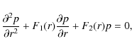
with r the radial coordinate, p the perturbed pressure,
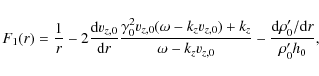
|
(4) |
and
| F2(r) | = | 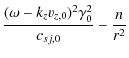
|
|
| (5) |
where
Equation (3) was solved
using the shooting method. This implies integration with a Runge-Kutta
of variable step, from the axis to a given radius far from the jet
boundary, for each pair of temptative values for ![]() and kz.
The boundary conditions on the jet axis are fixed in terms of the
symmetry properties of the perturbation. The roots are found by fixing
a real value of the wavenumber and looking for the roots (complex
frequency) of the boundary condition that states that the amplitude of
the wave must be zero far from the jet. The root-finder used with this
purpose is the Müller method for equations of complex variable (check
Paper II for details). This process of calculation explains the
point-to-point structure of the results shown. In addition, Bessel
functions with complex arguments, which appear as solutions to
Eq. (3), are numerically computed. This is the first time that these kinds of results are systematically
obtained for relativistic, sheared, cylindrical jets.
and kz.
The boundary conditions on the jet axis are fixed in terms of the
symmetry properties of the perturbation. The roots are found by fixing
a real value of the wavenumber and looking for the roots (complex
frequency) of the boundary condition that states that the amplitude of
the wave must be zero far from the jet. The root-finder used with this
purpose is the Müller method for equations of complex variable (check
Paper II for details). This process of calculation explains the
point-to-point structure of the results shown. In addition, Bessel
functions with complex arguments, which appear as solutions to
Eq. (3), are numerically computed. This is the first time that these kinds of results are systematically
obtained for relativistic, sheared, cylindrical jets.
![\begin{figure}
\par\mbox{\includegraphics[clip,angle=0,width=6cm]{13012f1a.ps}\q...
....ps}\quad
\includegraphics[clip,angle=0,width=6cm]{13012f1i.ps} }\end{figure}](/articles/aa/full_html/2010/11/aa13012-09/img36.png)
|
Figure 1: Solutions to the linear problem. Upper panels show the solutions for model B05, central panels show the solutions for model D10, and the bottom panels show the solutions for model B20. The left column displays the pinching modes, the central column shows the helical modes, and the right column shows the elliptic modes. In each of the panels, the upper lines represent the real part of the frequency, whereas the lower lines represent the imaginary part of the frequency, i.e., the growth rate. The surface modes are those with no zeros between the jet axis and its surface, whereas the body modes have one or more zeros in this region. They appear from left to right in the images. |
| Open with DEXTER | |
The results shown in Fig. 1 reveal that the helical and elliptical surface modes dominate the growth rates at the longer wavelengths (low-order modes) for the three models. The plots show that the surface mode is damped at short wavelengths for colder jets (B05 and B20, top and bottom panels) when compared with the hotter jet (D10, central panels). The growth rates tend to decrease from B05 and D10 to B20, i.e., with the Lorentz factor and relativistic Mach number. The resonant modes dominate the solutions at the shorter wavelengths in all the models. Their growth rates are higher than those of the low-order modes. These results coincide with those obtained in Paper II for jets with slab geometry.
We excited several modes for each model (
![]() and
and
![]() ).
In the case of B05, the pinching perturbations excite wavelengths
surrounding the maximum growth rate of the first body mode, of the
second body mode, and the resonant modes, whereas the helical and
elliptical perturbations excite the surface, first body, second body,
and resonant modes. In the case of D10 the pinching perturbations
trigger the surface (at a very low growth rate), first and fourth body
modes, and the helical and elliptical perturbations excite the surface
and fourth and third body modes, respectively. Finally, in the case of
B20, all the perturbations excite the first or second body modes and
the resonant modes, as the surface mode is damped at the low values of
the wave-number (
).
In the case of B05, the pinching perturbations excite wavelengths
surrounding the maximum growth rate of the first body mode, of the
second body mode, and the resonant modes, whereas the helical and
elliptical perturbations excite the surface, first body, second body,
and resonant modes. In the case of D10 the pinching perturbations
trigger the surface (at a very low growth rate), first and fourth body
modes, and the helical and elliptical perturbations excite the surface
and fourth and third body modes, respectively. Finally, in the case of
B20, all the perturbations excite the first or second body modes and
the resonant modes, as the surface mode is damped at the low values of
the wave-number (
![]() for the helical surface mode and
for the helical surface mode and
![]() for
the elliptical surface mode). We can thus anticipate from these results
that the resonant modes may influence the growth of perturbations in
all three cases, but will be more important in the case of pinching and
helical modes in B20, due to their higher relative growth-rates.
for
the elliptical surface mode). We can thus anticipate from these results
that the resonant modes may influence the growth of perturbations in
all three cases, but will be more important in the case of pinching and
helical modes in B20, due to their higher relative growth-rates.
![\begin{figure}
\par\mbox{\includegraphics[clip,angle=0,width=8.8cm]{13012f2a.ps}\quad
\includegraphics[clip,angle=0,width=8.8cm]{13012f2b.ps} }
\end{figure}](/articles/aa/full_html/2010/11/aa13012-09/img41.png)
|
Figure 2: Left panels: pressure perturbation across the jet axis for models B05 ( left panels) and B20 ( right panels) at two different times (t1 and t2 in Fig. 3 for B05 and t1 and t3 for B20), within the linear regime ( upper row) and close to the end of the linear regime ( lower row). Arrows in Fig. 3 indicate these times. Right panels: specific internal energy across the jet axis for models B05 ( left panels) and B20 ( right panels) at the same times. The two lines (solid and dotted) stand for two different positions along the jet axis, at half the grid-size distance to each other, where the cuts are done. Note the change in scale between the upper and lower plots. |
| Open with DEXTER | |
During the linear evolution, the resonant modes are excited either
directly or as harmonics of the longer wavelengths and may grow faster
than the latter, as explained in the previous paragraph. In
Paper II, the authors showed that these modes grow faster in the
shear layer between the jet and the ambient. Thus if the resonant modes
dominate the growth, the largest mode amplitudes are expected towards
the shear layer. The upper panels in Fig. 2
show the typical profiles produced by the growth of resonant modes (see
Figs. 4 and 9 in Paper II) for models B05 (left) and B20 (right).
The radial profile of the perturbations in these jets is clearly
dominated by the resonant modes. However, this does not imply that they
have the highest amplitude in the whole volume of the jet, as revealed
by a Fourier analysis along the jet (not shown here), which shows that
they are in competition with the longer wavelengths, mainly in the case
of B05. Axial profiles of the pressure perturbation (not shown) taken
at
![]() reveal long antisymmetric structures along the jet for model B05,
together with the short scale oscillations, whereas in the case of B20,
the long structures appear to be mainly symmetric (due to the high
growth-rate of the elliptical modes) and short scale oscillations of
comparable amplitude are also visible.
reveal long antisymmetric structures along the jet for model B05,
together with the short scale oscillations, whereas in the case of B20,
the long structures appear to be mainly symmetric (due to the high
growth-rate of the elliptical modes) and short scale oscillations of
comparable amplitude are also visible.
The lower panels in Fig. 2 show the same variables at a later time, close to the end of the linear regime (as defined in Perucho et al. 2004a). The evolution of the pressure perturbation in time is very similar, in both cases, to that shown in Fig. 9 of Paper II, with the larger amplitudes initially showing up in the sheared region. We show, in the right panels of Fig. 2, two cuts of specific internal energy across the jet for both models, at the same times as in the left panels. Both the upper (in the linear regime) and lower (about the end of the linear regime) plots reveal that the resonant modes convert more energy into heat in the shear layer in the case of model B20. Thus, as expected from the linear solutions (see Fig. 1), these modes influence the dynamics of this jet more.
![\begin{figure}
\par\includegraphics[clip,angle=0,width=8.8cm]{13012f3.ps}
\end{figure}](/articles/aa/full_html/2010/11/aa13012-09/img43.png)
|
Figure 3: Evolution of axial momentum in the jets with time. The solid line stands for model B05, the dotted line for model D10 and the dashed line for model B20. Indicated with arrows, the times at which the cuts in Fig. 2 were taken: t1 is the time of first cut for both models, t2 the time of the second cut for B05, and t3 the time of the second cut for B20. |
| Open with DEXTER | |
3.2 Nonlinear regime
In previous works the stability of jets in the nonlinear regime was characterized in terms of mixing and transfer of linear momentum to the ambient medium (Perucho et al. 2004b; and Paper I). Following these criteria, we discuss here the stability of the simulated jets. The axial momentum in the simulated jets is displayed versus time in Fig. 3, normalized to their value at t=0. The longitudinal momentum in the jet is computed by multiplying the actual axial momentum in each cell by the jet mass fraction. During the linear regime, we observe no transfer of linear momentum from the jet to the ambient. This regime is shorter in these simulations than in the 2D ones because the initial amplitudes of the perturbations have been set to be larger with the aim of reducing the computational times. In the nonlinear regime, the plots show a clear trend following the results reported in Paper I: model B05 loses the largest amount of axial momentum and model B20 keeps a large part of it at the end of the simulation. The latter was kept running longer than models B05 and D10 to check that this trend is valid during long times in the nonlinear regime. Model D10 was stopped at an earlier stage than B05 because the time-step became progressively shorter during the nonlinear regime and the simulation demanded too much time to be continued from this point.
![\begin{figure}
\par\mbox{\includegraphics[clip,angle=0,width=8.8cm]{13012f4a.ps}\quad
\includegraphics[clip,angle=0,width=8.8cm]{13012f4b.ps} }
\end{figure}](/articles/aa/full_html/2010/11/aa13012-09/img44.png)
|
Figure 4: Axial cut of Lorentz factor ( left) and jet mass fraction (tracer, right), along the central planes for model B05 at the end of the simulations. The tracer has a value of 1 for the original jet material, 0 for the ambient medium material and values between 0 and 1 in those cells where mixing is present. |
| Open with DEXTER | |
![\begin{figure}
\par\mbox{\includegraphics[clip,angle=0,width=8.8cm]{13012f5a.ps}\quad
\includegraphics[clip,angle=0,width=8.8cm]{13012f5b.ps} }
\end{figure}](/articles/aa/full_html/2010/11/aa13012-09/img45.png)
|
Figure 5: Axial cut of Lorentz factor ( left) and jet mass fraction (tracer, right), along the central planes for model D10 at the end of the simulations. |
| Open with DEXTER | |
![\begin{figure}
\par\mbox{\includegraphics[clip,angle=0,width=8.8cm]{13012f6a.ps}\quad
\includegraphics[clip,angle=0,width=8.8cm]{13012f6b.ps} }
\end{figure}](/articles/aa/full_html/2010/11/aa13012-09/img46.png)
|
Figure 6: Axial cut of Lorentz factor ( left) and jet mass fraction (tracer, right), along the central planes for model B20 at the end of the simulations. |
| Open with DEXTER | |
![\begin{figure}
\par\includegraphics[clip,angle=0,width=18cm]{13012f7.ps}
\end{figure}](/articles/aa/full_html/2010/11/aa13012-09/img48.png)
|
Figure 7:
Transversal cut of Lorentz factor ( left), logarithm of specific internal energy (c2, centre) and jet mass fraction (tracer, right), at
|
| Open with DEXTER | |
Figures 4 (model B05), 5 (D10), and 6
(B20) display axial cuts at the final snapshot in Lorentz factor and
tracer (jet mass fraction) for the three simulations. The maximum
Lorentz factor in the maps of models B05 is
![]() ,
in the maps of model D10 is
,
in the maps of model D10 is
![]() ,
and
,
and
![]() for model B20. Regarding the tracer, white indicates original, unmixed
jet material. From these maps, we see that B05 is completely mixed and
D10 is strongly entrained, although both models keep a central region
with the higher values of this variable, whereas model B20 keeps a
central spine with little or no mixing.
for model B20. Regarding the tracer, white indicates original, unmixed
jet material. From these maps, we see that B05 is completely mixed and
D10 is strongly entrained, although both models keep a central region
with the higher values of this variable, whereas model B20 keeps a
central spine with little or no mixing.
The maps show the effect of the different modes in the structure of the flow and a gradient in the stability of the jets from B05 and D10 to B20, as could be expected from Fig. 3. Although the mixture of growing modes makes it difficult to identify the individual ones, these images allow us to see which wavelenghts dominate the nonlinear regime. Model B05 shows a helical structure with the size of the box that can be attached to the surface mode (see Fig. 1), but also small-scale efficient mixing structures resulting from the growth of the short-wavelength resonant modes. The Fourier transform shows competition among different harmonics, mainly the fundamental mode of the box, followed in amplitude by the first harmonic and a mixture of higher order harmonics, which coincides with the predictions from the linear regime. The rapid disruption of this jet is the consequence of the distortion of the jet surface by the longer wavelengths.
The central spine of model D10 shows a short wavelength (
![]() ), helical structure, which could be identified with the fourth body mode (see Fig. 1),
and, on the same scales, expansions and contractions of the jet, which
could come either from the fourth pinching body mode or from the third
elliptical body mode. These structures are surrounded by a layer where
small-scale mixing occurs. In this region, an
), helical structure, which could be identified with the fourth body mode (see Fig. 1),
and, on the same scales, expansions and contractions of the jet, which
could come either from the fourth pinching body mode or from the third
elliptical body mode. These structures are surrounded by a layer where
small-scale mixing occurs. In this region, an
![]() helical pattern can be seen. This result clearly shows that different
wavelengths may show up at different jet radii, generating a radial
profile, as already shown in Perucho et al. (2006).
The Fourier transform indicates that the highest amplitudes correspond
to the fundamental mode and first harmonic at the end of the linear
regime, followed by high-order harmonics, which keep growing slowly
after the end of the linear regime until saturation of the growth of
the radial velocity and domination of the nonlinear regime in the long
term. The growth rates shown in Fig. 1
agrees with the importance of the third to sixth body modes during the
evolution. However, in contrast to the colder models, the linear
solution does not show small-scale resonances for high-order body
modes, but the resonances occur for those low-order body modes, which
may be the reason for the final disruption of the jet. The structure of
jet D10, with maxima and minima in the Lorentz factor along the axial
directions will make shock waves arise naturally, which may mix the jet
further and eventually disrupt it.
helical pattern can be seen. This result clearly shows that different
wavelengths may show up at different jet radii, generating a radial
profile, as already shown in Perucho et al. (2006).
The Fourier transform indicates that the highest amplitudes correspond
to the fundamental mode and first harmonic at the end of the linear
regime, followed by high-order harmonics, which keep growing slowly
after the end of the linear regime until saturation of the growth of
the radial velocity and domination of the nonlinear regime in the long
term. The growth rates shown in Fig. 1
agrees with the importance of the third to sixth body modes during the
evolution. However, in contrast to the colder models, the linear
solution does not show small-scale resonances for high-order body
modes, but the resonances occur for those low-order body modes, which
may be the reason for the final disruption of the jet. The structure of
jet D10, with maxima and minima in the Lorentz factor along the axial
directions will make shock waves arise naturally, which may mix the jet
further and eventually disrupt it.
![\begin{figure}
\par\includegraphics[clip,angle=0,width=18cm]{13012f8.ps}
\end{figure}](/articles/aa/full_html/2010/11/aa13012-09/img53.png)
|
Figure 8: Mean values of Lorentz factor ( left), logarithm of specific internal energy (c2, centre), and jet mass fraction (tracer, right), averaged along the jet axis for model B05 ( top panels), D10 ( middle panels), and B20 ( bottom panels) at the end of the simulations. Scales on the different panels are fixed to span the interval between the local minima and maxima. |
| Open with DEXTER | |
Model B20 presents a more collimated structure and shows a combination of expansions and contractions plus a helical pattern with the wavelength of the box, corresponding to the first body helical mode. As in model D10, there is a thick mixing layer surrounding the jet core. The Fourier transform also shows that the fundamental mode of the box (corresponding to the helical first body mode) dominates during the linear regime, but also the fast growth of the higher harmonics, which, like before, surpass the amplitude of the long wavelength during the time interval between the end of the linear regime and the saturation of the radial velocity. This competition between the longest wavelength and the shorter ones can be deduced from Fig. 1. In the case of model B20, the structure at the end of the simulation points towards further mixing, although this jet has a higher Lorentz factor and a more uniform structure than D10 at the end of the simulation.
Figure 7 shows transversal cuts at half way through the grid at the end of the simulation. The figure shows the final distorted structure and turbulent mixing in all three models. The top panels show that model B05 is completely mixed (see the tracer in the right panel), whereas D10 and B20 still keep a fast, unmixed spine, which is larger in the latter. B20 shows a hot shear layer including the slower, outer regions of this unmixed core, contrary to D10 and B05, where the temperature decreases outwards. The centroid of model B20 is displaced left and down from the centre of coordinates, indicating helical motion in competition with the elliptical modes, responsible for the oblique elongation of the jet section. There are hints of a similar deformation in model D10, but no significant displacement of the centre of the jet is detected in this case. This may be because the dominating helical structure is given by a short wavelength mode, which only generates small displacements (Hardee 2000). Also model B05 shows an elongation (vertical in this cut), but any hints of regular structure have been smeared out by the mixing and disruption of the original flow. It is also difficult to assess whether the axis of the jet is displaced by helical modes; this can be better observed in the axial cuts.
To have a global view of the parameters along the jet axis, we show in Fig. 8
mean axial values of different physical parameters for the three models
at the end of each simulation. In these panels, the displacement of the
axis due to the helical modes is promediated and thus we always find
the centre of the jets around their original position. The left panels
display the Lorentz factor and show barely relativistic motion for
model B05, with maximum Lorentz factor
![]() ,
as compared to models D10 (
,
as compared to models D10 (
![]() )
and B20 (
)
and B20 (
![]() ).
The central panels show the logarithm of the specific internal energy
and show the same behaviour as observed in the 2D simulations of
Papers I and II: the generation of a hot shear layer around
the core in those models in which the resonant modes already dominate
during the linear regime (model B20), due to the strong dissipation of
kinetic into internal energy in this area, when the resonant modes
achieve the nonlinear regime. The right panels show the tracer, which
represents the percentage of initial jet material in a cell. In the
case of model B05, the whole jet is mixed with the ambient medium, as
indicated by the maximum original jet mass fraction in a cell (
).
The central panels show the logarithm of the specific internal energy
and show the same behaviour as observed in the 2D simulations of
Papers I and II: the generation of a hot shear layer around
the core in those models in which the resonant modes already dominate
during the linear regime (model B20), due to the strong dissipation of
kinetic into internal energy in this area, when the resonant modes
achieve the nonlinear regime. The right panels show the tracer, which
represents the percentage of initial jet material in a cell. In the
case of model B05, the whole jet is mixed with the ambient medium, as
indicated by the maximum original jet mass fraction in a cell (![]() 21%), model D10 shows some mixing down to the axis (with maximum mean jet mass fraction
21%), model D10 shows some mixing down to the axis (with maximum mean jet mass fraction ![]()
![]() on the jet axis), whereas in model B20 the central spine remains
unmixed and collimated. Regarding the width of the mixing layer, we
observe that model B05 presents the wider mixing region, whereas D10
has the thinnest one. However, if we consider that D10 was stopped much
before the other models and that, from Fig. 3
the expected evolution is close to that of B05, we expect that the
mixing layer of D10 after some time should be wider than that of B20.
on the jet axis), whereas in model B20 the central spine remains
unmixed and collimated. Regarding the width of the mixing layer, we
observe that model B05 presents the wider mixing region, whereas D10
has the thinnest one. However, if we consider that D10 was stopped much
before the other models and that, from Fig. 3
the expected evolution is close to that of B05, we expect that the
mixing layer of D10 after some time should be wider than that of B20.
4 Discussion
4.1 Effects of the numerical resolution
In Perucho et al. (2004a) it was shown
that the resolution used in the simulations is crucial to reproducing
the linear growth rates of the modes in the linear regime. In
particular, the resolution may affect the evolution of the shortest
(resonant) modes, which can be damped by numerical viscosity, and also
have implications in the nonlinear regime with respect to, e.g.,
mixing. Thus, we performed several tests to check the influence of the
resolution on our results. First, 2D numerical tests of models B05 and
B20 were performed in which we used the same resolution as in the 3D
simulations, and compared them with the results obtained for
cylindrical jets in 2D (see Appendix B in Paper I). In these
low-resolution simulations, we only excited the pinching modes. In the
case of B05, the disruption of the 2D jet is faster, both in the
low-resolution and the high-resolution cases, than in the 3D case,
because long-wavelength modes have the largest amplitudes at the end of
the linear regime. In 3D, the growth of short-wavelength modes (helical
and/or elliptic) may be responsible for the slower mixing process.
Between the 2D simulations, the low-resolution one shows a slower
mixing and momentum transfer to the ambient, implying that the
resolution affects this process, as expected. In model B20, we identify
the effects of resonant modes also in the low-resolution 2D simulation,
which result in a slow transfer of axial momentum from the jet to the
environment during more than
![]() code time units. However, the amplitude of these resonant modes at the
end of the linear regime is less than in the high-resolution case. This
translates into a decrease in the Lorentz factor down to the jet axis
and more transfer of momentum from the jet to the ambient in the
low-resolution case, around an equivalent time to what is reached by
the high-resolution simulation. We continued the low-resolution
simulation further and found that the oscillations in the amplitude of
all the (excited) modes close to their limit of growth (see Perucho et al. 2004b; and Paper I) end up in a long wavelength disrupting the flow. This occurs at time
code time units. However, the amplitude of these resonant modes at the
end of the linear regime is less than in the high-resolution case. This
translates into a decrease in the Lorentz factor down to the jet axis
and more transfer of momentum from the jet to the ambient in the
low-resolution case, around an equivalent time to what is reached by
the high-resolution simulation. We continued the low-resolution
simulation further and found that the oscillations in the amplitude of
all the (excited) modes close to their limit of growth (see Perucho et al. 2004b; and Paper I) end up in a long wavelength disrupting the flow. This occurs at time
![]() ,
which, for a flow with radius, e.g.,
,
which, for a flow with radius, e.g.,
![]() propagating close to the speed of light, implies covering a distance greater than
propagating close to the speed of light, implies covering a distance greater than
![]() before disruption. We should expect that higher resolution would allow
for an undamped growth of resonant modes, thus making these jets even
more stable.
before disruption. We should expect that higher resolution would allow
for an undamped growth of resonant modes, thus making these jets even
more stable.
In addition, we performed a 3D simulation of model B05 with twice the
resolution used here. In this case, we would expect a faster growth of
the resonant modes already detected in the 3D low-resolution
simulation. This simulation was run in the linear and postlinear regime
only during ![]()
![]() code time units due to the computational time limitations. The results
confirm the previous statements: the (helical or elliptic) resonant
modes grow faster and make the mixing of this jet slower (up to the
moment in which we stopped the simulation) when higher resolution is
used.
code time units due to the computational time limitations. The results
confirm the previous statements: the (helical or elliptic) resonant
modes grow faster and make the mixing of this jet slower (up to the
moment in which we stopped the simulation) when higher resolution is
used.
In conclusion, the low resolution may quantitatively affect the results, damping the growth of the resonant modes and also reducing the mixing and momentum transfer rates, but the results presented here are qualitatively equivalent to those obtained in 2D with higher resolution.
4.2 Implications for jet collimation
The results are thus consistent with those of Papers I and II, where the authors showed that the growth of resonant modes in sheared jets can influence the evolution of relativistic flows, by generating small-scale mixing in the shear layer and avoiding the generation of large scale nonlinear structures that may disrupt the whole jet. This result could be important for our understanding of the properties of stability of relativistic outflows on the kiloparsec scales. Even though the Lorentz factors of both FRI and FRII jets appear to be similar on the parsec scales (Celotti & Ghisellini 2008; Giovannini et al. 2001), the present paradigm of FRI jets (Laing 1996; Bicknell 1984; Laing 1993) states that, on kiloparsec scales, these jets are decelerated by entrainment of gas and their properties become different from those of FRII jets on these scales. Two main processes have been invoked to explain the entrainment in jets and studied in the literature: (i) entrainment through mixing in a turbulent shear layer between the jet and the medium (De Young 1986; Bicknell 1994; De Young 1993); and (ii) entrainment from stellar mass losses (Bowman et al. 1996; Laing & Bridle 2002; Komissarov 1994). Recent numerical simulations deal with this last process (Perucho et al., in preparation). Concerning the process of entrainment through a turbulent shear layer, Perucho & Martí (2007) showed, via a 2D axisymmetric simulation, that a recollimation shock in a light jet, in reaction to a steep interstellar density and pressure gradients, may trigger nonlinear perturbations that lead to jet mixing and disruption with the external medium. Later, Rossi et al. (2008) obtained a similar result in 3D for a homogeneous ambient medium, where the shock is induced by an overpressured cocoon. Also Meliani et al. (2008) studied the influence of a discontinuous jump in the external density gas on the jet disruption in hybrid FRI/FRII sources, where the jet and counterjet present different morphology, and this is adscribed to such environmental irregularities.
Regardless of the origin of the deceleration, the Lorentz factors in FRI jets after
![]() may
already be small enough to favor the growth of KH modes, triggering the
mixing process. In the context of the FRI/FRII dichotomy, the evolution
of the KH instability can thus be seen as a consequence of this
dichotomy and a cause of the kiloparsec-scale morphology of the two
types of jets, where in one case the growth of the KH modes favor
mixing and in the other may favor further collimation. In the case of
FRII jets, the strong recollimation shocks or strong entrainment
discussed in the previous paragraph do not seem to happen.
Nevertheless, they do show knotty structure due to oscillations around
pressure equilibrium with the ambient medium or to travelling
perturbations. In both cases and also if perturbations are induced by
irregularities in the surrounding medium (typically the backflow or
cocoon, e.g., Mizuta et al. 2010), these could couple to KH instabilities (e.g., Agudo et al. 2001).
Despite this, the FRII jets seem to be collimated up to distances of
hundreds of kiloparsecs. To our knowledge, there are only two proposed
mechanisms that could keep jets collimated: (i) the action of magnetic
fields, a mechanism which does not work if the jets are not
magnetically dominated, as is thought to be the case at kiloparsec
scales (see, e.g., Sikora et al. 2005); or
(ii) by inertial confinement, which seems not to be possible within the
low-density cavities with decreasing pressure (see, e.g. simulations by
Scheck et al. 2002; Perucho & Martí 2007),
where large-scale jets propagate. We propose here a third mechanism,
purely hydrodynamical, that prevents the decollimation of relativistic
jets, based on the growth of resonant modes.
may
already be small enough to favor the growth of KH modes, triggering the
mixing process. In the context of the FRI/FRII dichotomy, the evolution
of the KH instability can thus be seen as a consequence of this
dichotomy and a cause of the kiloparsec-scale morphology of the two
types of jets, where in one case the growth of the KH modes favor
mixing and in the other may favor further collimation. In the case of
FRII jets, the strong recollimation shocks or strong entrainment
discussed in the previous paragraph do not seem to happen.
Nevertheless, they do show knotty structure due to oscillations around
pressure equilibrium with the ambient medium or to travelling
perturbations. In both cases and also if perturbations are induced by
irregularities in the surrounding medium (typically the backflow or
cocoon, e.g., Mizuta et al. 2010), these could couple to KH instabilities (e.g., Agudo et al. 2001).
Despite this, the FRII jets seem to be collimated up to distances of
hundreds of kiloparsecs. To our knowledge, there are only two proposed
mechanisms that could keep jets collimated: (i) the action of magnetic
fields, a mechanism which does not work if the jets are not
magnetically dominated, as is thought to be the case at kiloparsec
scales (see, e.g., Sikora et al. 2005); or
(ii) by inertial confinement, which seems not to be possible within the
low-density cavities with decreasing pressure (see, e.g. simulations by
Scheck et al. 2002; Perucho & Martí 2007),
where large-scale jets propagate. We propose here a third mechanism,
purely hydrodynamical, that prevents the decollimation of relativistic
jets, based on the growth of resonant modes.
According to our results (Papers I and II and this
work), this mechanism is more effective in jets with larger flow
Lorentz factors, but also depends on the initial width of the shear
layer and on the temperature of the jet. Solutions to the linear
perturbation problem in a sheared, relativistic jet show that, if the
jet is separated from the ambient by a pure contact discontinuity
(vortex sheet) or by a very thick shear layer (>
![]() )
)![]() ,
the resonances do not develop, thus leading to unstable configurations
in which the jets can be disrupted by the growth of instabilities. The
same solutions, along with numerical simulations, show that the
resonances grow faster in colder jets, at a constant Lorentz factor. In
addition, it was shown in previous works that lower density ratios
between the jet and the ambient medium may also lead to the disruption
of the jet by the growth of instabilities.
,
the resonances do not develop, thus leading to unstable configurations
in which the jets can be disrupted by the growth of instabilities. The
same solutions, along with numerical simulations, show that the
resonances grow faster in colder jets, at a constant Lorentz factor. In
addition, it was shown in previous works that lower density ratios
between the jet and the ambient medium may also lead to the disruption
of the jet by the growth of instabilities.
We know at least one case in which a jet classified as an FRII (0836+710, Hummel et al. 1992) for its luminosity, seems to be disrupted by the growth of instabilities on the kiloparsec scales. This could be assigned to the growth of instabilities (Perucho & Lobanov 2007). Perhaps in this case, the conditions in the jet (e.g., thickness of the shear layer or physical parameters in the jet) are such that resonant modes are not excited.
One observational feature of the growth of these modes would be the edge brightening of jets, which should mainly occur in FRII jets. Possible evidence of hot shear layers is given by Swain et al. (1998), who show that the jets in the FRII radio galaxy 3C 353 have some transversal structure with higher radio-emission towards the boundaries of the jet. These hot shear layers could be generated by the growth of resonant modes as shown by our simulations. In addition, Kadler et al. (2008) suggest the growth of resonant modes as the mechanism that provides the long-term stability of the jet in the FRII radio galaxy 3C 111. A possible test for this hypothesis would be to check the transversal structure in this and other FRII jets seeking enhanced emission at the jet boundaries. From the point of view of particle acceleration, the hot and turbulent (down to numerical resolution) mixing layers produced by the resonant modes may be sites of efficient acceleration of non-thermal particles (e.g., Stawarz & Ostrowski 2002; Aloy & Mimica 2008).
5 Conclusions
In this work, we presented the first solutions of the linear problem for 3D sheared relativistic flows. Following this result, we presented numerical simulations of the growth of KH instability modes from the linear to the nonlinear regimes, for three selected relativistic jet models. These numerical simulations were performed with the new high-resolution shock-capturing 3D RHD code Ratpenat, which was parallelized using a hybrid scheme with OMP and MPI processes. The simulations of jets in the typical stability regions of the space of parameters (Paper I) have confirmed previous results obtained in the 2D approximation. We proved that under certain conditions, the appearance of the shear-layer resonant modes of KH instability has important consequences for the stability of relativistic jets. In particular, the implications for the collimation of FRII jets were discussed. We also show, as a by-product of our simulations, that the development of different modes with a variety of wavelengths may induce rich transversal structure in jets, with shorter modes showing up in the central regions of the jet and longer ones dominating the structure in the mixing layer. In this respect, we confirm the results obtained in Perucho et al. (2006).
Future work along this line will consider the extension of our study in both the linear and nonlinear regime by means of simulations with higher resolution to a wider sample of jet parameters, including magnetic fields and a more realistic equation of state.
AcknowledgementsM.P. acknowledges support from a postdoctoral fellowship of the ``Generalitat Valenciana'' (``Beca Postdoctoral d'Excellència'') and a ``Juan de la Cierva'' contract of the Spanish ``Ministerio de Ciencia y Tecnología''. M.P. and J.M.M. acknowledge support by the Spanish ``Ministerio de Educación y Ciencia'' and the European Fund for Regional Development through grants AYA2007-67627-C03-01 and AYA2007-67752-C03-02 and Consolider-Ingenio 2010, Ref. 20811. M.H. acknowledges support by Polish MNiSW grant 92/N-ASTROSIM/2008/0. M.P. benefitted from the HPC-Europa pogramme. The authors acknowledge the BSC. We thank E. Ros for criticism and comments to the original paper.
References
- Agudo, I., Gómez, J. L., Martí, J. M., et al. 2001, ApJ, 549, L183 [NASA ADS] [CrossRef] [Google Scholar]
- Aloy, M. A., & Mimica, P. 2008, ApJ, 681, 84 [NASA ADS] [CrossRef] [Google Scholar]
- Aloy, M. A., Ibáñez, J. M., Martí, J. M., & Müller, E. 1999, ApJS, 122, 151 [NASA ADS] [CrossRef] [Google Scholar]
- Blandford, R. D., & Pringle, J. E. 1976, MNRAS, 176, 443 [NASA ADS] [CrossRef] [Google Scholar]
- Bicknell, G. V. 1984, ApJ, 286, 68 [NASA ADS] [CrossRef] [Google Scholar]
- Bicknell, G. V. 1994, ApJ, 422, 542 [NASA ADS] [CrossRef] [Google Scholar]
- Bodo, G., Massaglia, S., Ferrari, A., & Trussoni, E. 1994, A&A, 283, 655 [NASA ADS] [Google Scholar]
- Bowman, M., Leahy, J. P., & Komissarov, S. S. 1996, MNRAS, 279, 899 [NASA ADS] [CrossRef] [Google Scholar]
- Carilli, C. L., & Barthel, P. D. 1996, A&ARv, 7, 1 [NASA ADS] [CrossRef] [EDP Sciences] [Google Scholar]
- Celotti, A., & Ghisellini, G. 2008, MNRAS, 385, 283 [NASA ADS] [CrossRef] [Google Scholar]
- De Young, D. S. 1986, ApJ, 307, 62 [NASA ADS] [CrossRef] [Google Scholar]
- De Young, D. S. 1993, ApJ, 405, L13 [NASA ADS] [CrossRef] [Google Scholar]
- Fanaroff, B. L., & Riley, J. M. 1974, MNRAS, 167, 31 [NASA ADS] [CrossRef] [Google Scholar]
- Ferrari, A., Trussoni, E., & Zaninetti, L. 1978, A&A, 64, 43 [NASA ADS] [Google Scholar]
- Giovannini, G., Cotton, W. D., Feretti, L., Lara, L., & Venturi, T. 2001, ApJ, 552, 508 [NASA ADS] [CrossRef] [Google Scholar]
- Hanasz, M. 1995, Ph.D. Thesis, Nicholas Copernicus University, Torun [Google Scholar]
- Hanasz, M. 1997, in Relativistic jets in AGNs, Proc. Int. Conf. held in Cracow (Poland), ed. M. Ostrowski, M. Sikora, G. Madejski, & M. Begelman, 85 [Google Scholar]
- Hardee, P. E. 1979, ApJ, 234, 47 [NASA ADS] [CrossRef] [Google Scholar]
- Hardee, P. E. 2000, ApJ, 533, 176 [NASA ADS] [CrossRef] [Google Scholar]
- Hardee, P. E. 2006, in Relativistic Jets: The Common Physics of AGN, Microquasars and Gamma-Ray Bursts, ed. P. A. Hughes, & J. N. Bregman, AIP Conf. Proc., 856, 57 [Google Scholar]
- Hardee, P. E. 2008, ApJ, 664, 26 [Google Scholar]
- Hardee, P. E., Rosen, A., Hughes, P. A., & Duncan, G. C. 1998, ApJ, 500, 559 [Google Scholar]
- Hardee, P. E., Hughes, P. A., Rosen, A., & Gomez, E. A. 2001, ApJ, 555, 744 [NASA ADS] [CrossRef] [Google Scholar]
- Hummel, C. A., Muxlow, T. W. B., Krichbaum, T. P., et al. 1992, A&A, 266, 93 [NASA ADS] [Google Scholar]
- Kadler, M., Ros, E., Perucho, M., et al. 2008, ApJ, 680, 867 [NASA ADS] [CrossRef] [Google Scholar]
- Komissarov, S. S. 1994, MNRAS, 269, 394 [NASA ADS] [CrossRef] [Google Scholar]
- Laing R. A. 1993, in Space Telescope Science Institute Symposium Series, ed. D. Burgarella, M. Livio, & C. P. ODea, Astrophysical Jets, STScI, Baltimore (Cambridge: Cambridge Univ. Press), 95 [Google Scholar]
- Laing, R. A. 1996, in Energy Transport in Radio Galaxies and Quasars, ed. P. E. Hardee, A. H. Bridle, & J. A. Zesus (San Francisco: ASP), ASP Conf. Ser. 100, 241 (Dordrecht: Kluwer) IAU Symp. Proc., 175, 147 [Google Scholar]
- Laing, R. A., & Bridle, A. H. 2002, MNRAS, 336, 328 [NASA ADS] [CrossRef] [Google Scholar]
- Martí, J. M., Müller, E., Font, J. A., Ibáñez, J. M., & Marquina, A. 1997, ApJ, 479, 151 [NASA ADS] [CrossRef] [Google Scholar]
- Meliani, Z., Keppens, R., & Giacomazzo, B. 2008, A&A, 491, 321 [NASA ADS] [CrossRef] [EDP Sciences] [Google Scholar]
- Mizuno, Y., Hardee, P. E., & Nishikawa, K.-I. 2007, ApJ, 662, 835 [NASA ADS] [CrossRef] [Google Scholar]
- Mizuta, A., Kino, M., & Nagakura, H. 2010, ApJ, 709, L83 [NASA ADS] [CrossRef] [Google Scholar]
- Perucho, M., & Lobanov, A. P. 2007, A&A, 469, L23 [NASA ADS] [CrossRef] [EDP Sciences] [Google Scholar]
- Perucho, M., & Martí, J. M. 2007, MNRAS, 382, 526 [NASA ADS] [CrossRef] [Google Scholar]
- Perucho, M., Hanasz, M., Martí, J. M., & Sol, H. 2004a, A&A, 427, 415 [NASA ADS] [CrossRef] [EDP Sciences] [Google Scholar]
- Perucho, M., Martí, J. M., & Hanasz, M. 2004b, A&A, 427, 431 [NASA ADS] [CrossRef] [EDP Sciences] [Google Scholar]
- Perucho, M., Martí, J. M., & Hanasz, M. 2005, A&A, 443, 863 (Paper I) [NASA ADS] [CrossRef] [EDP Sciences] [Google Scholar]
- Perucho, M., Lobanov, A. P., Martí, J. M., & Hardee, P. E. 2006, A&A, 456, 493 [NASA ADS] [CrossRef] [EDP Sciences] [Google Scholar]
- Perucho, M., Hanasz, M., Martí, J. M., & Miralles, J. A. 2007, Phys. Rev. E, 75, 056312 (Paper II) [NASA ADS] [CrossRef] [Google Scholar]
- Rosen, A., Hughes, P. A., Duncan, G. C., & Hardee, P. E. 1999, ApJ, 516, 729 [NASA ADS] [CrossRef] [Google Scholar]
- Rossi, P., Mignone, A., Bodo, G., Massaglia, S., & Ferrari, A. 2008, A&A, 488, 795 [NASA ADS] [CrossRef] [EDP Sciences] [Google Scholar]
- Scheck L., Aloy, M. A., Martí, J. M., Gómez, J. L., & Müller, E. 2002, MNRAS, 331, 615 [NASA ADS] [CrossRef] [Google Scholar]
- Sikora, M., Begelman, M. C., Madejski, G. M., & Lasota, J.-P. 2005, ApJ, 625, 72 [NASA ADS] [CrossRef] [Google Scholar]
- Stawarz, ▯., & Ostrowski, M. 2002, ApJ, 578, 763 [NASA ADS] [CrossRef] [Google Scholar]
- Swain, M. R., Bridle, A. H., & Baum, S. A. 1998, ApJ, 508, L29 [NASA ADS] [CrossRef] [Google Scholar]
- Turland, B. D., & Scheuer, P. A. G. 1976, MNRAS, 176, 421 [NASA ADS] [Google Scholar]
- Urpin, V. 2002, A&A, 385, 14 [NASA ADS] [CrossRef] [EDP Sciences] [Google Scholar]
Footnotes
- ...
 )
)![[*]](/icons/foot_motif.png)
- Taking the jet radius as the distance where the velocity is half that in the spine, typically
 0.5 c.
All Tables
Table 1: Parameters of the simulations discussed in this paper.
All Figures
|
|
Figure 1: Solutions to the linear problem. Upper panels show the solutions for model B05, central panels show the solutions for model D10, and the bottom panels show the solutions for model B20. The left column displays the pinching modes, the central column shows the helical modes, and the right column shows the elliptic modes. In each of the panels, the upper lines represent the real part of the frequency, whereas the lower lines represent the imaginary part of the frequency, i.e., the growth rate. The surface modes are those with no zeros between the jet axis and its surface, whereas the body modes have one or more zeros in this region. They appear from left to right in the images. |
| Open with DEXTER | |
| In the text | |
|
|
Figure 2: Left panels: pressure perturbation across the jet axis for models B05 ( left panels) and B20 ( right panels) at two different times (t1 and t2 in Fig. 3 for B05 and t1 and t3 for B20), within the linear regime ( upper row) and close to the end of the linear regime ( lower row). Arrows in Fig. 3 indicate these times. Right panels: specific internal energy across the jet axis for models B05 ( left panels) and B20 ( right panels) at the same times. The two lines (solid and dotted) stand for two different positions along the jet axis, at half the grid-size distance to each other, where the cuts are done. Note the change in scale between the upper and lower plots. |
| Open with DEXTER | |
| In the text | |
|
|
Figure 3: Evolution of axial momentum in the jets with time. The solid line stands for model B05, the dotted line for model D10 and the dashed line for model B20. Indicated with arrows, the times at which the cuts in Fig. 2 were taken: t1 is the time of first cut for both models, t2 the time of the second cut for B05, and t3 the time of the second cut for B20. |
| Open with DEXTER | |
| In the text | |
|
|
Figure 4: Axial cut of Lorentz factor ( left) and jet mass fraction (tracer, right), along the central planes for model B05 at the end of the simulations. The tracer has a value of 1 for the original jet material, 0 for the ambient medium material and values between 0 and 1 in those cells where mixing is present. |
| Open with DEXTER | |
| In the text | |
|
|
Figure 5: Axial cut of Lorentz factor ( left) and jet mass fraction (tracer, right), along the central planes for model D10 at the end of the simulations. |
| Open with DEXTER | |
| In the text | |
|
|
Figure 6: Axial cut of Lorentz factor ( left) and jet mass fraction (tracer, right), along the central planes for model B20 at the end of the simulations. |
| Open with DEXTER | |
| In the text | |
|
|
Figure 7:
Transversal cut of Lorentz factor ( left), logarithm of specific internal energy (c2, centre) and jet mass fraction (tracer, right), at
|
| Open with DEXTER | |
| In the text | |
|
|
Figure 8: Mean values of Lorentz factor ( left), logarithm of specific internal energy (c2, centre), and jet mass fraction (tracer, right), averaged along the jet axis for model B05 ( top panels), D10 ( middle panels), and B20 ( bottom panels) at the end of the simulations. Scales on the different panels are fixed to span the interval between the local minima and maxima. |
| Open with DEXTER | |
| In the text | |
Copyright ESO 2010
Current usage metrics show cumulative count of Article Views (full-text article views including HTML views, PDF and ePub downloads, according to the available data) and Abstracts Views on Vision4Press platform.
Data correspond to usage on the plateform after 2015. The current usage metrics is available 48-96 hours after online publication and is updated daily on week days.
Initial download of the metrics may take a while.