| Issue |
A&A
Volume 518, July-August 2010
Herschel: the first science highlights
|
|
|---|---|---|
| Article Number | A45 | |
| Number of page(s) | 10 | |
| Section | Interstellar and circumstellar matter | |
| DOI | https://doi.org/10.1051/0004-6361/201014510 | |
| Published online | 01 September 2010 | |
The CO luminosity and CO-H conversion factor of diffuse ISM:
does CO emission trace dense molecular gas?
conversion factor of diffuse ISM:
does CO emission trace dense molecular gas?![[*]](/icons/foot_motif.png)
H. S. Liszt1 - J. Pety2,3 - R. Lucas4
1 - National Radio Astronomy Observatory, 520 Edgemont Road, VA
22903-2475 Charlottesville, USA
2 - Institut de Radioastronomie Millimétrique, 300 rue de la Piscine,
38406 Saint Martin d'Hères, France
3 - Obs. de Paris, 61 av. de l'Observatoire, 75014 Paris, France
4 - Al-MA, Avda. Apoquindo 3846 Piso 19, Edificio Alsacia, Las Condes,
Santiago, Chile
Received 26 March 2010 / Accepted 8 May 2010
Abstract
Aims. We wish to separate and quantify the CO
luminosity and CO-
![]() conversion factor applicable to diffuse but partially-molecular ISM
when
conversion factor applicable to diffuse but partially-molecular ISM
when ![]() and CO are present but C+ is the dominant form
of gas-phase carbon.
and CO are present but C+ is the dominant form
of gas-phase carbon.
Methods. We discuss galactic lines of sight observed
in ![]() ,
,
![]() and
CO where CO emission is present but the intervening clouds are diffuse
(locally
and
CO where CO emission is present but the intervening clouds are diffuse
(locally ![]()
![]() mag) with
relatively small CO column densities
mag) with
relatively small CO column densities ![]() .
We separate the atomic and molecular fractions statistically using EB-V
as a gauge of the total gas column density and compare
.
We separate the atomic and molecular fractions statistically using EB-V
as a gauge of the total gas column density and compare ![]() to the observed CO brightness.
to the observed CO brightness.
Results. Although there are ![]() -bearing
regions where CO emission is too faint to be detected, the mean ratio
of integrated CO brightness to
-bearing
regions where CO emission is too faint to be detected, the mean ratio
of integrated CO brightness to ![]() for diffuse ISM does not differ from the usual value of 1
for diffuse ISM does not differ from the usual value of 1
![]() of integrated CO brightness per
of integrated CO brightness per ![]()
![]()
![]() .
Moreover, the luminosity of diffuse CO viewed perpendicular to the
galactic plane is 2/3 that seen at the Solar galactic radius in surveys
of CO emission near the galactic plane.
.
Moreover, the luminosity of diffuse CO viewed perpendicular to the
galactic plane is 2/3 that seen at the Solar galactic radius in surveys
of CO emission near the galactic plane.
Conclusions. Commonality of the CO-
![]() conversion factors in diffuse and dark clouds can be understood from
considerations of radiative transfer and CO chemistry. There is
unavoidable confusion between CO emission from diffuse and dark gas and
misattribution of CO emission from diffuse to dark or giant molecular
clouds. The character of the ISM is different from what has been
believed if CO and
conversion factors in diffuse and dark clouds can be understood from
considerations of radiative transfer and CO chemistry. There is
unavoidable confusion between CO emission from diffuse and dark gas and
misattribution of CO emission from diffuse to dark or giant molecular
clouds. The character of the ISM is different from what has been
believed if CO and ![]() that have been attributed to molecular clouds on the verge of star
formation are actually in more tenuous, gravitationally-unbound diffuse
gas.
that have been attributed to molecular clouds on the verge of star
formation are actually in more tenuous, gravitationally-unbound diffuse
gas.
Key words: ISM: molecules - ISM: clouds
1 Introduction
It is a truism that sky maps of CO emission are understood as uniquely
tracing the Galaxy's molecular clouds, dense, cold strongly-shielded
regions where the hydrogen is predominantly molecular and the dominant
form
of gas phase carbon is CO. Moreover, CO emission plays an
especially important role in ISM studies as the tracer of cold
molecular
hydrogen through the use of the so-called CO-
![]() conversion factor which
directly scales the integrated
conversion factor which
directly scales the integrated ![]() J=1-0 brightness
J=1-0 brightness ![]() to
to
![]() column density
column density ![]() .
This deceptively simple conversion
is critically important to determining molecular and total gas column
densities and so to understanding the most basic properties of star
formation (Bothwell
et al. 2009; Bigiel et al. 2008; Leroy
et al. 2008), the origins of galactic dust
emission (Draine et al. 2007),
and other such fundamentals.
.
This deceptively simple conversion
is critically important to determining molecular and total gas column
densities and so to understanding the most basic properties of star
formation (Bothwell
et al. 2009; Bigiel et al. 2008; Leroy
et al. 2008), the origins of galactic dust
emission (Draine et al. 2007),
and other such fundamentals.
Yet, it is increasingly recognized that CO emission is present
along lines
of sight lacking high extinction or large molecular column densities
(Liszt & Lucas
1998). It is also the case that some very opaque lines
of sight showing CO emission are comprised entirely of diffuse material
and
![]() -bearing
diffuse clouds (McCall
et al. 2002): a discussion of
such a line of sight from our own work is described in
Appendix A
here. Even in canonical dark clouds like Taurus, detailed
high-resolution
mapping of the CO emission (Goldsmith
et al. 2008) reveals that much of it
originates in relatively weakly-shielded gas where
-bearing
diffuse clouds (McCall
et al. 2002): a discussion of
such a line of sight from our own work is described in
Appendix A
here. Even in canonical dark clouds like Taurus, detailed
high-resolution
mapping of the CO emission (Goldsmith
et al. 2008) reveals that much of it
originates in relatively weakly-shielded gas where ![]() is strongly
enhanced through isotopic fractionation, implying that the
dominant form of gas phase carbon must be C+ (Watson et al. 1976).
is strongly
enhanced through isotopic fractionation, implying that the
dominant form of gas phase carbon must be C+ (Watson et al. 1976).
![\begin{figure}
\par\includegraphics[height=8cm,clip]{14510f1.eps} \vspace*{-2.5mm}
\end{figure}](/articles/aa/full_html/2010/10/aa14510-10/img25.png)
|
Figure 1:
Atomic and molecular absorption and emission vs. total reddening.
Left: Integrated VLA |
| Open with DEXTER | |
Conversely, it is also the case that molecular gas is detected in the
local
ISM even when CO emission is not. Lines of sight with ![]() ,
,
![]() have
long been detectable in surveys of uv
absorption (Sheffer
et al. 2008; Burgh et al. 2007; Sonnentrucker
et al. 2007; Sheffer et al. 2007),
with expected integrated
CO brightnesses as low as
have
long been detectable in surveys of uv
absorption (Sheffer
et al. 2008; Burgh et al. 2007; Sonnentrucker
et al. 2007; Sheffer et al. 2007),
with expected integrated
CO brightnesses as low as ![]() (Liszt 2007b). And, as
discussed here, mm-wave
(Liszt 2007b). And, as
discussed here, mm-wave ![]() and CO absorption from clouds with
and CO absorption from clouds with ![]() are also more common than CO emission along the same lines of
sight (see Liszt & Lucas 2000;
Lucas
& Liszt 1996, and Appendix A).
are also more common than CO emission along the same lines of
sight (see Liszt & Lucas 2000;
Lucas
& Liszt 1996, and Appendix A).
Thus we are led to ask two questions that are of particular
importance to
the use of CO emission as a molecular gas tracer. First, where and how
does the observed local CO luminosity really originate? Second, how
completely is the molecular material represented by CO emission? The
approach we take to address these issues is based on radiofrequency
surveys
of ![]() ,
,
![]() and
CO absorption and emission along lines of
sight through the Galaxy toward extragalactic background sources. By
combining 1) measurements of extinction (constraining the total gas
column
density); 2) measurements of
and
CO absorption and emission along lines of
sight through the Galaxy toward extragalactic background sources. By
combining 1) measurements of extinction (constraining the total gas
column
density); 2) measurements of ![]() absorption (to determine the gas column
of atomic hydrogen); 3) the strength of
absorption (to determine the gas column
of atomic hydrogen); 3) the strength of ![]() absorption (tracing
absorption (tracing ![]() directly) and 4) the integrated CO J=1-0 brightness
directly) and 4) the integrated CO J=1-0 brightness
![]() ,
we relate
,
we relate ![]() to
to ![]() along sightlines where we have previously shown that the
intervening gas is diffuse, neither dark nor dense, and the CO column
densities are relatively small. The results are somewhat surprising:
although there is much variability, the mean CO brightness per
along sightlines where we have previously shown that the
intervening gas is diffuse, neither dark nor dense, and the CO column
densities are relatively small. The results are somewhat surprising:
although there is much variability, the mean CO brightness per ![]() -molecule
-molecule
![]() /
/
![]() ,
i.e. the CO-
,
i.e. the CO-
![]() conversion factor, does not differ between
diffuse and fully molecular clouds. Although this was
phenomenologically
inferred long ago, the physical basis for it is now better understood
in
terms of the radiative transfer and chemistry of
conversion factor, does not differ between
diffuse and fully molecular clouds. Although this was
phenomenologically
inferred long ago, the physical basis for it is now better understood
in
terms of the radiative transfer and chemistry of ![]() -
and CO-bearing
diffuse and dark gas.
-
and CO-bearing
diffuse and dark gas.
The plan of the present work is as follows. Section 2
describes the
observational material that is used here, some of which is new. Section
3
derives the CO-
![]() conversion factor in diffuse gas. Section 4
discusses the fraction of the local galactic CO luminosity (viewed
perpendicular to the galactic plane) that can be attributed to diffuse
gas.
Section 5 discusses the physical processes at play to set the ratio of
CO
brightness to
conversion factor in diffuse gas. Section 4
discusses the fraction of the local galactic CO luminosity (viewed
perpendicular to the galactic plane) that can be attributed to diffuse
gas.
Section 5 discusses the physical processes at play to set the ratio of
CO
brightness to ![]() column density and explains why the same value may apply
to dark and diffuse gas. Section 6 discusses which molecular emission
diagnostics might actually be used to distinguish between the CO
contributions from diffuse and dark gas. Sections 7 and 8 present a
brief summary and discuss how our concept of the ISM might change when
a
substantial portion of the observed CO emission is ascribed to diffuse
rather than dense molecular gas.
column density and explains why the same value may apply
to dark and diffuse gas. Section 6 discusses which molecular emission
diagnostics might actually be used to distinguish between the CO
contributions from diffuse and dark gas. Sections 7 and 8 present a
brief summary and discuss how our concept of the ISM might change when
a
substantial portion of the observed CO emission is ascribed to diffuse
rather than dense molecular gas.
2 Observational material
The data used in this work are given in Tables E.1 and E.2 of Appendix E (available online).
2.1 EB-V
Values of the total reddening EB-V
along the line of sight are from the
work of Schlegel
et al. (1998) at a spatial resolution of 6![]() .
The
claimed rms error of these measurements is a percentage (16%) of the
value. To convert to column density we use the equivalence
.
The
claimed rms error of these measurements is a percentage (16%) of the
value. To convert to column density we use the equivalence ![]() =
N(H I)+ 2
=
N(H I)+ 2
![]()
![]() established by Bohlin
et al. (1978)
and Rachford et al. (2009).
Typically
established by Bohlin
et al. (1978)
and Rachford et al. (2009).
Typically ![]() = EB-V/3.1
(Spitzer 1978).
= EB-V/3.1
(Spitzer 1978).
2.2
 absorption
This is mostly taken from the VLA results of Dickey
et al. (1983) but a line
profile for B2251+158 (3C 454.3) was made available on the
website of John
Dickey and we took new ![]() absorption profiles toward J0008+686,
J0102+584,B0528+134, B0736+017, J2007+404, J2023+318 and B2145+067 at
the
VLA in 2005 May and July.
absorption profiles toward J0008+686,
J0102+584,B0528+134, B0736+017, J2007+404, J2023+318 and B2145+067 at
the
VLA in 2005 May and July.
2.3 HCO absorption
We used results from the PdBI's ![]() survey of Lucas
& Liszt (1996) along with
the slightly more recent results of Liszt & Lucas (2000)
and a few additional
profiles that were taken at the PdBI in 2001-2004.
survey of Lucas
& Liszt (1996) along with
the slightly more recent results of Liszt & Lucas (2000)
and a few additional
profiles that were taken at the PdBI in 2001-2004.
The rotational excitation of ![]() above the cosmic microwave background
is very weak in diffuse gas (Liszt
& Lucas 1996) so that
above the cosmic microwave background
is very weak in diffuse gas (Liszt
& Lucas 1996) so that ![]() for an assumed
for an assumed ![]() permanent dipole moment of
3.889 Debye. This dipole moment is slightly smaller than the value used
in
most of our previous work (4.07 D), increasing the inferred
permanent dipole moment of
3.889 Debye. This dipole moment is slightly smaller than the value used
in
most of our previous work (4.07 D), increasing the inferred ![]() column
densities by 10%.
column
densities by 10%.
2.4 J = 1-0 CO emission
All the results quoted here are from the ARO12m antenna at 1![]() resolution, placed on a main-beam scale by dividing the native
resolution, placed on a main-beam scale by dividing the native ![]() values by 0.85. Most of these profiles were used on the
values by 0.85. Most of these profiles were used on the ![]() scale in
our earlier work (Liszt
& Lucas 1996,2000,1998)
but profiles toward
sources with
scale in
our earlier work (Liszt
& Lucas 1996,2000,1998)
but profiles toward
sources with ![]() absorption and lacking
absorption and lacking ![]() absorption data (noted in
Fig. 1)
and toward sources with J-names in Tables C.1 and C.2
are new.
The velocity resolution was typically 0.1 km s-1
and all spectra were taken
in frequency-switching mode and deconvolved (folded) using the EKHL
algorithm (Liszt 1997a).
Where upper limits on CO emission are shown, they are plotted
symbolically at very conservative values taken over much wider ranges
than are occupied by
absorption data (noted in
Fig. 1)
and toward sources with J-names in Tables C.1 and C.2
are new.
The velocity resolution was typically 0.1 km s-1
and all spectra were taken
in frequency-switching mode and deconvolved (folded) using the EKHL
algorithm (Liszt 1997a).
Where upper limits on CO emission are shown, they are plotted
symbolically at very conservative values taken over much wider ranges
than are occupied by ![]() emission. The contributions of such sightline
to ensemble averages of
emission. The contributions of such sightline
to ensemble averages of ![]() was taken as zero in each case.
was taken as zero in each case.
3 The mean
N
 /W
/W ratio of diffuse gas
3.1 Considering whole lines of sight
Because the target background sources are extragalactic, the lines of
sight considered here traverse the entire galactic gas layer, crossing
the entire possible gamut of gas phases. However, they either have low
extinction (at ![]() -20
-20![]() )
or, more often, can be decomposed into components whose individual
molecular column densities are relatively small according to our
previous studies of absorption and emission in these directions (see
Appendix A for an example). For instance, the highest CO
column densities observed for individual components are
)
or, more often, can be decomposed into components whose individual
molecular column densities are relatively small according to our
previous studies of absorption and emission in these directions (see
Appendix A for an example). For instance, the highest CO
column densities observed for individual components are
![]()
![]() (Liszt & Lucas 1998),
representing
about 7% of the free carbon column density expected for diffuse ISM at
(Liszt & Lucas 1998),
representing
about 7% of the free carbon column density expected for diffuse ISM at ![]() =
1 mag (Sofia et al.
2004).
=
1 mag (Sofia et al.
2004). ![]() is increasingly strongly
fractionated in diffuse clouds having higher
is increasingly strongly
fractionated in diffuse clouds having higher ![]() (Liszt 2007a;
Liszt
& Lucas 1998), requiring that carbon must be
predominantly in the form of C+.
(Liszt 2007a;
Liszt
& Lucas 1998), requiring that carbon must be
predominantly in the form of C+.
3.2 Separating the atomic and molecular gas fractions
In order to derive the ![]() conversion factor, we need to estimate
conversion factor, we need to estimate
![]() independent of the CO emission tracer. To do this, we could use
previous estimates of the mean fraction of
independent of the CO emission tracer. To do this, we could use
previous estimates of the mean fraction of ![]() in the diffuse ISM, which
range from
in the diffuse ISM, which
range from ![]()
![]() (Savage et al. 1977)
in uv absorption to 40-45% using a
chemically-based approach founded on the observed constancy of
(Savage et al. 1977)
in uv absorption to 40-45% using a
chemically-based approach founded on the observed constancy of ![]() (Sheffer
et al. 2008; Liszt & Lucas 2002; Weselak
et al. 2010). However, as this is the
core of our argument, we take two other and more detailed approaches to
separating the atomic and molecular column densities along the actual
ensemble of lines of sight we have studied. Both methods depend on
knowing
the total column density
(Sheffer
et al. 2008; Liszt & Lucas 2002; Weselak
et al. 2010). However, as this is the
core of our argument, we take two other and more detailed approaches to
separating the atomic and molecular column densities along the actual
ensemble of lines of sight we have studied. Both methods depend on
knowing
the total column density ![]() from the measured reddening and
both are detailed in the following subsections.
from the measured reddening and
both are detailed in the following subsections.
3.3 Estimating the atomic gas fraction via H I absorption
In Fig. 1
at left we show the integrated ![]() absorption plotted against
reddening. This diagram is comprised of the entire sample of
Dickey et al. (1983)
along with a handful of other sightlines observed in
absorption plotted against
reddening. This diagram is comprised of the entire sample of
Dickey et al. (1983)
along with a handful of other sightlines observed in ![]() by us at the VLA and in
by us at the VLA and in ![]() at the PdBI (see Sect. 2). Symbols
differentiate 1) those portions of the sample for which
at the PdBI (see Sect. 2). Symbols
differentiate 1) those portions of the sample for which ![]() and CO were
observed (all sightlines observed in
and CO were
observed (all sightlines observed in ![]() were also observed in CO
emission and most in CO absorption); 2) a few for which we only have
were also observed in CO
emission and most in CO absorption); 2) a few for which we only have ![]() absorption and CO emission data; and 3) those which lack any molecular
data. Strictly speaking, only those lines of sight for which we have
molecular absorption line data can be proven to be composed wholly of
diffuse gas but the sample appears to be very homogeneous in terms of
its
absorbing properties and many of the lines of sight lacking molecular
absorption data show CO emission well beyond the galactic extent of the
dense gas layer.
absorption and CO emission data; and 3) those which lack any molecular
data. Strictly speaking, only those lines of sight for which we have
molecular absorption line data can be proven to be composed wholly of
diffuse gas but the sample appears to be very homogeneous in terms of
its
absorbing properties and many of the lines of sight lacking molecular
absorption data show CO emission well beyond the galactic extent of the
dense gas layer.
The surprisingly tight, nearly linear correlation between the
integrated
![]() optical depth and reddening (correlation coefficient 0.90, power-law
slope 1.02) establishes the applicability of the comparison of
reddening
values (which are measured on a rather coarse 6
optical depth and reddening (correlation coefficient 0.90, power-law
slope 1.02) establishes the applicability of the comparison of
reddening
values (which are measured on a rather coarse 6![]() spatial scale) with
spatial scale) with
![]() absorption measurements against the extragalactic continuum sources,
sampling sub-arcsecond beams. This excellent correlation between fan
and
pencil-beam quantities testifies to the high degree to which
absorption measurements against the extragalactic continuum sources,
sampling sub-arcsecond beams. This excellent correlation between fan
and
pencil-beam quantities testifies to the high degree to which ![]() absorbing gas is mixed in the interstellar gas. The sample mean
reddening
in Fig. 1
at left is
absorbing gas is mixed in the interstellar gas. The sample mean
reddening
in Fig. 1
at left is ![]() mag and the sample mean
integrated
mag and the sample mean
integrated ![]() opacity is
opacity is ![]() so that
so that ![]() km s-1/mag
for the sample as a whole.
km s-1/mag
for the sample as a whole.
Estimating the ![]() column density from the
column density from the ![]() absorption must be done
with care because the atomic gas is divided between warm and cold
phases
having widely differing optical depth. Separation of the warm and cold,
absorbing and non-absorbing phases was recently considered in great
detail
by Heiles & Troland (2003)
in a new
absorption must be done
with care because the atomic gas is divided between warm and cold
phases
having widely differing optical depth. Separation of the warm and cold,
absorbing and non-absorbing phases was recently considered in great
detail
by Heiles & Troland (2003)
in a new ![]() emission-absorption survey along many
lines of sight. From their tabulated results, it was possible to form
the
ratio of
emission-absorption survey along many
lines of sight. From their tabulated results, it was possible to form
the
ratio of ![]() to
to ![]() (a small portion of which actually arises in
warmer gas) as shown in Fig. B.1
of the appendices and briefly
discussed in Sect. B1 there. The sample mean ratio over all
lines of sight in the
Heiles & Troland (2003)
survey is
(a small portion of which actually arises in
warmer gas) as shown in Fig. B.1
of the appendices and briefly
discussed in Sect. B1 there. The sample mean ratio over all
lines of sight in the
Heiles & Troland (2003)
survey is ![]() where the error estimate (which is a range, not a standard
deviation) reflects the extent to which the ratio can be affected by
sample
selection criteria based on reddening, galactic latitude, etc. This
mean
value shows very little variation when computed on sub-samples selected
on
different criteria.
where the error estimate (which is a range, not a standard
deviation) reflects the extent to which the ratio can be affected by
sample
selection criteria based on reddening, galactic latitude, etc. This
mean
value shows very little variation when computed on sub-samples selected
on
different criteria.
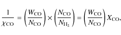
It is then possible to derive the atomic gas fraction,
if we assume that our absorption sample has similar properties. Writing
|
(1) |
taking the first term from our analysis of the results of Heiles & Troland (2003) and the second from the mean for the data shown in Fig. 1. The result is that
This estimate of the molecular gas fraction for our sample of
sightlines
falls in the middle of the range of current general estimates for
diffuse
gas as noted in the beginning of this Section, i.e. ![]() from
Copernicus corrected for sampling biases (Bohlin et al. 1978) and
from
Copernicus corrected for sampling biases (Bohlin et al. 1978) and
![]() from
a sample of lines of sight observed toward bright
stars in optical absorption lines observed in CH (Liszt
& Lucas 2002),
given that
from
a sample of lines of sight observed toward bright
stars in optical absorption lines observed in CH (Liszt
& Lucas 2002),
given that ![]() is nearly constant at
is nearly constant at ![]() (Sheffer
et al. 2008; Weselak et al. 2010).
(Sheffer
et al. 2008; Weselak et al. 2010).
3.4 Checking the molecular gas fraction via molecular chemistry
Shown in the middle panel is the integrated ![]() absorption. As noted in Sect. 2.3 the integrated optical depth
is
directly translatable into
absorption. As noted in Sect. 2.3 the integrated optical depth
is
directly translatable into ![]() column density given the near-absence of rotational excitation in the
relatively low density diffuse gas:
column density given the near-absence of rotational excitation in the
relatively low density diffuse gas: ![]() .
The relative abundance of
.
The relative abundance of ![]() is known to be
nearly constant at
is known to be
nearly constant at ![]() from its fixed ratio
with respect to OH in individual clouds (Liszt & Lucas 1996,2000)
and the
near-constancy of
from its fixed ratio
with respect to OH in individual clouds (Liszt & Lucas 1996,2000)
and the
near-constancy of ![]()
![]() (Weselak et al. 2010).
(Weselak et al. 2010).
Figure 1
shows that ![]() becomes readily detectable at
becomes readily detectable at ![]() mag,
which is just where
mag,
which is just where ![]() itself becomes abundant in the diffuse ISM
(Savage et al. 1977).
When detected,
itself becomes abundant in the diffuse ISM
(Savage et al. 1977).
When detected, ![]() shows a correlation with EB-V
(correlation coefficient 0.66 and power law slope 0.7 for the points
with
detected
shows a correlation with EB-V
(correlation coefficient 0.66 and power law slope 0.7 for the points
with
detected ![]() )
but the larger scatter in the middle panel, compared to
that at left, suggests that the molecular portion of the gas is
less well mixed than the absorbing
)
but the larger scatter in the middle panel, compared to
that at left, suggests that the molecular portion of the gas is
less well mixed than the absorbing ![]() .
.
If ![]() is assumed, a value for
is assumed, a value for ![]() could be derived from the data in
the middle panel of Fig. 1.
Conversely, if
could be derived from the data in
the middle panel of Fig. 1.
Conversely, if ![]() = 0.35 is assumed and
sample means are used, then
= 0.35 is assumed and
sample means are used, then ![]() and
and ![]() ,
consistent with the previously established value
(Liszt
& Lucas 1996,2000). Therefore
the decomposition of the ensemble of
lines of sight appears to yield consistent results between several
independent measures of both the atomic and molecular components.
,
consistent with the previously established value
(Liszt
& Lucas 1996,2000). Therefore
the decomposition of the ensemble of
lines of sight appears to yield consistent results between several
independent measures of both the atomic and molecular components.
3.5 The
ensemble-averaged CO luminosity and N
/W
conversion factor
Shown at the right in Fig. 1
is the integrated ![]() J=1-0 intensity
J=1-0 intensity
![]() plotted against EB-V.
CO emission is not reliably detected except
at
plotted against EB-V.
CO emission is not reliably detected except
at ![]() mag
(i.e.
mag
(i.e. ![]()
![]() 1 mag). In discussing this data, it is
important to note that values of
1 mag). In discussing this data, it is
important to note that values of ![]() have been measured in the diffuse
gas (Liszt &
Lucas 1998) and they are quite small compared to the column
of
free gas phase carbon expected at
have been measured in the diffuse
gas (Liszt &
Lucas 1998) and they are quite small compared to the column
of
free gas phase carbon expected at ![]() = 1 mag
(i.e.
= 1 mag
(i.e. ![]() ,
see Sofia et al. 2004).
Moreover, the lines of sight having the largest values of
,
see Sofia et al. 2004).
Moreover, the lines of sight having the largest values of ![]() are composed of several emission
components (see Appendix A for an example). The CO emission
along
these lines of sight orginates in diffuse gas where C+
is the dominant
form of carbon.
are composed of several emission
components (see Appendix A for an example). The CO emission
along
these lines of sight orginates in diffuse gas where C+
is the dominant
form of carbon.
If it is accepted that ![]() = 0.35, the bulk CO-
= 0.35, the bulk CO-
![]() conversion factor may be inferred immediately from the data shown in
Fig. 1.
The sample means are
conversion factor may be inferred immediately from the data shown in
Fig. 1.
The sample means are
![]() =
4.42
=
4.42
![]() and
and ![]() =
0.888 mag or
(
=
0.888 mag or
(
![]() ),
implying
),
implying ![]() =
1
=
1
![]() per
per
![]() .
Rather strikingly, there is
apparently no difference in the mean CO luminosity
per
.
Rather strikingly, there is
apparently no difference in the mean CO luminosity
per ![]() in
diffuse and fully molecular gas. For insight into the scatter
present in the ensemble of sightlines, the right-hand panel of
Fig. 1
shows a line corresponding to the ensemble mean conversion factor and
in
diffuse and fully molecular gas. For insight into the scatter
present in the ensemble of sightlines, the right-hand panel of
Fig. 1
shows a line corresponding to the ensemble mean conversion factor and ![]() .
The range in
.
The range in ![]() determined for the diffuse gas, roughly 0.25-0.45 or
determined for the diffuse gas, roughly 0.25-0.45 or ![]() ,
implies a 30% margin of
error for the method as a whole.
,
implies a 30% margin of
error for the method as a whole.
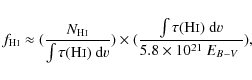
An alternative approach to this determination based on
molecular
chemistry, comparing ![]() with
with ![]() as
a surrogate for
as
a surrogate for ![]() and giving similar results, is discussed in Appendix C.
and giving similar results, is discussed in Appendix C.
![\begin{figure}
\par\includegraphics[height=7.3cm,clip]{14510f2.eps} \vspace*{-2.5mm}
\end{figure}](/articles/aa/full_html/2010/10/aa14510-10/img70.png)
|
Figure 2:
Integrated CO brightness plotted against 1/sin(|b|).
For comparison, a line is shown for the case of a plane-parallel
Gaussian layer with vertical dispersion |
| Open with DEXTER | |
4 The proportion of CO emission arising from diffuse gas
The similarity of the CO-
![]() conversion factors in diffuse and fully
molecular gas must have led to confusion whereby CO emission arising in
diffuse gas has been attributed to ``molecular clouds'', i.e. the
truism
noted in the Introduction. To quantify this phenomenon we derive the
mean
luminosity of diffuse molecular gas viewed perpendicular to the
galactic
plane
conversion factors in diffuse and fully
molecular gas must have led to confusion whereby CO emission arising in
diffuse gas has been attributed to ``molecular clouds'', i.e. the
truism
noted in the Introduction. To quantify this phenomenon we derive the
mean
luminosity of diffuse molecular gas viewed perpendicular to the
galactic
plane ![]() for a plane-parallel stratified gas layer
and we compare that to the equivalent luminosity perpendicular to the
galactic plane inferred from surveys of CO emission near the galactic
equator.
for a plane-parallel stratified gas layer
and we compare that to the equivalent luminosity perpendicular to the
galactic plane inferred from surveys of CO emission near the galactic
equator.
Shown in Fig. 2
is the distribution of ![]() with
with ![]() .
For
reference a line is shown corresponding to the canonical CO-
.
For
reference a line is shown corresponding to the canonical CO-
![]() conversion
factor and the combination
conversion
factor and the combination ![]() pc,
in the
simplistic case that the galactic gas layer can be described by a
single
Gaussian vertical component with dispersion
pc,
in the
simplistic case that the galactic gas layer can be described by a
single
Gaussian vertical component with dispersion ![]() .
For
convenience the diffuse gas is usually described by several components
having a range of vertical scale heights (Cox
2005) but the neutral gas
components of the nearby ISM are not well-described by simple
plane-parallel layers (see also Heiles
& Troland 2003) owing to local geometry
(the local bubble) combined with the scatter induced by the
comparatively
long mean free paths between kinematic components.
.
For
convenience the diffuse gas is usually described by several components
having a range of vertical scale heights (Cox
2005) but the neutral gas
components of the nearby ISM are not well-described by simple
plane-parallel layers (see also Heiles
& Troland 2003) owing to local geometry
(the local bubble) combined with the scatter induced by the
comparatively
long mean free paths between kinematic components.
We quote the ensemble average brightness ![]()
![]() and
number of equivalent half-thicknesses
and
number of equivalent half-thicknesses ![]() = 19.75,
implying a mean integrated brightness 0.235
= 19.75,
implying a mean integrated brightness 0.235
![]() per galactic
half width
per galactic
half width![]() . Looking down on the Milky
Way vertically from afar the integrated CO brightness of diffuse gas
would be twice this,
. Looking down on the Milky
Way vertically from afar the integrated CO brightness of diffuse gas
would be twice this, ![]() .
.
Galactic surveys of CO emission, on the other hand, calculate
a mean CO
brightness per kpc of 5
![]() /kpc
at z = 0 pc in the galactic disk
at a galactocentric distance
/kpc
at z = 0 pc in the galactic disk
at a galactocentric distance ![]() kpc.
Note that this value is scaled from the result of Burton & Gordon (1978)
which assumed
kpc.
Note that this value is scaled from the result of Burton & Gordon (1978)
which assumed ![]() kpc.
If the molecular gas layer sampled in these surveys is described by a
Gaussian vertical distribution having a dispersion
kpc.
If the molecular gas layer sampled in these surveys is described by a
Gaussian vertical distribution having a dispersion ![]() =
60 pc (Cox 2005)
and z-integral
=
60 pc (Cox 2005)
and z-integral ![]() kpc,
the galactic survey result translates into an integrated CO brightness
kpc,
the galactic survey result translates into an integrated CO brightness ![]() kpc
= 0.75
kpc
= 0.75
![]() when viewed vertically across the galactic disk
as described in Appendix D. This is only 50% higher than that
of the diffuse CO alone.
when viewed vertically across the galactic disk
as described in Appendix D. This is only 50% higher than that
of the diffuse CO alone.
The question then is whether the CO emission and ![]() attributable to diffuse gas exist in addition to that sampled in the CO
surveys near the galactic plane, or whether the galactic CO surveys
incorporate a significant proportion of diffuse CO emission. If the
former - if, for instance the diffuse CO like the diffuse ISM has a
larger scale height and is a distinguishable component of the local CO
emission - the local
attributable to diffuse gas exist in addition to that sampled in the CO
surveys near the galactic plane, or whether the galactic CO surveys
incorporate a significant proportion of diffuse CO emission. If the
former - if, for instance the diffuse CO like the diffuse ISM has a
larger scale height and is a distinguishable component of the local CO
emission - the local ![]() surface density could be higher than previously believed.
surface density could be higher than previously believed.
The total density of gas near the Sun is usually quoted as 1.2
H-nuclei
![]() from Spitzer (1978) and this
is often decomposed into ``molecular''
and ``diffuse'' components with roughly 50% attributed to each (for
instance see Cox 2005). The CO
emissivity measured in galactic plane
surveys (5
from Spitzer (1978) and this
is often decomposed into ``molecular''
and ``diffuse'' components with roughly 50% attributed to each (for
instance see Cox 2005). The CO
emissivity measured in galactic plane
surveys (5 ![]() /kpc)
conveniently converts to a local mean
/kpc)
conveniently converts to a local mean ![]() density of
about
density of
about ![]() ,
about half of Spitzer's total. However, recall
that the quoted total mean density is based on the statistics of
reddening
toward A-stars within a few hundred pc of the Sun (Münch
1952) which were
very unlikely to have sampled dark cloud lines of sight. GAIA
photometry should settle this matter, but the issue of the total
mean density of the ISM locally and relative proportions of atomic and
molecular material are not as clearly defined as is generally assumed.
,
about half of Spitzer's total. However, recall
that the quoted total mean density is based on the statistics of
reddening
toward A-stars within a few hundred pc of the Sun (Münch
1952) which were
very unlikely to have sampled dark cloud lines of sight. GAIA
photometry should settle this matter, but the issue of the total
mean density of the ISM locally and relative proportions of atomic and
molecular material are not as clearly defined as is generally assumed.
5
Rationale for a common CO-H
conversion
The very first discussions of the applicability of a common ![]() conversion
factor (Liszt
1982; Young
& Scoville 1982) noted that diffuse and dense gas
at 60-100 K, or dark dense gas at 12 K, all had
similar ratios
conversion
factor (Liszt
1982; Young
& Scoville 1982) noted that diffuse and dense gas
at 60-100 K, or dark dense gas at 12 K, all had
similar ratios ![]() /
/
![]() .
For instance
.
For instance ![]() ,
,
![]() toward
toward
![]() Oph (a
typical diffuse line of sight) and
Oph (a
typical diffuse line of sight) and ![]() ,
,
![]() toward
Ori A. By comparison, a dark cloud like L204, near
toward
Ori A. By comparison, a dark cloud like L204, near ![]() Oph, with
Oph, with ![]() = 5
mag has
= 5
mag has ![]() ,
,
![]() and
an integrated brightness
and
an integrated brightness ![]() (Tachihara et al. 2000)
or
(Tachihara et al. 2000)
or ![]() (K km s)-1.
Comparing the two gas phases sampled in CO near
(K km s)-1.
Comparing the two gas phases sampled in CO near ![]() Oph it is apparent that the higher CO column density in the dark cloud
is
more than compensated by the diminished brightness per CO
molecule. The result is a nearly constant ratio of
Oph it is apparent that the higher CO column density in the dark cloud
is
more than compensated by the diminished brightness per CO
molecule. The result is a nearly constant ratio of ![]() to
to ![]() across phases while the brightness per CO molecule
across phases while the brightness per CO molecule ![]() varies
widely.
varies
widely.
The physical basis for this behavior has become more apparent
recently with closer study of CO in diffuse gas (Pety et al. 2008; Liszt
et al. 2009).
To begin the discussion we rewrite the CO-
![]() conversion factor
conversion factor
![]() as
as
|
(2) |
separating the coupled and competing effects of cloud structure or radiative transfer
As noted by Goldreich
& Kwan (1974) in the original exposition of the LVG
model for
radiative transfer, ![]() /
/
![]() will
be much greater when the excitation of CO
is weak - when the kinetic temperature is much greater than the J=1-0
excitation temperature. Moreover when CO is excited somewhat above the
cosmic microwave background but well below the kinetic temperature, the
brightness of the CO J=1-0 line will be linearly
proportional to
will
be much greater when the excitation of CO
is weak - when the kinetic temperature is much greater than the J=1-0
excitation temperature. Moreover when CO is excited somewhat above the
cosmic microwave background but well below the kinetic temperature, the
brightness of the CO J=1-0 line will be linearly
proportional to ![]() even when the line is quite optically thick (again, see Goldreich & Kwan 1974).
As Michel Guelin pointedly reminded us, this occurs because weak
excitation means that
there is also little collisional de-excitation so that the gas merely
scatters emitted photons until they eventually escape. As Goldreich & Kwan (1974)
showed, this proportionality between brightness and column density
persists until the opacity is so very large that the transition
approaches
thermalization through radiative trapping.
even when the line is quite optically thick (again, see Goldreich & Kwan 1974).
As Michel Guelin pointedly reminded us, this occurs because weak
excitation means that
there is also little collisional de-excitation so that the gas merely
scatters emitted photons until they eventually escape. As Goldreich & Kwan (1974)
showed, this proportionality between brightness and column density
persists until the opacity is so very large that the transition
approaches
thermalization through radiative trapping.
The discussion of the previous paragraph also applies to other
molecules, but because CO has such a small dipole moment the
proportionality between CO brightness and column density is only weakly
dependent on ambient physical conditions: a nearly universal ratio ![]() can be
calculated for diffuse gas using recent excitation
cross-sections (Liszt 2007b).
This is in excellent agreement with measured
values of
can be
calculated for diffuse gas using recent excitation
cross-sections (Liszt 2007b).
This is in excellent agreement with measured
values of ![]() and CO J= 1-0 excitation temperatures in the
diffuse gas
seen toward stars in uv absorption (Sheffer et al. 2008; Burgh
et al. 2007; Sonnentrucker et al. 2007)
or
at mm-wavelengths in absorption against distant quasars
(Liszt & Lucas
1998). For the observed value
and CO J= 1-0 excitation temperatures in the
diffuse gas
seen toward stars in uv absorption (Sheffer et al. 2008; Burgh
et al. 2007; Sonnentrucker et al. 2007)
or
at mm-wavelengths in absorption against distant quasars
(Liszt & Lucas
1998). For the observed value ![]() (Burgh et al. 2007) the
(Burgh et al. 2007) the ![]() /
/
![]() conversion
ratio in diffuse clouds is
conversion
ratio in diffuse clouds is ![]() /
/
![]()
![]() .
.
Finally, note that even if the ratio ![]() /
/
![]() is
not constant between gas phases, it is still the case that
is
not constant between gas phases, it is still the case that ![]() separately in either the dense or diffuse gas. For the diffuse gas the
proportionality is based in the microphysics of CO radiative transfer a
la Goldreich & Kwan (1974).
For the dark cloud case, note that there is a fixed ratio of
separately in either the dense or diffuse gas. For the diffuse gas the
proportionality is based in the microphysics of CO radiative transfer a
la Goldreich & Kwan (1974).
For the dark cloud case, note that there is a fixed ratio of ![]() /
/
![]() when
the gas-phase carbon is in CO and the hydrogen is in
when
the gas-phase carbon is in CO and the hydrogen is in ![]() so that a
so that a ![]() -
-
![]() conversion
is fully equivalent to a
conversion
is fully equivalent to a ![]() -
-
![]() conversion.
conversion.
6 Discriminating between emission from diffuse and dense gas
There are ways in which mm-wave molecular emission differs between
dense
and diffuse gas, even if not in ![]() .
Emission from molecules like CS,
HCN and
.
Emission from molecules like CS,
HCN and ![]() having higher dipole moments is generally thought to single
out denser gas than does CO, especially in extreme environments
(Wu et al. 2005).
Note, however, that surveys of the Milky Way
galactic plane find widely-distributed emission in
having higher dipole moments is generally thought to single
out denser gas than does CO, especially in extreme environments
(Wu et al. 2005).
Note, however, that surveys of the Milky Way
galactic plane find widely-distributed emission in ![]() ,
CS, HCN, etc. with intensity ratios of 1-2% relative to
,
CS, HCN, etc. with intensity ratios of 1-2% relative to ![]() from essentially all features detected in CO (Helfer & Blitz 1997; Liszt 1995).
from essentially all features detected in CO (Helfer & Blitz 1997; Liszt 1995).
Relatively little is known of the emission from mm-wave
species in diffuse
gas beyond that from CO. Most common is emission from ![]() because it is
chemically ubiquitous and somewhat more easily excited owing to
its positive charge and high dipole moment. Although
because it is
chemically ubiquitous and somewhat more easily excited owing to
its positive charge and high dipole moment. Although ![]() emission is
weak in the example shown here in Appendix A it appears at
levels
emission is
weak in the example shown here in Appendix A it appears at
levels
![]() 1% of
1% of ![]() in portions of the diffuse cloud around
in portions of the diffuse cloud around ![]() Oph or in the Polaris flare (Liszt 1997; Liszt & Lucas 1994; Falgarone
et al. 2006). Therefore
Oph or in the Polaris flare (Liszt 1997; Liszt & Lucas 1994; Falgarone
et al. 2006). Therefore ![]() emission is probably not
a good discriminator but CS and HCN appear with high abundance only
when
emission is probably not
a good discriminator but CS and HCN appear with high abundance only
when
![]()
![]() or
or
![]() and should be
much more weakly excited in low density gas. In any case, searching for
emission that is 100 times weaker than
and should be
much more weakly excited in low density gas. In any case, searching for
emission that is 100 times weaker than ![]() may not be an effective use of
observing time and only in very dense, warmer gas like that found in
massive, OB star-forming regions like Ori A are the higher dipole
moment
molecules substantially brighter than 1-2% relative to
may not be an effective use of
observing time and only in very dense, warmer gas like that found in
massive, OB star-forming regions like Ori A are the higher dipole
moment
molecules substantially brighter than 1-2% relative to ![]() .
.
A more effective method of discriminating between CO emission
from diffuse
and dark or dense gas is afforded by ![]() .
Although the abundance of
.
Although the abundance of
![]() is enhanced by fractionation (see the example in Appendix A)
lowering the observed
is enhanced by fractionation (see the example in Appendix A)
lowering the observed ![]() /
/
![]() brightness
temperature ratios
(Liszt 2007b;
Liszt
& Lucas 1998; Goldsmith et al. 2008),
those ratios are still noticeably higher
in diffuse gas. Typically they are
brightness
temperature ratios
(Liszt 2007b;
Liszt
& Lucas 1998; Goldsmith et al. 2008),
those ratios are still noticeably higher
in diffuse gas. Typically they are ![]() 10-15 instead of
10-15 instead of ![]() 3-5 as
seen in dark clouds or in surveys of the inner-Galaxy gas in the
galactic plane
(Burton & Gordon 1978).
Recall that the mean
3-5 as
seen in dark clouds or in surveys of the inner-Galaxy gas in the
galactic plane
(Burton & Gordon 1978).
Recall that the mean ![]() /
/
![]() brightness
ratio
nearly doubles across the galactic disk (Liszt
et al. 1981), which was
another, earlier indication that molecular gas near the Solar Circle
has a
high proportion of diffuse material.
brightness
ratio
nearly doubles across the galactic disk (Liszt
et al. 1981), which was
another, earlier indication that molecular gas near the Solar Circle
has a
high proportion of diffuse material.
To summarize, we suggest that the most efficient way to
ascertain the
origin of CO emission is to compare ![]() and
and ![]() brightnesses because
emission from
brightnesses because
emission from ![]() is much stronger than emission from
is much stronger than emission from ![]() ,
CS, HCN
etc., and because there is actually less ambiguity in the brightness
ratios
relative to
,
CS, HCN
etc., and because there is actually less ambiguity in the brightness
ratios
relative to ![]() .
.
7 Summary
In Sects. 2 and 3 we described and
considered a sample of lines of sight
studied in ![]() and molecular absorption and known to be comprised
of diffuse gas. Their molecular component shows features whose CO,
and molecular absorption and known to be comprised
of diffuse gas. Their molecular component shows features whose CO,
![]() and other molecular column densities are small compared to those of
dark clouds (in the case of CO, at least 30 times smaller). There is
often quite substantial fractionation of
and other molecular column densities are small compared to those of
dark clouds (in the case of CO, at least 30 times smaller). There is
often quite substantial fractionation of ![]() (indicating that the dominant form of carbon is C+)
and the rotational excitation of CO is sub-thermal
with implied cloud temperatures typical of those determined directly
for diffuse
(indicating that the dominant form of carbon is C+)
and the rotational excitation of CO is sub-thermal
with implied cloud temperatures typical of those determined directly
for diffuse ![]() in optical/uv surveys, i.e. 30 K or more.
in optical/uv surveys, i.e. 30 K or more.
Using an externally-determined value for the ratio of total ![]() column
density to integrated
column
density to integrated ![]() absorption and the standard equivalence between
reddening and
absorption and the standard equivalence between
reddening and ![]() we derived the molecular gas fraction for this sample
to be
we derived the molecular gas fraction for this sample
to be ![]() =
0.35, in the middle of the range of other estimates for the
diffuse ISM as a whole based on optical (mainly CH) and uv (
=
0.35, in the middle of the range of other estimates for the
diffuse ISM as a whole based on optical (mainly CH) and uv (
![]() and
and ![]() )
absorption studies.
)
absorption studies.
We showed that this estimate for ![]() implies the same value
implies the same value ![]() that was previously determined from comparisons of OH and
that was previously determined from comparisons of OH and
![]() column densities in individual clouds. We then compared measured CO
brightnesses with the inferred molecular gas column densities to
derive the ensemble mean
column densities in individual clouds. We then compared measured CO
brightnesses with the inferred molecular gas column densities to
derive the ensemble mean ![]() conversion factor. Surprisingly, We
found this mean to be just equal to the locally-accepted value
conversion factor. Surprisingly, We
found this mean to be just equal to the locally-accepted value ![]() /(
/(
![]() )
for ``molecular'' gas believed to reside in dense
dark fully-molecular clouds near the galactic equator.
)
for ``molecular'' gas believed to reside in dense
dark fully-molecular clouds near the galactic equator.
Such exact agreement is probably something of an accident of
sampling, but
the fact that diffuse and dark gas would have very similar ![]() conversion
factors, which had been inferred empirically long ago, now has a
firmer physical basis. In Sect. 5 we explained it as the
result of the
brightening of CO J=1-0 emission per CO molecule
that was theoretically
predicted for warmer more diffuse gas by Goldreich
& Kwan (1974), which
compensates for the lower relative abundance
conversion
factors, which had been inferred empirically long ago, now has a
firmer physical basis. In Sect. 5 we explained it as the
result of the
brightening of CO J=1-0 emission per CO molecule
that was theoretically
predicted for warmer more diffuse gas by Goldreich
& Kwan (1974), which
compensates for the lower relative abundance ![]() there. The mean
CO abundance observed in optical absorption in diffuse clouds
there. The mean
CO abundance observed in optical absorption in diffuse clouds ![]() ,
combined with the observed and expected
brightness per CO molecule,
,
combined with the observed and expected
brightness per CO molecule, ![]() /
/
![]() =
1
=
1 ![]() /
/
![]() ,
can be be combined to form an CO-
,
can be be combined to form an CO-
![]() conversion factor of
conversion factor of ![]() /
/
![]()
![]() .
.
In Sect. 4 we derived the expected brightness of
diffuse gas viewed
perpendicular to the galactic plane from afar, 0.47
![]() ,
and compared that
to the value expected from surveys of CO emission in the galactic
plane,
combined with a narrow (60 pc dispersion) Gaussian vertical
distribution;
that is 0.75
,
and compared that
to the value expected from surveys of CO emission in the galactic
plane,
combined with a narrow (60 pc dispersion) Gaussian vertical
distribution;
that is 0.75
![]() .
This suggests that there has been confusion in the
general attribution of CO emission to ``molecular clouds'' when in fact
much of it arises in the diffuse ISM. This view is consistent with the
motivations discussed in the Introduction, whereby CO emission is
increasingly being found along lines of sight lacking high extinction
and
whereby CO emission seen along dark lines of sight is found (through
molecular absorption studies and in other ways) to originate in
components having the relatively small molecular number and column
densities typical of diffuse gas. An example of such a line of sight is
given in Appendix A here.
.
This suggests that there has been confusion in the
general attribution of CO emission to ``molecular clouds'' when in fact
much of it arises in the diffuse ISM. This view is consistent with the
motivations discussed in the Introduction, whereby CO emission is
increasingly being found along lines of sight lacking high extinction
and
whereby CO emission seen along dark lines of sight is found (through
molecular absorption studies and in other ways) to originate in
components having the relatively small molecular number and column
densities typical of diffuse gas. An example of such a line of sight is
given in Appendix A here.
We briefly discussed in Sect. 4 the decomposition of
the total mean density
of neutral gas in the nearby ISM, 1.2 H
![]() (Spitzer 1978), into its
atomic and molecular constituents. We noted that although the balance
is
generally believed to be roughly 50-50 (Cox
2005), some emission might
shift to the diffuse side of the balance sheet if CO emission is
reinterpreted. Moreover, we pointed out that the molecular contribution
to the true local mean density from large-scale galactic CO surveys in
the galactic plane should be questioned more generally because it is
unclear to what extent Spitzer's estimate, based on the earlier optical
work of Münch, incorporates the contribution of optically-opaque gas.
(Spitzer 1978), into its
atomic and molecular constituents. We noted that although the balance
is
generally believed to be roughly 50-50 (Cox
2005), some emission might
shift to the diffuse side of the balance sheet if CO emission is
reinterpreted. Moreover, we pointed out that the molecular contribution
to the true local mean density from large-scale galactic CO surveys in
the galactic plane should be questioned more generally because it is
unclear to what extent Spitzer's estimate, based on the earlier optical
work of Münch, incorporates the contribution of optically-opaque gas.
Although the ability to discriminate between the separate
contributions to
![]() from diffuse and darker, denser gas is limited when only
from diffuse and darker, denser gas is limited when only ![]() is considered,
it should be possible to infer the nature of the host gas using other
emission diagnostics (see Sect. 6). The most efficient of
these is
probably the brightness of
is considered,
it should be possible to infer the nature of the host gas using other
emission diagnostics (see Sect. 6). The most efficient of
these is
probably the brightness of ![]() ,
which, although enhanced by
fractionation, is still substantially weaker, relative to
,
which, although enhanced by
fractionation, is still substantially weaker, relative to ![]() ,
in diffuse
gas. Searching for emission from species having higher dipole moments
such
as CS J=2-1 and HCN (and probably not
,
in diffuse
gas. Searching for emission from species having higher dipole moments
such
as CS J=2-1 and HCN (and probably not ![]() because it is chemically so
ubiquitous and more easily excited) are alternatives that might require
somewhat longer integration times.
because it is chemically so
ubiquitous and more easily excited) are alternatives that might require
somewhat longer integration times.
8 Discussion: Interpreting a sky occupied by CO emission from diffuse gas
The usual interpretation of CO sky maps, galactic surveys,
etc, is that CO
emission mostly traces dark and or ``giant'' molecular clouds (GMC)
composed
of dense cold gas occupying a very small fraction of the interstellar
volume at high thermal pressure within an ISM that may confine them via
its
ram or turbulent pressure if they are not gravitationally bound. The
balance between GMC and diffuse atomic material may be controlled by
quasi-equilibrium between local dynamics and the overlying weight of
the
gas layer but the molecular material inferred from CO emission is
generally
believed to be that which is most nearly on the verge of forming stars,
for
instance through the Schmidt-Kenicutt power-law relation between star
formation rate and gas surface density![]() (Bigiel
et al. 2008; Leroy et al. 2008).
(Bigiel
et al. 2008; Leroy et al. 2008).
By contrast, CO emission from diffuse molecular gas originates
within a
warmer, lower-pressure medium that occupies a much larger fraction of
the
volume and contributes more substantially to mid-IR dust or PAH
emission
but only has the requisite density and chemistry to produce CO
molecules
and CO emission (since ![]() )
over a very limited portion of
that volume. In this case a map of CO emission is a map of CO abundance
and CO chemistry first, and only secondarily a map of the mass even if
the
mean CO-
)
over a very limited portion of
that volume. In this case a map of CO emission is a map of CO abundance
and CO chemistry first, and only secondarily a map of the mass even if
the
mean CO-
![]() conversion ratio is (as we have shown) ``standard''. Moreover,
although CO emission traces the molecular column density
conversion ratio is (as we have shown) ``standard''. Moreover,
although CO emission traces the molecular column density ![]() quite
decently where
quite
decently where ![]() is at detectable levels, it arises in regions that are
not gravitationally bound or about to form stars. The CO sky is
mostly an image of the CO chemistry.
is at detectable levels, it arises in regions that are
not gravitationally bound or about to form stars. The CO sky is
mostly an image of the CO chemistry.
The National Radio Astronomy Observatory is operated by Associated Universites, Inc. under a cooperative agreement with the US National Science Foundation. The Kitt Peak 12-m millimetre wave telescope is operated by the Arizona Radio Observatory (ARO), Steward Observatory, University of Arizona. IRAM is operated by CNRS (France), the MPG (Germany) and the IGN (Spain). This work has been partially funded by the grant ANR-09-BLAN-0231-01 from the French Agence Nationale de la Recherche as part of the SCHISM project. We thank Bob Garwood for providing the H I profiles of Dickey et al. (1983) in digital form.
Appendix A: NRAO150: an example of a dark line of sight comprised of diffuse gas
![\begin{figure}
\par\includegraphics[height=14cm,clip]{14510f3.eps}\vspace*{-3mm}
\end{figure}](/articles/aa/full_html/2010/10/aa14510-10/img112.png)
|
Figure A.1:
Line profiles toward and near B0355+508 = NRAO150. Bottom:
absorption line profiles of H I, |
| Open with DEXTER | |
The estimated total extinction along this comparatively low-latitude
line
of sight at l=150.4![]() ,
b=-1.6
,
b=-1.6![]() (see Table E.2) is EB-V =
1.5 mag
or
(see Table E.2) is EB-V =
1.5 mag
or ![]()
![]() mag
but it would be quite opaque even if only the atomic
gas were present. A lower limit on
mag
but it would be quite opaque even if only the atomic
gas were present. A lower limit on ![]() from the integrated 21 cm
emission of the nearest profile in the Leiden-Dwingeloo Survey
(Hartmann & Burton 1997)
in the optically thin limit is
from the integrated 21 cm
emission of the nearest profile in the Leiden-Dwingeloo Survey
(Hartmann & Burton 1997)
in the optically thin limit is ![]() ,
implying EB-V
,
implying EB-V ![]() mag.
The H I column
density derived by taking the ratio of
mag.
The H I column
density derived by taking the ratio of ![]() to
to ![]() absorption
as discussed in Sect. 3 here is, understandably, slightly
larger,
absorption
as discussed in Sect. 3 here is, understandably, slightly
larger,
![]() .
.
We show in Fig. A.1
various absorption and emission profiles along
and around the line of sight to NRAO150 aka B0355+508. We have
published various analyses of this line of sight in the references
noted
below, and most recently we synthesized the CO emission in a 90
![]() region around NRAO150 at 6
region around NRAO150 at 6
![]() resolution (Pety et al. 2008).
resolution (Pety et al. 2008).
![]() absorption
and emission extend well outside the narrow
kinematic interval shown here. The weak
absorption
and emission extend well outside the narrow
kinematic interval shown here. The weak ![]() absorption at -35 km s-1 is
real, as is the broad wing extending up to -25 km s-1.
absorption at -35 km s-1 is
real, as is the broad wing extending up to -25 km s-1.
CO emission is fairly strong in this direction, ![]() = 17 K km s-1,
nominally implying 2
= 17 K km s-1,
nominally implying 2
![]()
![]() ,
comparable to
,
comparable to
![]() ,
but molecular absorption spectra of
,
but molecular absorption spectra of ![]() and CO are much
richer than the CO emission. The
and CO are much
richer than the CO emission. The ![]() absorption spectrum
(Liszt
& Lucas 2000; Lucas & Liszt 1996)
shows five prominent components each having
absorption spectrum
(Liszt
& Lucas 2000; Lucas & Liszt 1996)
shows five prominent components each having
![]()
![]() (Lucas & Liszt
1996) or 2
(Lucas & Liszt
1996) or 2
![]()
![]() implying EB-V =
0.15 mag per component
associated with
implying EB-V =
0.15 mag per component
associated with ![]() if
if ![]() as discussed in Sect. 3. The
as discussed in Sect. 3. The ![]() ,
,
![]() and
OH column densities of these components are each nearly equal to what
is seen locally along the line of sight to
and
OH column densities of these components are each nearly equal to what
is seen locally along the line of sight to ![]() Oph at
Oph at ![]() = 1 mag (Liszt
1997; Morton
1975; Van
Dishoeck & Black 1986).
= 1 mag (Liszt
1997; Morton
1975; Van
Dishoeck & Black 1986).
Further evidence of the diffuse nature of the gas is given by
the
fractionation of ![]() in CO;
in CO; ![]() ,
,
![]() and
and ![]() in the components at -17, -11 and -4 km s-1,
respectively and
in the components at -17, -11 and -4 km s-1,
respectively and ![]() ,
>54 and >25 at
the
,
>54 and >25 at
the ![]() level in these components (Liszt
& Lucas 1998).
level in these components (Liszt
& Lucas 1998).
In emission, the ![]() /
/
![]() brightness
ratios are 12 and 30 for the two
strong kinematic components, reflecting both the fractionation and the
fact
that
brightness
ratios are 12 and 30 for the two
strong kinematic components, reflecting both the fractionation and the
fact
that ![]() in the diffuse gas regime as discussed in the text here.
in the diffuse gas regime as discussed in the text here.
![]() emission
is weak in Fig. A.1.
The profile shown
(from Lucas &
Liszt 1996) is an average of positions around the continuum
source to avoid contamination from absorption. The low levels of
emission
is weak in Fig. A.1.
The profile shown
(from Lucas &
Liszt 1996) is an average of positions around the continuum
source to avoid contamination from absorption. The low levels of ![]() emission seen toward our sample of background continuum sources can be
understood as arising from relatively low density gas (
emission seen toward our sample of background continuum sources can be
understood as arising from relatively low density gas (
![]() )
when the electron fraction is as high as expected for diffuse gas,
i.e.
)
when the electron fraction is as high as expected for diffuse gas,
i.e. ![]() (Lucas
& Liszt 1994,1996).
(Lucas
& Liszt 1994,1996).
Appendix B: The ratio of total to absorbing H I
![\begin{figure}
\par\includegraphics[height=6.5cm,clip]{14510f4.eps}
\end{figure}](/articles/aa/full_html/2010/10/aa14510-10/img129.png)
|
Figure B.1:
Total hydrogen column density vs. integrated |
| Open with DEXTER | |
Shown in Fig. B.1
is a plot of the data from the tables of Heiles
& Troland (2003)
that were used in Sect. 3 to convert the ![]() measurements in Fig. 1
to
a total quantity of
measurements in Fig. 1
to
a total quantity of ![]() .
The plot shows a regression line (power-law
slope 0.84) fit to data points with EB-V >
0.09 mag (the range occupied
by the
.
The plot shows a regression line (power-law
slope 0.84) fit to data points with EB-V >
0.09 mag (the range occupied
by the ![]() detections in Fig. 1) to point out a
slight upturn at
low
detections in Fig. 1) to point out a
slight upturn at
low ![]() .
The sample means are largely unaffected by setting various
sample selection criteria.
.
The sample means are largely unaffected by setting various
sample selection criteria.
Appendix
C: A chemistry-based determination of N
/W
![\begin{figure}
\par\includegraphics[height=7cm,clip]{14510f5.eps}
\end{figure}](/articles/aa/full_html/2010/10/aa14510-10/img130.png)
|
Figure C.1:
Integrated CO J=1-0 brightness plotted
against the integrated |
| Open with DEXTER | |
It is also possible to determine ![]() /
/
![]() without
the H I measure
or formally estimating
without
the H I measure
or formally estimating ![]() ,
although we preferred not to do this
in the main discussion. In Fig. C.1 we show the
variation of
,
although we preferred not to do this
in the main discussion. In Fig. C.1 we show the
variation of ![]() with
with ![]() .
CO appears reliably at detectable levels
.
CO appears reliably at detectable levels ![]() ,
,
![]() when
when
![]() or
or ![]() .
If
.
If ![]() the
ensemble mean values
the
ensemble mean values ![]() ,
,
![]() imply
imply
![]() per
per ![]() ,
just 30%
above that derived in Sect. 3.5.
,
just 30%
above that derived in Sect. 3.5.
The near linearity of the ![]() -
-
![]() relationship
in Fig. C.1
results from bulk averaging over whole lines of sight: given the same
general mix of conditions, an ensemble of richer and poorer or shorter
and longer sightlines will show proportionalities between almost any
two quantities in this way. As shown in Fig. A.1 there is no such
proportionality on a per-component basis. In detail, and with much
scatter, the overall chemical variation is approximately
relationship
in Fig. C.1
results from bulk averaging over whole lines of sight: given the same
general mix of conditions, an ensemble of richer and poorer or shorter
and longer sightlines will show proportionalities between almost any
two quantities in this way. As shown in Fig. A.1 there is no such
proportionality on a per-component basis. In detail, and with much
scatter, the overall chemical variation is approximately ![]() (Sheffer
et al. 2008; Liszt 2007b).
(Sheffer
et al. 2008; Liszt 2007b).
Appendix D: Calculating the CO brightness from galactic survey results
The statistics of observing the clumpy galactic molecular cloud
distribution are Poisson (Gordon & Burton 1976; Burton &
Gordon 1978) so the integrated CO brightness ![]() (r)
accumulated when traversing a path of length r in the galactic
plane is
(r)
accumulated when traversing a path of length r in the galactic
plane is
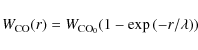
|
(3) |
where
The brightness of the CO cloud ensemble viewed vertically
through
the galactic disk is then just ![]() ,
where
,
where ![]() is
the equivalent thickness of the disk. For a Gaussian
vertical distribution with dispersion
is
the equivalent thickness of the disk. For a Gaussian
vertical distribution with dispersion ![]() ,
,
![]() .
.
References
- Bigiel, F., Leroy, A., Walter, F., et al. 2008, AJ., 136, 2846 [NASA ADS] [CrossRef] [Google Scholar]
- Bohlin, R. C., Savage, B. D., & Drake, J. F. 1978, ApJ, 224, 132 [NASA ADS] [CrossRef] [Google Scholar]
- Bothwell, M. S., Kennicutt, R. C., & Lee, J. C. 2009, MNRAS, 400, 154 [NASA ADS] [CrossRef] [Google Scholar]
- Burgh, E. B., France, K., & McCandliss, S. R. 2007, ApJ, 658, 446 [NASA ADS] [CrossRef] [Google Scholar]
- Burton, W. B., & Gordon, M. A. 1978, A&A, 63, 7 [NASA ADS] [Google Scholar]
- Cox, D. P. 2005, ARA&A, 43, 337 [NASA ADS] [CrossRef] [EDP Sciences] [MathSciNet] [Google Scholar]
- Dickey, J. M., Kulkarni, S. R., Heiles, C. E., & Van Gorkom, J. H. 1983, ApJSS, 53, 591 [CrossRef] [Google Scholar]
- Draine, B. T., Dale, D. A., Bendo, G., et al. 2007, ApJ, 663, 866 [NASA ADS] [CrossRef] [Google Scholar]
- Falgarone, E., Pineau Des Forêts, G., Hily-Blant, P., & Schilke, P. 2006, A&A, 452, 511 [NASA ADS] [CrossRef] [EDP Sciences] [Google Scholar]
- Garwood, R. W., & Dickey, J. M. 1989, ApJ, 338, 841 [NASA ADS] [CrossRef] [Google Scholar]
- Goldreich, P., & Kwan, J. 1974, ApJ, 189, 441 [NASA ADS] [CrossRef] [Google Scholar]
- Goldsmith, P. F., Heyer, M., Narayanan, G., et al. 2008, ApJ, 680, 428 [NASA ADS] [CrossRef] [Google Scholar]
- Gordon, M. A., & Burton, W. B. 1976, ApJ, 208, 346 [NASA ADS] [CrossRef] [Google Scholar]
- Hartmann, D., & Burton, W. B. 1997, Atlas of galactic neutral hydrogen (Cambridge; New York: Cambridge University Press) [Google Scholar]
- Heiles, C., & Troland, T. H. 2003, ApJ, 586, 1067 [NASA ADS] [CrossRef] [Google Scholar]
- Helfer, T. T., & Blitz, L. 1997, ApJ, 478, 233 [NASA ADS] [CrossRef] [Google Scholar]
- Leroy, A. K., Walter, F., Brinks, E., et al. 2008, AJ, 136, 2782 [NASA ADS] [CrossRef] [Google Scholar]
- Liszt, H. 1997a, A&ASS, 124, 183 [NASA ADS] [CrossRef] [EDP Sciences] [Google Scholar]
- Liszt, H. S. 1982, ApJ, 262, 198 [NASA ADS] [CrossRef] [Google Scholar]
- Liszt, H. S. 1995, ApJ, 442, 163 [NASA ADS] [CrossRef] [Google Scholar]
- Liszt, H. S. 1997, A&A, 322, 962 [NASA ADS] [Google Scholar]
- Liszt, H. S. 2007a, A&A, 476, 291 [NASA ADS] [CrossRef] [EDP Sciences] [Google Scholar]
- Liszt, H. S. 2007b, A&A, 461, 205 [NASA ADS] [CrossRef] [EDP Sciences] [Google Scholar]
- Liszt, H., & Lucas, R. 2002, A&A, 391, 693 [NASA ADS] [CrossRef] [EDP Sciences] [Google Scholar]
- Liszt, H. S., & Lucas, R. 1994, ApJ, 431, L131 [NASA ADS] [CrossRef] [Google Scholar]
- Liszt, H. S., & Lucas, R. 1996, A&A, 314, 917 [NASA ADS] [Google Scholar]
- Liszt, H. S., & Lucas, R. 1998, A&A, 339, 561 [NASA ADS] [Google Scholar]
- Liszt, H. S., & Lucas, R. 2000, A&A, 355, 333 [NASA ADS] [Google Scholar]
- Liszt, H. S., Burton, W. B., & Bania, T. M. 1981, ApJ, 246, 74 [NASA ADS] [CrossRef] [Google Scholar]
- Liszt, H. S., Pety, J., & Tachihara, K. 2009, A&A, 499, 503 [NASA ADS] [CrossRef] [EDP Sciences] [Google Scholar]
- Lucas, R., & Liszt, H. S. 1994, A&A, 282, L5 [Google Scholar]
- Lucas, R., & Liszt, H. S. 1996, A&A, 307, 237 [NASA ADS] [Google Scholar]
- McCall, B. J., Hinkle, K. H., Geballe, T. R., et al. 2002, ApJ, 567, 391 [NASA ADS] [CrossRef] [Google Scholar]
- Morton, D. C. 1975, ApJ, 197, 85 [NASA ADS] [CrossRef] [Google Scholar]
- Münch, I. G. 1952, ApJ, 116, 575 [Google Scholar]
- Pety, J., Lucas, R., & Liszt, H. S. 2008, A&A, 489, 217 [NASA ADS] [CrossRef] [EDP Sciences] [Google Scholar]
- Rachford, B. L., Snow, T. P., Destree, J. D., et al. 2009, ApJSS, 180, 125 [NASA ADS] [CrossRef] [Google Scholar]
- Savage, B. D., Drake, J. F., Budich, W., & Bohlin, R. C. 1977, ApJ, 216, 291 [NASA ADS] [CrossRef] [Google Scholar]
- Schlegel, D. J., Finkbeiner, D. P., & Davis, M. 1998, ApJ, 500, 525 [NASA ADS] [CrossRef] [Google Scholar]
- Sheffer, Y., Rogers, M., Federman, S. R., et al. 2008, ApJ, 687, 1075 [NASA ADS] [CrossRef] [Google Scholar]
- Sheffer, Y., Rogers, M., Federman, S. R., Lambert, D. L., & Gredel, R. 2007, ApJ, 667, 1002 [NASA ADS] [CrossRef] [Google Scholar]
- Sofia, U. J., Lauroesch, J. T., Meyer, D. M., & Cartledge, S. I. B. 2004, ApJ, 605, 272 [NASA ADS] [CrossRef] [Google Scholar]
- Sonnentrucker, P., Welty, D. E., Thorburn, J. A., & York, D. G. 2007, ApJSS, 168, 58 [NASA ADS] [CrossRef] [Google Scholar]
- Spitzer, L. 1978, Physical processes in the interstellar medium (New York: Wiley-Interscience) [Google Scholar]
- Tachihara, K., Abe, R., Onishi, T., Mizuno, A., & Fukui, Y. 2000, Publ. Astron. Soc. Jpn., 52, 1147 [Google Scholar]
- Van Dishoeck, E. F., & Black, J. H. 1986, ApJSS, 62, 109 [NASA ADS] [CrossRef] [Google Scholar]
- Watson, W. D., Anicich, V. G., & Huntress, W. T., J. 1976, ApJ, 205, L165 [NASA ADS] [CrossRef] [Google Scholar]
- Weselak, T., Galazutdinov, G. A., Beletsky, Y., & Kre▯owski, J. 2010, Mon. Not. R. Astron. Soc., 402, 1991 [Google Scholar]
- Wu, J., Evans, II, N. J., Gao, Y., et al. 2005, ApJ, 635, L173 [NASA ADS] [CrossRef] [Google Scholar]
- Young, J. S., & Scoville, N. 1982, ApJ, 258, 467 [NASA ADS] [CrossRef] [Google Scholar]
Online Material
Appendix E: Data
The data shown in Fig. 1 are tabulated in Tables E.1 and E.2. The sources of these data are discussed in Sect. 2.Table E.1: Data used in this work.
Table E.2: Data used in this work (continued).
Footnotes
- ... gas?
- Appendix E is only available in electronic form at http://www.aanda.org
- ... width
- The actual ensemble averaged value of
 is substantially larger
 .
.
- ... density
- It is also recognized that more precise tracers of the high-density star-forming material may be needed in extreme environments such as ULIRG (Wu et al. 2005).
All Tables
Table E.1: Data used in this work.
Table E.2: Data used in this work (continued).
All Figures
|
|
Figure 1:
Atomic and molecular absorption and emission vs. total reddening.
Left: Integrated VLA |
| Open with DEXTER | |
| In the text | |
|
|
Figure 2:
Integrated CO brightness plotted against 1/sin(|b|).
For comparison, a line is shown for the case of a plane-parallel
Gaussian layer with vertical dispersion |
| Open with DEXTER | |
| In the text | |
|
|
Figure A.1:
Line profiles toward and near B0355+508 = NRAO150. Bottom:
absorption line profiles of H I, |
| Open with DEXTER | |
| In the text | |
|
|
Figure B.1:
Total hydrogen column density vs. integrated |
| Open with DEXTER | |
| In the text | |
|
|
Figure C.1:
Integrated CO J=1-0 brightness plotted
against the integrated |
| Open with DEXTER | |
| In the text | |
Copyright ESO 2010
Current usage metrics show cumulative count of Article Views (full-text article views including HTML views, PDF and ePub downloads, according to the available data) and Abstracts Views on Vision4Press platform.
Data correspond to usage on the plateform after 2015. The current usage metrics is available 48-96 hours after online publication and is updated daily on week days.
Initial download of the metrics may take a while.