| Issue |
A&A
Volume 518, July-August 2010
Herschel: the first science highlights
|
|
|---|---|---|
| Article Number | A3 | |
| Number of page(s) | 4 | |
| Section | The Sun | |
| DOI | https://doi.org/10.1051/0004-6361/201014374 | |
| Published online | 18 August 2010 | |
Milne-Eddington inversion of the Fe I line pair at 630 nm
(Research Note)
D. Orozco Suárez1 - L. R. Bellot Rubio2 - J. C. del Toro Iniesta2
1 - National Astronomical Observatory of Japan, 2-21-1 Osawa,
Mitaka, Tokyo 181-8588, Japan
2 - Instituto de Astrofísica de Andalucía (CSIC), Apdo. Correos 3004, 18080 Granada, Spain
Received 8 March 2010 / Accepted 26 May 2010
Abstract
Context. The iron lines at 630.15 and 630.25 nm are
often used to determine the physical conditions of the solar
photosphere. A common approach is to invert them simultaneously under
the Milne-Eddington approximation. The same thermodynamic parameters
are employed for the two lines, except for their opacities, which are
assumed to have a constant ratio.
Aims. We aim at investigating the validity of this assumption, since the two lines are not exactly the same.
Methods. We use magnetohydrodynamic simulations of the quiet Sun
to examine the behavior of the ME thermodynamic parameters and their
influence on the retrieval of vector magnetic fields and flow
velocities.
Results. Our analysis shows that the two lines can be coupled
and inverted simultaneously using the same thermodynamic parameters and
a constant opacity ratio. The inversion of two lines is significantly
more accurate than single-line inversions because of the larger number
of observables.
Key words: radiative transfer - polarization - line: profiles - Sun: surface magnetism - Sun: photosphere - methods: data analysis
1 Introduction
Both solar physics and radiative transfer owe much to the Milne-Eddington (ME) approximation. In an incredibly simplistic description of spectral line formation, which provides useful hints for understanding the behavior of spectral lines that form in solar and stellar atmospheres. It also offers a key diagnostics to infer the physical conditions of the plasma. This is particularly true when magnetic fields are present. The first solution of the radiative transfer equation in the presence of a magnetic field was derived adopting the ME assumption that all physical quantities relevant to line formation are constant with depth (Rachkovsky 1962b,a; Unno 1956). Under these conditions, the solution is analytic and therefore, by simply varying the model parameters, one gains an understanding of the Stokes line profiles' behavior. Similarly, the analytic character of the ME solution allows perturbative analyses like those performed by Landi Degl'Innocenti & Landolfi (1983), who studied the influence of velocity gradients, or Orozco Suárez & Del Toro Iniesta (2007), who calculated the sensitivities of ME Stokes profiles to the various model parameters. Inversion codes of the radiative transfer equation are diagnostic tools that become simpler under the ME hypothesis. Since the pioneering work by Harvey et al. (1972) and Auer et al. (1977), and after improvements by Landolfi & Landi Degl'Innocenti (1982) and Landolfi et al. (1984), a number of ME inversion codes have been developed. These include the HAO code (Skumanich & Lites 1987; Lites & Skumanich 1990), MELANIE (Socas-Navarro 2001), HELIX (Lagg et al. 2004), MILOS (Orozco Suárez & Del Toro Iniesta 2007), and VFISV (Borrero et al. 2010).
Strictly speaking, the ME model is applicable to just one spectral
line. The reason is that the so-called thermodynamic parameters of the
model are meant to characterize the behavior of the specific line
under consideration. The line-to-continuum opacity ratio, ![]() ,
the Doppler width of the line,
,
the Doppler width of the line,
![]() ,
and the
damping parameter, a, govern the shape of the Stokes profiles (i.e.,
they are the parameters of the Voigt and Faraday-Voigt functions). In
turn, the source-fuction terms, S0 and S1, control the
continuum level, the line depression, and the Stokes amplitudes.
However, many investigations are based upon the simultaneous ME
inversion of spectral line pairs, like the well-known Fe I
doublet at 630 nm (e.g., Lites et al. 1993) or the Mg I b
lines at 517.2 and 518.3 nm (Lites et al. 1988). These
inversions are reported to use no extra free parameters as compared to
single-line inversions, based on the similarities between the two
lines belonging to the same multiplet: the opacities for each line are
specified in the ratio of their respective oscillator strengths, while
the Doppler widths and the damping parameters are assumed to be
identical for the two lines. S0 and S1 are also the same for
both lines because they lie very close in wavelength.
,
and the
damping parameter, a, govern the shape of the Stokes profiles (i.e.,
they are the parameters of the Voigt and Faraday-Voigt functions). In
turn, the source-fuction terms, S0 and S1, control the
continuum level, the line depression, and the Stokes amplitudes.
However, many investigations are based upon the simultaneous ME
inversion of spectral line pairs, like the well-known Fe I
doublet at 630 nm (e.g., Lites et al. 1993) or the Mg I b
lines at 517.2 and 518.3 nm (Lites et al. 1988). These
inversions are reported to use no extra free parameters as compared to
single-line inversions, based on the similarities between the two
lines belonging to the same multiplet: the opacities for each line are
specified in the ratio of their respective oscillator strengths, while
the Doppler widths and the damping parameters are assumed to be
identical for the two lines. S0 and S1 are also the same for
both lines because they lie very close in wavelength.
This strategy has been widely used for more than 20 years to analyze
the Fe I 630 nm measurements taken with instruments such as the
Advanced Stokes Polarimeter (Elmore et al. 1992) or the
spectropolarimeter aboard the Hinode satellite
(Kosugi et al. 2007; Tsuneta et al. 2008; Lites et al. 2007).
The simultaneous inversion has been shown to provide better results
than single-line inversions (e.g., Lites et al. 1994). The
better performance is easy to understand: if the observables
reproduced by the inversion are doubled, the results can be expected
to be more accurate (at least by a factor ![]() ). However, the
two lines do not have exactly the same atomic parameters (see Table 1). For this reason, they are formed at slightly different heights, where different physical conditions may exit
(e.g. Martínez González et al. 2006). In view of these differences and
of the large excursions of
). However, the
two lines do not have exactly the same atomic parameters (see Table 1). For this reason, they are formed at slightly different heights, where different physical conditions may exit
(e.g. Martínez González et al. 2006). In view of these differences and
of the large excursions of ![]() ,
a, and
,
a, and
![]() in the real solar photosphere, both horizontally
and vertically, one may wonder whether the simultaneous ME inversion
of the two lines is valid and what the limitations are. General
inversion codes not relying on the ME approximation perform exact line
transfer calculations, so they are able to invert the two lines
without inconsistencies. The purpose of the present Research Note is
to check the ME case using the excellent test bench offered by modern
magnetohydrodynamic (MHD) simulations.
in the real solar photosphere, both horizontally
and vertically, one may wonder whether the simultaneous ME inversion
of the two lines is valid and what the limitations are. General
inversion codes not relying on the ME approximation perform exact line
transfer calculations, so they are able to invert the two lines
without inconsistencies. The purpose of the present Research Note is
to check the ME case using the excellent test bench offered by modern
magnetohydrodynamic (MHD) simulations.
Table 1: Atomic data for the Fe I 630 nm lines.
2 Influence of the ME thermodynamic parameters
Trade-offs among the ME thermodynamic parameters have been reported
and found not to be very important for the inference of vector
magnetic fields and line-of-sight (LOS) velocities
(e.g., Westendorp Plaza et al. 1998; Lites & Skumanich 1990). An explanation
of this phenomenon has been given by Orozco Suárez & Del Toro Iniesta (2007). Therefore, the
first question we should answer is whether or not the thermodynamic
parameters of the lines need to be the same to obtain similar LOS
velocities,
![]() ,
magnetic field strengths, B,
inclinations,
,
magnetic field strengths, B,
inclinations, ![]() ,
and azimuths,
,
and azimuths, ![]() ,
from their
individual analysis.
,
from their
individual analysis.
To investigate this, we synthesized realistic Stokes profiles
for the two Fe I lines at 630 nm using simulations performed
with the MPS/University of Chicago Radiative MHD code. This code
solves the MHD equations for compressible and partially ionized
plasmas. Further information about the simulations can be found in
Vögler (2003) and Vögler et al. (2005). The snapshot
used here belongs to a mixed-polarity simulation run with an average
magnetic field strength of
![]() G at
G at
![]() .
We generated the Stokes spectra of the two
lines from the MHD models using the SIR code
(Ruiz Cobo & Del Toro Iniesta 1992), as explained by Orozco Suárez et
al. (2010). We then inverted the two lines separately with the
MILOS code. The inversion was carried out assuming a one-component
model atmosphere (magnetic filling factor unity) and zero
macroturbulent velocity. No noise was added to the Stokes profiles.
.
We generated the Stokes spectra of the two
lines from the MHD models using the SIR code
(Ruiz Cobo & Del Toro Iniesta 1992), as explained by Orozco Suárez et
al. (2010). We then inverted the two lines separately with the
MILOS code. The inversion was carried out assuming a one-component
model atmosphere (magnetic filling factor unity) and zero
macroturbulent velocity. No noise was added to the Stokes profiles.
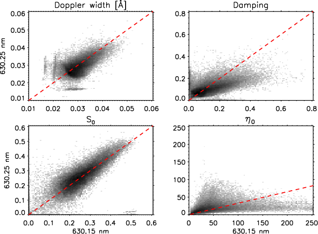
Figure 1 shows scatter plots of
![]() ,
a, S0, and
,
a, S0, and ![]() as inferred
from the inversion of the two lines. The results for S1 are very
similar to those for S0, with less scatter. In this and other
figures, the gray colors inform about the pixel density, with black
meaning higher values. Over-plotted are dashed lines representing
one-to-one correspondences, except for
as inferred
from the inversion of the two lines. The results for S1 are very
similar to those for S0, with less scatter. In this and other
figures, the gray colors inform about the pixel density, with black
meaning higher values. Over-plotted are dashed lines representing
one-to-one correspondences, except for ![]() where the ratio
where the ratio
![]() is indicated (1 and 2 stand for
the 630.15 and the 630.25 lines, respectively; see below). The plots
include all pixels in the simulation snapshot (
is indicated (1 and 2 stand for
the 630.15 and the 630.25 lines, respectively; see below). The plots
include all pixels in the simulation snapshot (
![]() ),
independently of the polarization signal. Obviously, the thermodynamic
parameters are far from being the same for the two lines. The scatter
is large for
),
independently of the polarization signal. Obviously, the thermodynamic
parameters are far from being the same for the two lines. The scatter
is large for
![]() and S0, although they show
a linear correlation with a slope close to unity. For
and S0, although they show
a linear correlation with a slope close to unity. For
![]() and a the scatter is dramatic; differences of up to a
factor 3 for a and of more than one order of magnitude for
and a the scatter is dramatic; differences of up to a
factor 3 for a and of more than one order of magnitude for ![]() can be seen. Indeed, the
can be seen. Indeed, the ![]() values obtained for
the 630.15 nm line span the full range of variation of the
line-to-continuum opacity ratio in real solar atmospheres
(see, e.g., Fig. 11 of Westendorp Plaza et al. 1998).
values obtained for
the 630.15 nm line span the full range of variation of the
line-to-continuum opacity ratio in real solar atmospheres
(see, e.g., Fig. 11 of Westendorp Plaza et al. 1998).
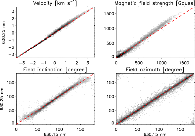
Do these discrepancies between the thermodynamic parameters affect the
magnetic and velocity inferences? The answer to this question is
negative, as can be seen in Fig. 2, where
![]() ,
B,
,
B, ![]() ,
and
,
and ![]() are displayed as
inferred from the individual inversion of the 630.15 and 630.25 nm
lines. Despite the strong scatter in the thermodynamics, the results
from both lines are remarkably similar. Therefore, we have to conclude
that although the thermodynamic parameters of ME inversions may have
little meaning, it is possible to establish approximate relations
between the parameters of the two lines for use in simultaneous
inversions, as we shall see in the next section.
are displayed as
inferred from the individual inversion of the 630.15 and 630.25 nm
lines. Despite the strong scatter in the thermodynamics, the results
from both lines are remarkably similar. Therefore, we have to conclude
that although the thermodynamic parameters of ME inversions may have
little meaning, it is possible to establish approximate relations
between the parameters of the two lines for use in simultaneous
inversions, as we shall see in the next section.
|
Figure 1:
|
| Open with DEXTER | |
|
Figure 2: Line-of-sight velocity, magnetic field strength, inclination, and azimuth from the inversion of the 630.25 nm line vs those from the inversion of the line at 630.15 nm. Both lines are inverted separately. |
| Open with DEXTER | |
3 Understanding the simultaneous inversion
Since iron is mostly ionized and local thermodynamic equilibrium
conditions prevail in the solar photosphere, the dependence of the
logarithmic derivative of ![]() on temperature (the most
important quantity in line formation) is linear with the excitation
potential
on temperature (the most
important quantity in line formation) is linear with the excitation
potential ![]() and the ionization potential I, and quadratic with
the temperature.
and the ionization potential I, and quadratic with
the temperature.
![]() is proportional to the
square root of temperature and does not depend on the atomic
parameters of the line. Assuming van der Waals broadening for the
calculation of the damping coefficient, an intricate (but weak)
dependence of a on
is proportional to the
square root of temperature and does not depend on the atomic
parameters of the line. Assuming van der Waals broadening for the
calculation of the damping coefficient, an intricate (but weak)
dependence of a on ![]() ,
along with a proportionality with the
7/10-th power of temperature, is obtained (see,
e.g., Gray 2008).
,
along with a proportionality with the
7/10-th power of temperature, is obtained (see,
e.g., Gray 2008).
|
Figure 3:
|
| Open with DEXTER | |
Neglecting the differences induced by the slightly different
excitation potentials of both lines, the a and
![]() ratios are proportional to
ratios are proportional to
![]() .
Thus, the damping and Doppler width can
safely be assumed to be equal for both lines, which is also the case for S0and S1, because the Planck function should not present significant
differences in such a short wavelength interval.
.
Thus, the damping and Doppler width can
safely be assumed to be equal for both lines, which is also the case for S0and S1, because the Planck function should not present significant
differences in such a short wavelength interval. ![]() is
proportional to the square of the central wavelength of the line and
to its gf value. Therefore,
is
proportional to the square of the central wavelength of the line and
to its gf value. Therefore,
![]() ), where g is the multiplicity of the lower
level and f the oscillator strength. Note that this ratio is
independent of the temperature or other thermodynamic quantities, so
it should not change with height in the atmosphere even if the opacity
varies by orders of magnitude. With the parameters of Table 1, the
opacity ratio for the Fe I 630 nm lines turns out to be
), where g is the multiplicity of the lower
level and f the oscillator strength. Note that this ratio is
independent of the temperature or other thermodynamic quantities, so
it should not change with height in the atmosphere even if the opacity
varies by orders of magnitude. With the parameters of Table 1, the
opacity ratio for the Fe I 630 nm lines turns out to be
![]() .
This is the value implemented in
MILOS. The HAO code and MELANIE use similar ratios
.
This is the value implemented in
MILOS. The HAO code and MELANIE use similar ratios![]() .
.
|
Figure 4:
Magnetic field strength, inclination, azimuth, and LOS velocity from
the the inversion of the 630.25 nm line vs those from the
simultaneous inversion of the two lines. The latter inversion was done
assuming the same model atmosphere (total of nine free parameters) for
the two lines, with their |
| Open with DEXTER | |
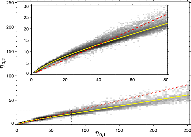
To check the validity of this estimate, we inverted the 630.25 nm line
again but forcing S0, S1,
![]() ,
and
a to be equal to those obtained from the previous inversion of the
630.15 nm line. The remaining model parameters were allowed to vary
freely. Figure 3 shows the
,
and
a to be equal to those obtained from the previous inversion of the
630.15 nm line. The remaining model parameters were allowed to vary
freely. Figure 3 shows the ![]() values retrieved
from the inversion. The dashed line represents the ratio
values retrieved
from the inversion. The dashed line represents the ratio
![]() .
The solid line corresponds to a
multi-polynomial fit
y = a[1]x3 + a[2]x2+ a[3]x with
.
The solid line corresponds to a
multi-polynomial fit
y = a[1]x3 + a[2]x2+ a[3]x with
![]() ,
,
![]() for
for
![]() and
y = b[1]x + b[2] with
b = [ 0.23,4.1] for
and
y = b[1]x + b[2] with
b = [ 0.23,4.1] for
![]() .
Note that the theoretical ratio provides a fair
description of the relationship between the two
.
Note that the theoretical ratio provides a fair
description of the relationship between the two ![]() values in
the range where most of the points are located (to stress the
differences, the inset zooms in on the boxed area). Since the exact
values of the thermodynamical parameters are not very important for
the determination of the magnetic field vector and the LOS velocity,
we conclude that it is safe to use a constant opacity ratio to invert
the two lines simultaneously without increasing the number of free
parameters.
values in
the range where most of the points are located (to stress the
differences, the inset zooms in on the boxed area). Since the exact
values of the thermodynamical parameters are not very important for
the determination of the magnetic field vector and the LOS velocity,
we conclude that it is safe to use a constant opacity ratio to invert
the two lines simultaneously without increasing the number of free
parameters.
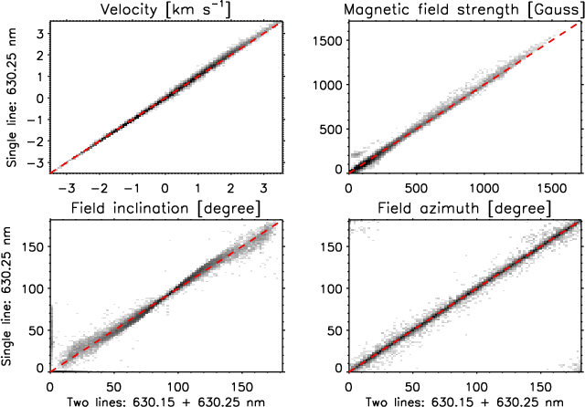
The final consistency proof is shown in Fig. 4,
where the parameters obtained from the inversion of Fe I
630.25 nm are plotted against those coming from the simultaneous
inversion of the two lines as coupled through their theoretical
![]() ratio. The scatter is very small for B and v
ratio. The scatter is very small for B and v
![]() and somewhat larger for
and somewhat larger for ![]() and
and ![]() ,
but still much smaller
than that of Fig. 2. This suggests that the accuracy of analyses based on one single line (e.g., Bommier et al. 2009) could be improved by adding the other line.
,
but still much smaller
than that of Fig. 2. This suggests that the accuracy of analyses based on one single line (e.g., Bommier et al. 2009) could be improved by adding the other line.
We thank an anonymous referee for raising the issue investigated in this paper. Our work has been supported by the Spanish MICINN through projects AYA2009-14105-C06-06 and PCI2006-A7-0624, by Junta de Andalucía through project P07-TEP-2687 (including European FEDER funds), and by the Japan Society for the Promotion of Science.
References
- Auer, L. H., House, L. L., & Heasley, J. N. 1977, Sol. Phys., 55, 47 [NASA ADS] [CrossRef] [Google Scholar]
- Bard, A., Kock, A., & Kock, M. 1991, A&A, 248, 315 [NASA ADS] [Google Scholar]
- Bommier, V., Martínez González, M., Bianda, M., et al. 2009, A&A, 506, 1415 [NASA ADS] [CrossRef] [EDP Sciences] [Google Scholar]
- Borrero, J. M., & Bellot Rubio, L. R. 2002, A&A, 385, 1056 [NASA ADS] [CrossRef] [EDP Sciences] [Google Scholar]
- Borrero, J. M., Tomczyk, S., Kubo, M., et al. 2010, Sol. Phys., 35 [Google Scholar]
- Elmore, D. F., Lites, B. W., Tomczyk, S., et al. 1992, Proc. SPIE, 1746, 22 [NASA ADS] [CrossRef] [Google Scholar]
- Gray, D. F. 2008, The Observation and Analysis of Stellar Photospheres (Cambridge: Cambridge University Press) [Google Scholar]
- Harvey, J., Livingston, W., & Slaughter, C. 1972, Line Formation in the Presence of Magnetic Fields, 227 [Google Scholar]
- Kosugi, T., Matsuzaki, K., & Sakao, T., et al. 2007, Sol. Phys., 243, 3 [NASA ADS] [CrossRef] [Google Scholar]
- Lagg, A., Woch, J., Krupp, N., & Solanki, S. K. 2004, A&A, 414, 1109 [NASA ADS] [CrossRef] [EDP Sciences] [Google Scholar]
- Landi Degl'Innocenti, E., & Landolfi, M. 1983, Sol. Phys., 87, 221 [NASA ADS] [Google Scholar]
- Landolfi, M., & Landi Degl'Innocenti, E. 1982, Sol. Phys., 78, 355 [NASA ADS] [CrossRef] [Google Scholar]
- Landolfi, M., Landi Degl'Innocenti, E., & Arena, P. 1984, Sol. Phys., 93, 269 [NASA ADS] [CrossRef] [Google Scholar]
- Lites, B. W., & Skumanich, A. 1990, ApJ, 348, 747 [NASA ADS] [CrossRef] [Google Scholar]
- Lites, B. W., Skumanich, A., Rees, D. E., & Murphy, G. A. 1988, ApJ, 330, 493 [NASA ADS] [CrossRef] [Google Scholar]
- Lites, B. W., Elmore, D. F., Seagraves, P., & Skumanich, A. P. 1993, ApJ, 418, 928 [NASA ADS] [CrossRef] [Google Scholar]
- Lites, B. W., Martinez Pillet, V., & Skumanich, A. 1994, Sol. Phys., 155, 1 [NASA ADS] [CrossRef] [Google Scholar]
- Lites, B. W., Elmore, D. F., Streander, K. V., et al. 2007, ASP Conf. Series, 369, 55 [NASA ADS] [Google Scholar]
- Martínez González, M. J., Collados, M., & Ruiz Cobo, B. 2006, A&A, 456, 1159 [NASA ADS] [CrossRef] [EDP Sciences] [Google Scholar]
- Orozco Suárez, D., & Del Toro Iniesta, J. C. 2007, A&A, 462, 1137 [NASA ADS] [CrossRef] [EDP Sciences] [Google Scholar]
- Orozco Suárez, D., Bellot Rubio, L. R., Vögler, A., & Del Toro Iniesta, J. C. 2010, A&A, 518, A2 [Google Scholar]
- Rachkovsky, D. N. 1962a, Izv. Krymsk. Astrofiz. Obs., 27, 148 [Google Scholar]
- Rachkovsky, D. N. 1962b, Izv. Krymsk. Astrofiz. Obs., 28, 259 [Google Scholar]
- Ruiz Cobo, B., & Del Toro Iniesta, J. C. 1992, ApJ, 398, 375 [NASA ADS] [CrossRef] [Google Scholar]
- Skumanich, A., & Lites, B. W. 1987, ApJ, 322, 473 [Google Scholar]
- Socas-Navarro, H. 2001, ASP Conf. Ser., 236, 487 [NASA ADS] [Google Scholar]
- Tsuneta, S., Ichimoto, K., Katsukawa, Y., et al. 2008, Sol. Phys., 249, 167 [NASA ADS] [CrossRef] [Google Scholar]
- Unno, W. 1956, PASJ, 8, 108 [NASA ADS] [Google Scholar]
- Vögler, A. 2003, Ph.D. Thesis, University of Göttingen, Germany, http://webdoc.sub.gwdg.de/diss/2004/voegler/ [Google Scholar]
- Vögler, A., Shelyag, S., Schüssler, M., et al. 2005, A&A, 429, 335 [NASA ADS] [CrossRef] [EDP Sciences] [Google Scholar]
- Westendorp Plaza, C., Del Toro Iniesta, J. C., Ruiz Cobo, B., et al. 1998, ApJ, 494, 453 [NASA ADS] [CrossRef] [Google Scholar]
Footnotes
- ... ratios
![[*]](/icons/foot_motif.png)
- The opacity ratio depends basically upon f,
which is known with limited precision and varies from one source to the
next. This causes an uncertainty in the theoretical opacity ratio. For
example, the laboratory measurements of Bard et al. 1991
give
 for Fe I 630.15 nm, rather than
the -0.75 specified in Table 1. With this oscillator strength,
the theoretical ratio would be 0.301 (closer to the values retrieved
from the inversion, but only at the high
for Fe I 630.15 nm, rather than
the -0.75 specified in Table 1. With this oscillator strength,
the theoretical ratio would be 0.301 (closer to the values retrieved
from the inversion, but only at the high  end).
end).
All Tables
Table 1: Atomic data for the Fe I 630 nm lines.
All Figures
|
|
Figure 1:
|
| Open with DEXTER | |
| In the text | |
|
|
Figure 2: Line-of-sight velocity, magnetic field strength, inclination, and azimuth from the inversion of the 630.25 nm line vs those from the inversion of the line at 630.15 nm. Both lines are inverted separately. |
| Open with DEXTER | |
| In the text | |
|
|
Figure 3:
|
| Open with DEXTER | |
| In the text | |
|
|
Figure 4:
Magnetic field strength, inclination, azimuth, and LOS velocity from
the the inversion of the 630.25 nm line vs those from the
simultaneous inversion of the two lines. The latter inversion was done
assuming the same model atmosphere (total of nine free parameters) for
the two lines, with their |
| Open with DEXTER | |
| In the text | |
Copyright ESO 2010
Current usage metrics show cumulative count of Article Views (full-text article views including HTML views, PDF and ePub downloads, according to the available data) and Abstracts Views on Vision4Press platform.
Data correspond to usage on the plateform after 2015. The current usage metrics is available 48-96 hours after online publication and is updated daily on week days.
Initial download of the metrics may take a while.