| Issue |
A&A
Volume 518, July-August 2010
Herschel: the first science highlights
|
|
|---|---|---|
| Article Number | A2 | |
| Number of page(s) | 11 | |
| Section | The Sun | |
| DOI | https://doi.org/10.1051/0004-6361/200913421 | |
| Published online | 18 August 2010 | |
Applicability of Milne-Eddington
inversions to high spatial resolution observations of the quiet Sun![[*]](/icons/foot_motif.png)
D. Orozco Suárez1,2 - L. R. Bellot Rubio1 - A. Vögler3 - J. C. del Toro Iniesta1
1 - Instituto de Astrofísica de Andalucía (CSIC),
Apdo. Correos 3004, 18080 Granada, Spain
2 - National Astronomical Observatory of Japan, 2-21-1 Osawa, Mitaka,
Tokyo 181-8588, Japan
3 - Sterrenkundig Instituut, Utrecht University, Postbus 80000, 3508 TA
Utrecht, The Netherlands
Received 8 October 2009 / Accepted 26 May 2010
Abstract
Context. The physical conditions of the solar
photosphere change on very small spatial scales both horizontally and
vertically. Such a complexity may pose a serious obstacle to the
accurate determination of solar magnetic fields.
Aims. We examine the applicability of
Milne-Eddington (ME) inversions to high spatial resolution observations
of the quiet Sun. Our aim is to understand the connection between the
ME inferences and the actual stratifications of the atmospheric
parameters.
Methods. We use magnetoconvection simulations of the
solar surface to synthesize asymmetric Stokes profiles such as those
observed in the quiet Sun. We then invert the profiles with the
ME approximation. We perform an empirical analysis of the
heights of formation of ME measurements and analyze the
uncertainties brought about by the ME approximation. We also
investigate the quality of the fits and their relationship with the
model stratifications.
Results. The atmospheric parameters derived from ME
inversions of high-spatial resolution profiles are reasonably accurate
and can be used for statistical analyses of solar magnetic fields, even
if the fit is not always good. We also show that the ME inferences
cannot be assigned to a specific atmospheric layer: different
parameters sample different ranges of optical depths, and even the same
parameter may trace different layers depending on the physical
conditions of the atmosphere. Despite this variability,
ME inversions tend to probe deeper layers in granules than in
intergranular lanes.
Key words: magnetic fields - instrumentation: high angular resolution - Sun: photosphere
1 Introduction
The solar spectrum carries information about the properties of our star. In general, a broad range of atmospheric layers contribute to the shape of the spectral lines, making it difficult to extract this information directly. Both the measurement process and the method of analysis introduce uncertainties in the physical quantities retrieved from the observations. Sources of error are photon noise and instrumental effects such as limited spectral resolution, wavelength sampling, and angular resolution, but also the simplifications and approximations of the model used to interpret the measurements.
In this paper we evaluate the merits of Milne-Eddington (ME) inversions for the analysis of the polarization line profiles emerging from the solar atmosphere. The ME approximation does not account for vertical variations of the parameters (Rachkovsky 1962,1967; Unno 1956), so it cannot accurately describe the solar plasma when rapid changes in height are present. What then is the significance of the ME parameters?
To answer this question it is necessary to simulate the processes of line formation and data inversion. Usually one prescribes a set of model atmospheres, performs spectral synthesis calculations, inverts the synthetic profiles, and compares the results with the known input. A common approach is to use ME models both to generate the spectra and to invert them (e.g., Borrero et al. 2007; Norton et al. 2006). In that case the analysis is internally consistent and the uncertainties of the retrieved ME parameters are mostly due to the noise and, to a smaller extent, to the convergence of the algorithm, provided that the spectral resolution and wavelength sampling are appropriate. Uncertainties caused by photon noise are known as statistical errors and can be evaluated by means of numerical tests or, more efficiently, by using ME response functions (Del Toro Iniesta et al. 2010; Orozco Suárez & Del Toro Iniesta 2007). However, they represent only a small fraction of the total error. Another source of error is the very assumption of height-independent parameters, which leads to symmetric line profiles. What happens when realistic (i.e., asymmetric) Stokes spectra are analyzed in terms of ME models? Do the uncertainties of the retrieved parameters increase significantly? Answering these questions is the aim of the present work.
A first study of the capabilities and limitations of ME inversions was carried out by Westendorp Plaza et al. (1998) with simple (non-ME) model atmospheres. They made a quantitative comparison of results obtained with the ME code of the High Altitude Observatory (Lites & Skumanich 1990; Skumanich & Lites 1987) and the SIR code (Stokes Inversion based on Response functions, Ruiz Cobo & Del Toro Iniesta 1992). The main conclusion of their work was that ME inversions provide accurate values of the physical parameters averaged along the line of sight, at least when the stratifications are smooth.
More recently, Khomenko & Collados (2007b) have investigated whether the magnetic field stratification itself can be determined reliably through inversion of high-resolution data. To that end, they synthesized the Stokes profiles of the Fe I 630 nm lines with the help of MHD models and inverted them with SIR, allowing for vertical gradients of the atmospheric parameters. The analysis showed that SIR is able to recover the actual magnetic stratification for fields as weak as 50 G if there is no noise. This work extends the results of Westendorp Plaza et al. (1998) to the case in which the stratifications are not smooth.
To determine the uncertainties associated with ME inversions
of asymmetric Stokes profiles we use state-of-the-art
magnetohydrodynamic simulations (Sect. 2). Our goal is to
describe the solar photosphere as realistically as possible. We
construct model atmopheres from the simulations and synthesize the
emerging Stokes profiles of the Fe I 630.2 nm
lines (Sect. 3).
The SIR code is used for the spectral synthesis,
so the profiles are asymmetric. Finally, we apply an
ME inversion to the data (Sect. 4). The spatial
sampling of the MHD models ![]() is preserved in our numerical experiments. There are two reasons why we
neglect the effects of solar instrumentation: first, they have already
been studied before (e.g., Orozco
Suárez et al. 2007, 2010a,b);
second, this sampling
is close to critical for the observations to be delivered by large
telescopes like the Advanced Technology Solar Telescope
is preserved in our numerical experiments. There are two reasons why we
neglect the effects of solar instrumentation: first, they have already
been studied before (e.g., Orozco
Suárez et al. 2007, 2010a,b);
second, this sampling
is close to critical for the observations to be delivered by large
telescopes like the Advanced Technology Solar Telescope![]() (Wagner
et al. 2006) and the European Solar Telescope
(Wagner
et al. 2006) and the European Solar Telescope![]() (Collados
2008). We invert the profiles with the MILOS code (Orozco Suárez & Del
Toro Iniesta 2007)
(Collados
2008). We invert the profiles with the MILOS code (Orozco Suárez & Del
Toro Iniesta 2007)![]() .
A direct comparison of the retrieved and true parameters
allows us to determine the effective ``heights of formation'' of the
ME parameters (Sect. 5) and to quantify
the errors caused by the ME approximation (Sect. 6). The
conclusions of our work are given in Sect. 7.
For completeness, the results of ME inversions are
compared with those of tachogram/magnetogram-like analyses in
the Appendix.
.
A direct comparison of the retrieved and true parameters
allows us to determine the effective ``heights of formation'' of the
ME parameters (Sect. 5) and to quantify
the errors caused by the ME approximation (Sect. 6). The
conclusions of our work are given in Sect. 7.
For completeness, the results of ME inversions are
compared with those of tachogram/magnetogram-like analyses in
the Appendix.
2 Magnetohydrodynamic simulations
We use radiative MHD simulations performed with MURaM, the MPS/University of Chicago RAdiative MHD code (Vögler et al. 2005; Vögler 2003). This code solves the 3D time-dependent MHD equations for a compressible and partially ionized plasma taking into account non-grey radiative energy transport and opacity binning (Nordlund 1982).
|
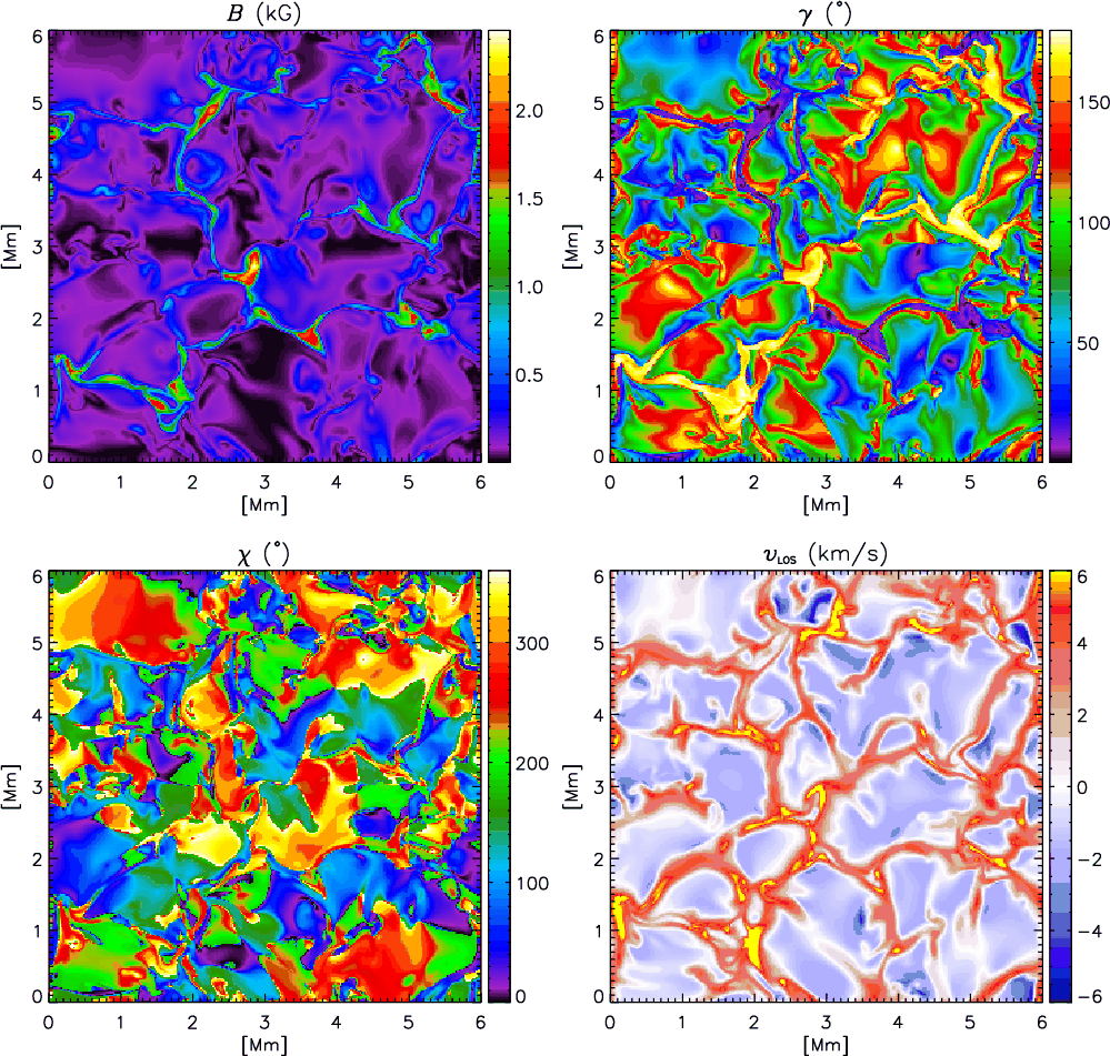
Figure 1:
Magnetic field strength, inclination, azimuth, and
LOS velocity at |
| Open with DEXTER | |
Among other problems, MURaM has been employed to study facular brightenings (Keller et al. 2004), the relation between G-band bright points and magnetic flux concentrations (Shelyag et al. 2004; Schüssler et al. 2003), the emergence of magnetic flux tubes from the upper convection zone to the photosphere (; Cheung et al. 2007), the strongly inclined magnetic fields of the internetwork (Schüssler & Vögler 2008), umbral dots (Schüssler & Vögler 2006), solar pores (Cameron et al. 2007), and even full sunspots (Rempel et al. 2009a,b). MURaM has also been used to evaluate the diagnostic potential of spectral lines (Shelyag et al. 2007; Khomenko et al. 2005a; Khomenko & Collados 2007b,a; Khomenko et al. 2005b), the validity of visible lines for the study of internetwork magnetic fields at high spatial resolution (Orozco Suárez et al. 2007), and the continuum contrast of the solar granulation (Danilovic et al. 2008).
In this paper we consider a 5-min sequence of a mixed-polarity
simulation run representing a network region with an average magnetic
field strength ![]() G
at
G
at ![]()
![]() .
The cadence is 10 s, so we have
30 snapshots. A bipolar distribution of vertical
fields with
.
The cadence is 10 s, so we have
30 snapshots. A bipolar distribution of vertical
fields with ![]() G
was used to initialize the simulations. Additional details about this
particular run can be found in Khomenko
et al. (2005a).
G
was used to initialize the simulations. Additional details about this
particular run can be found in Khomenko
et al. (2005a).
The computational box has 288 ![]() 288
288 ![]() 100 grid points and covers 6000 km in the horizontal
direction and 1400 km in the vertical direction. The model
extends from z=-800 to z=600 km,
with z=0 km the average of the heights
where
100 grid points and covers 6000 km in the horizontal
direction and 1400 km in the vertical direction. The model
extends from z=-800 to z=600 km,
with z=0 km the average of the heights
where ![]() .
The spatial grid sampling is 0
.
The spatial grid sampling is 0
![]() 0287,
implying an equivalent resolution of 0
0287,
implying an equivalent resolution of 0
![]() 057
(41.6 km) on the solar surface. The
simulation provides the density, the linear momentum density
vector, the total energy density, the magnetic field vector,
the temperature, and the gas pressure at every grid point. The
time-averaged radiation flux density leaving the top of the box has the
solar value
057
(41.6 km) on the solar surface. The
simulation provides the density, the linear momentum density
vector, the total energy density, the magnetic field vector,
the temperature, and the gas pressure at every grid point. The
time-averaged radiation flux density leaving the top of the box has the
solar value ![]()
![]() 1010 erg s-1 cm-2.
1010 erg s-1 cm-2.
3 Spectral synthesis
In order to compute synthetic Stokes profiles we solve the radiative transfer equation (RTE) for polarized light. The calculations are carried out with the SIR code with the opacity routines of Wittmann (1974). The spectral synthesis is accomplished in two steps: first, the input model atmospheres are built from the MHD simulations; then, the RTE is solved.
3.1 MHD models and spectral line synthesis
The parameters needed for the spectral synthesis are the temperature,
electron pressure, line-of-sight (LOS) velocity, magnetic field
strength, inclination and azimuth, and optical depth. The simulations
provide most of them. However, the electron pressure and optical depth
need to be computed from the local temperature, gas pressure, and
density by solving the Saha and Boltzmann equations. The optical depth
scale is set up assuming that z=600 km
(the top of the computational box) corresponds to ![]() .
This value has been taken from the Harvard-Smithsonian Reference
Atmosphere (HSRA, Gingerich
et al. 1971). Finally, the resulting stratifications
are interpolated to an evenly spaced optical depth grid using
second-order polynomials. The grid extends from
.
This value has been taken from the Harvard-Smithsonian Reference
Atmosphere (HSRA, Gingerich
et al. 1971). Finally, the resulting stratifications
are interpolated to an evenly spaced optical depth grid using
second-order polynomials. The grid extends from ![]() to 2 with
to 2 with ![]() .
This range of optical depths encompasses
the formation region of all photospheric lines, except the cores of the
strongest ones.
.
This range of optical depths encompasses
the formation region of all photospheric lines, except the cores of the
strongest ones.
Figure 1
displays maps of the field strength, inclination, azimuth, and LOS
velocity at ![]() for one simulation snapshot. In the velocity map the
granulation pattern is clearly visible, with granular upflows that are
weaker than the intergranular downflows. Some of the small-scale
intergranular structures have velocities of up to 6
for one simulation snapshot. In the velocity map the
granulation pattern is clearly visible, with granular upflows that are
weaker than the intergranular downflows. Some of the small-scale
intergranular structures have velocities of up to 6
![]() .
.
The field strength map shows strong flux concentrations in the
intergranular lanes. Granules also harbor magnetic fields, but they
seldom exceed 300 G. There is a tight correlation between the
field strength and inclination in these simulations: the intergranular
fields tend to be vertical, whereas the granules exhibit more
horizontal fields. Finally, the azimuth map is dominated by
granular-sized structures with diameters of 1
![]() -2
-2
![]() (0.7-1.5 Mm).
(0.7-1.5 Mm).
![\begin{figure}
\par\includegraphics[width=8cm,clip]{13421Fig2a.ps}\vspace*{3mm}
\includegraphics[width=8cm,clip]{13421Fig2b.ps}
\end{figure}](/articles/aa/full_html/2010/10/aa13421-09/img18.png)
|
Figure 2:
Probability density functions for the magnetic field strength and field
inclination at |
| Open with DEXTER | |
Figure 2
depicts the probability density functions (PDFs)![]() of the magnetic field strength and inclination at optical depth
of the magnetic field strength and inclination at optical depth ![]() ,
averaged over the 30 available snapshots. The field strength
PDF increases rapidly toward weak fields, indicating that most pixels
have magnetic fields of the order of hectogauss. The distribution peaks
at about 20 G. The inclination PDF shows some
vertical fields and a larger occurrence of horizontal fields. The
simulation run was seeded with mixed-polarity vertical fields;
therefore, the distribution is rather symmetric about
,
averaged over the 30 available snapshots. The field strength
PDF increases rapidly toward weak fields, indicating that most pixels
have magnetic fields of the order of hectogauss. The distribution peaks
at about 20 G. The inclination PDF shows some
vertical fields and a larger occurrence of horizontal fields. The
simulation run was seeded with mixed-polarity vertical fields;
therefore, the distribution is rather symmetric about ![]() .
.
Table 1: Atomic parameters of the spectral lines.
Once we have constructed model atmospheres for each of the
288 ![]() 288 pixels and for all the snapshots, we use them to compute
the Stokes profiles of Fe I 630.15
and 630.25 nm. The atomic parameters used in the calculations
are given in Table 1.
The
288 pixels and for all the snapshots, we use them to compute
the Stokes profiles of Fe I 630.15
and 630.25 nm. The atomic parameters used in the calculations
are given in Table 1.
The ![]() values
have been taken from the VALD database (Piskunov
et al. 1995), except for Fe I 630.25 nm
which is not available in VALD and comes from a fit to the solar
spectrum using the two-component model of Borrero
& Bellot Rubio (2002). The collisional broadening
coefficients
values
have been taken from the VALD database (Piskunov
et al. 1995), except for Fe I 630.25 nm
which is not available in VALD and comes from a fit to the solar
spectrum using the two-component model of Borrero
& Bellot Rubio (2002). The collisional broadening
coefficients ![]() and
and ![]() due to neutral hydrogen atoms have been evaluated following the
procedure of Anstee & O'Mara
(1995) and
Barklem
et al. (2000,1998). The abundances have been
taken from Thévenin (1989),
i.e., a value of 7.46 is employed
for iron.
due to neutral hydrogen atoms have been evaluated following the
procedure of Anstee & O'Mara
(1995) and
Barklem
et al. (2000,1998). The abundances have been
taken from Thévenin (1989),
i.e., a value of 7.46 is employed
for iron.
3.2 Synthesis results
Figure 3 shows a continuum map of the simulated region. The rms contrast, computed as the standard deviation divided by the mean, is 14.8% at 630 nm. This contrast exceeds the typical values obtained from ground-based observations; the speckle-reconstructed G-band images taken at the Dunn Solar Telescope, for example, show contrasts of 14.1% (Uitenbroek et al. 2007). Nevertheless, the agreement is reasonable because the observed values are degraded by instrumental effects (e.g., Danilovic et al. 2008; Wedemeyer-Böhm & Rouppe van der Voort 2009).
We have compared the temporally and spatially averaged intensity profiles with the corresponding ones in the Fourier Transform Spectrometer (FTS) atlas of the quiet Sun by Brault & Neckel (1987) and Neckel (1999, see Fig. 4). For the comparison, the simulated profiles have been first normalized to unity and then displaced in wavelength to correct for the solar gravitational redshift (see Lopresto et al. 1980). Also, an additional minor correction to the wavelength shift has been allowed to improve the fits. The figure shows that the widths of the synthetic profiles are very similar to those measured in the FTS atlas. However, the bottom panels indicate that the simulations do not completely reproduce the line asymmetries: the differences between observed and synthetic profiles are small (of the order of 2.5%), but not zero.
In summary, despite some differences between the FTS and the synthetic profiles, the simulations appear to explain the observations rather well. Therefore, we hope that they also produce sufficiently realistic polarization spectra, in particular with regard to their asymmetries.
![\begin{figure}
\par\includegraphics[width=9cm,clip]{13421Fig3.eps}
\end{figure}](/articles/aa/full_html/2010/10/aa13421-09/img33.png)
|
Figure 3: Continuum intensity map for the simulation snapshot depicted in Fig. 1. The wavelength is 630 nm. |
| Open with DEXTER | |
![\begin{figure}
\par\includegraphics[width=8.5cm,clip]{13421Fig4.ps}
\end{figure}](/articles/aa/full_html/2010/10/aa13421-09/img34.png)
|
Figure 4: Average intensity profiles from the simulations (solid) and the FTS atlas (dashed), for the Fe I lines at 630.2 nm. The bottom panel shows the intensity differences (FTS - simulation) in percent. |
| Open with DEXTER | |
4 ME inversion of the Stokes profiles
To determine the vector magnetic field and the LOS velocity we
perform ME inversions. Given the high spatial and temporal
resolution of the simulations, the macroturbulence is set to zero and
the filling factor to unity, i.e., the magnetic atmosphere is assumed
to occupy the whole pixel (one-component model atmospheres).
A total of nine quantities are determined from the inversion:
the thermodynamic parameters S0,
S1, ![]() ,
,
![]() ,
and a (representing the intercept and the
slope of the source function, the line-to-continuum opacity
ratio, the Doppler width, and the damping parameter), the strength,
inclination, and azimuth of the magnetic
field vector (B,
,
and a (representing the intercept and the
slope of the source function, the line-to-continuum opacity
ratio, the Doppler width, and the damping parameter), the strength,
inclination, and azimuth of the magnetic
field vector (B, ![]() ,
and
,
and ![]() ),
and the line-of-sight velocity (
),
and the line-of-sight velocity (
![]() ). The Stokes profiles are
taken from a single snapshot of the simulation. No noise is added to
the spectra to better isolate the uncertainties due to the
ME approximation.
). The Stokes profiles are
taken from a single snapshot of the simulation. No noise is added to
the spectra to better isolate the uncertainties due to the
ME approximation.
The Fe I lines at 630 nm
belong to the same multiplet and are formed under very similar
thermodynamic conditions. Hence, we can reliably assume that the ME
thermodynamic parameters are the same for both lines except
for ![]() .
A simultaneous inversion with no extra free parameters is thus
possible using a constant
.
A simultaneous inversion with no extra free parameters is thus
possible using a constant ![]() ratio and the same
ratio and the same
![]() and a values for the two lines. This is
the strategy implemented in several ME codes (for details, see
Orozco Suárez et al. 2010b).
and a values for the two lines. This is
the strategy implemented in several ME codes (for details, see
Orozco Suárez et al. 2010b).
We use the same initial guess model for all the pixels,
stopping the inversion when convergence is achieved or
200 iterations have been performed. The initial model is given
by S0=0.2, S1=0.8,
![]() ,
,
![]() mÅ,
a=0.03, B=200 G,
mÅ,
a=0.03, B=200 G, ![]()
![]() ,
,
![]()
![]() ,
and
,
and ![]()
![]() .
.
5 Understanding ME inferences
![\begin{figure}
\par\includegraphics[width=17cm,clip]{13421Fig5.eps}
\vspace*{2mm}
\end{figure}](/articles/aa/full_html/2010/10/aa13421-09/img46.png)
|
Figure 5: Examples of MHD atmospheres and simulated profiles (black) and ME fits (red) for three different pixels. Left panels: magnetic field strength, inclination, azimuth, and LOS velocity stratifications. The red horizontal lines indicate the inversion results. Right panels: Stokes I, Q, U and V profiles synthesized from the MHD simulations without noise (black) and ME fits (red). Cases a)- c) correspond to (x,y) = (1.75, 1.08), (2.90, 2.58), and (1.67, 1.73) Mm in Figs. 6 and 7. |
| Open with DEXTER | |
The line asymmetries observed in the solar atmosphere imply that there are vertical gradients of the physical parameters, because the line wings trace relatively deep layers and the core is formed higher in the atmosphere. By contrast, the ME fits are strictly symmetric and deliver height-independent atmospheric parameters. Thus, it is important to verify that the ME model can indeed be used for the analysis of observations at very high spatial resolution.
Figure 5 shows the magnetic field strength, inclination, azimuth, and LOS velocity stratifications in three pixels of the simulation snapshot, labeled (a)-(c). The figure also displays the corresponding Stokes I, Q, U, and V profiles. The results of the ME inversions are overplotted in red. Case (a) shows symmetric Stokes profiles, in (b) the profiles are rather asymmetric, and (c) shows three-lobed Stokes V spectra together with anomalous linear polarization signals. (a) represents a strong field case and (b) and (c) correspond to weak fields. In the three examples the atmospheric quantities undergo large variations with optical depth.
The ME fit is good in (a) and worse in (b) and (c). Clearly, as the asymmetry level increases, the ME model has more difficulties to reproduce the profiles. The misfits are obvious in Stokes Q, U, and V, and less dramatic in Stokes I.
The models retrieved from the inversion are shown in the left panels of Fig. 5 (red lines). The height-independent ME parameters can be interpreted as averages of the actual stratifications weighted by the corresponding response functions (Westendorp Plaza et al. 1998). In general it is difficult to confirm this by simply looking at the atmospheric stratifications, but case (c) provides a particularly clear example. This case represents a pixel whose ME fit is not satisfactory. The analysis of the stratifications shows that the profiles arise from an atmosphere that has sharp discontinuities in field strength, inclination, azimuth, and LOS velocity, located more or less at the same optical depth. The two parts of the atmosphere separated by the discontinuity leave clear signatures in the emergent Stokes V spectra, to the point that the magnetic and kinematic properties of the plasma above and below the discontinuity can roughly be guessed from a simple inspection of the profiles: there is a weak field associated with small velocites and a stronger field showing large redshifts. Surprisingly, however, the ME model returned by the inversion seems to describe only the weak field.
To understand why this happens, it is important to realize that the inversion algorithm uses all the wavelength samples to determine the best-fit ME parameters. As mentioned before, different wavelength positions across the line trace different atmospheric layers. Thus, the ME inversion is forced to return average parameters along the LOS in order to fit the whole line profile reasonably well without any bias toward better fits in the core or the wings. This favors the weak field component of the atmosphere because it occupies most of the line-forming region in this particular example.
![\begin{figure}
\par\hspace*{1.5mm}\includegraphics[width=8cm,clip]{13421Fig6a.ps...
...ps}\hspace*{5mm}
\includegraphics[width=7.85cm,clip]{13421Fig6d.ps}
\end{figure}](/articles/aa/full_html/2010/10/aa13421-09/img47.png)
|
Figure 6: Top: optical depths at which the inferred ME parameters coincide with the real magnetic field strength and LOS velocity stratifications (left and right, respectively). Bottom: magnetic field strengths retrieved from the ME inversion and normalized continuum intensities (left and right, respectively). |
| Open with DEXTER | |
Figure 5 demonstrates that the ME model parameters coincide with the real stratifications at specific optical depths. This allows us to define the effective ``height of formation'' of the ME parameters.
Formation-height maps have been calculated by taking the
optical depth at which the stratification is closer to the inferred
ME parameter. The formation heights are constrained to be in
the range from ![]() to -2 because this interval includes most of the layers to
which the Fe I lines are
sensitive. When more than one value of the MHD stratification coincides
with the corresponding ME parameter, we select the one located
deeper in the atmosphere. The optical depth of the minimum
(or maximum) of the MHD stratification is taken if
the ME parameter is smaller (or larger) than all
stratification values. Even then the formation height is not allowed to
go outside of the interval from
to -2 because this interval includes most of the layers to
which the Fe I lines are
sensitive. When more than one value of the MHD stratification coincides
with the corresponding ME parameter, we select the one located
deeper in the atmosphere. The optical depth of the minimum
(or maximum) of the MHD stratification is taken if
the ME parameter is smaller (or larger) than all
stratification values. Even then the formation height is not allowed to
go outside of the interval from ![]() to -2.
to -2.
Figure 6
shows the results for the magnetic field strength and the
LOS velocity. For convenience, we also display the
continuum image and the field strengths retrieved from the inversion.
Different colors indicate different atmospheric layers. There are clear
differences between the two maps: the granular centers are
predominantly green (
![]() )
in the velocity map and green-red (
)
in the velocity map and green-red (
![]() )
in the field strength map, demonstrating that the ME inversion
extracts the velocities from higher optical depths than the magnetic
fields, at least in granules. The intergranular lanes tend to
show blue colors in the two maps (
)
in the field strength map, demonstrating that the ME inversion
extracts the velocities from higher optical depths than the magnetic
fields, at least in granules. The intergranular lanes tend to
show blue colors in the two maps (
![]() ).
The sharp red-yellow discontinuities observed at the border of granules
in the velocity map have little meaning since they are a result of the
way we estimate formation
heights. These regions have zero velocities (Fig. 1) and also zero
velocity gradients along the LOS, which makes our algorithm select
layers close to the bottom of the photosphere (limited to
).
The sharp red-yellow discontinuities observed at the border of granules
in the velocity map have little meaning since they are a result of the
way we estimate formation
heights. These regions have zero velocities (Fig. 1) and also zero
velocity gradients along the LOS, which makes our algorithm select
layers close to the bottom of the photosphere (limited to ![]() ). Both maps
exhibit significant pixel-to-pixel differences, especially the
field-strength map. This ``noise'' is caused by
MHD stratifications with many jumps in the vertical
direction.
). Both maps
exhibit significant pixel-to-pixel differences, especially the
field-strength map. This ``noise'' is caused by
MHD stratifications with many jumps in the vertical
direction.
In summary, ME inversions provide results that cannot be
assigned to a constant optical depth. The same parameter may show
formation-height differences of up to 1-1.5 dex across the
FOV. Also, the heights to which the ME parameters refer change
depending on the parameter, as predicted by Del Toro Iniesta & Ruiz
Cobo (1996) and Sánchez
Almeida et al. (1996). In the case of the Fe I 630.2 nm
lines, we find mean optical depths of ![]() and -1.1 for the LOS velocity and the field strength,
respectively. This includes granular and intergranular regions. If only
intergranular regions are considered, the mean optical depths move
and -1.1 for the LOS velocity and the field strength,
respectively. This includes granular and intergranular regions. If only
intergranular regions are considered, the mean optical depths move ![]() 0.2 dex
toward higher layers. The rms variation of the formation heights
is 0.4 and 0.5 dex, respectively.
0.2 dex
toward higher layers. The rms variation of the formation heights
is 0.4 and 0.5 dex, respectively.
6 Inversion results
Below we compare the ME inversion results with the original
MHD models. To that end we use the atmospheric
parameters of the simulations at ![]() .
This layer corresponds to the average
formation height of the ME parameters. As such,
it represents the best choice for a ``reference model''.
.
This layer corresponds to the average
formation height of the ME parameters. As such,
it represents the best choice for a ``reference model''.
Figure 7 displays maps of the magnetic field strength, inclination, azimuth, and LOS velocity in the reference model (left column) and the models retrieved from the inversion (right column). To better visualize the details we only show a small area of about 9 Mm2. The strong resemblance between the reference parameters and the ME models is obvious: the shapes of the different structures are well reproduced and only small differences can be recognized. Sometimes the inversion yields bad results for the inclination and azimuth, but this happens mainly in areas with weak polarization signals.
From a visual inspection of the maps, one can say that the
ME inversion is able to determine the magnetic field vector
satisfactorily. Even structures with field strengths as low as
100 G are well recovered. To make more precise
statements, Fig. 8
shows the parameters inferred from the fit vs. the MHD
parameters at ![]() .
These scatter plots allow us to estimate the uncertainties that can be
expected from the use of the ME approximation, since no noise
has been added to the profiles (Sect. 4).
.
These scatter plots allow us to estimate the uncertainties that can be
expected from the use of the ME approximation, since no noise
has been added to the profiles (Sect. 4).
![\begin{figure}
\par\includegraphics[width=8.8cm,clip]{13421Fig7.eps}
\end{figure}](/articles/aa/full_html/2010/10/aa13421-09/img54.png)
|
Figure 7:
From top to bottom: magnetic field strength,
inclination, azimuth, and LOS velocity. The left
column represents the MHD parameters at |
| Open with DEXTER | |
![\begin{figure}
\par\includegraphics[width=9cm,clip]{13421Fig8.eps}
\end{figure}](/articles/aa/full_html/2010/10/aa13421-09/img55.png)
|
Figure 8:
Scatter plots of the magnetic field strength, inclination, azimuth and
LOS velocity inferred from the
ME inversion vs. the MHD parameters at |
| Open with DEXTER | |
As can be seen, the scatter is larger for the magnetic field
inclination and azimuth. The mean values of the parameters![]() (red dots) show that the
magnetic field strength is really close to that in the reference model
from 0 to 500 G. For stronger
fields the retrieved values are slightly underestimated, although the
deviation does not exceed
(red dots) show that the
magnetic field strength is really close to that in the reference model
from 0 to 500 G. For stronger
fields the retrieved values are slightly underestimated, although the
deviation does not exceed ![]() 250 G.
The red lines indicate maximum rms fluctuations of about
250 G.
The red lines indicate maximum rms fluctuations of about ![]() 80 G
in the whole range of strengths. The inclination shows rms fluctuations
smaller than 10
80 G
in the whole range of strengths. The inclination shows rms fluctuations
smaller than 10
![]() for vertical fields and 15
for vertical fields and 15
![]() for inclined fields. The rms variation in the azimuth is about 15
for inclined fields. The rms variation in the azimuth is about 15
![]() .
The LOS velocity panel shows that the retrieved velocity is
some 200-300
.
The LOS velocity panel shows that the retrieved velocity is
some 200-300
![]() lower than the reference velocities for receding flows (intergranular
lanes). The rms values are lower than
lower than the reference velocities for receding flows (intergranular
lanes). The rms values are lower than ![]() 500
500
![]() in the full velocity range.
in the full velocity range.
The scatter observed in the various panels of Fig. 8 originates from the
use of ME model atmospheres (unable to fit asymmetric Stokes
profiles) and the pixel-to-pixel variations of the
formation height of the ME parameters, as explained
in the previous section. The deviation of the ME field
strengths from a one-to-one correspondence with the MHD models
can easily be understood by looking at the top panel of Fig. 6 and recalling that
we have chosen the atmospheric layer at ![]() as a reference. In those spatial locations where the optical
depth assigned to the retrieved ME parameter is smaller than
the optical depth of the reference layer, the resulting field
strength will ``apparently'' be underestimated. These spatial locations
are associated with strong
flux concentrations; in the MHD models they spread out with
height, therefore we retrieve weaker fields.
as a reference. In those spatial locations where the optical
depth assigned to the retrieved ME parameter is smaller than
the optical depth of the reference layer, the resulting field
strength will ``apparently'' be underestimated. These spatial locations
are associated with strong
flux concentrations; in the MHD models they spread out with
height, therefore we retrieve weaker fields.
The rms differences between the inversion results and the MHD models tell us how much a single ME parameter could deviate from the real value, but only if the mean differences are zero or close to zero. Non-zero mean differences indicate that systematic errors exist. For this reson, when the mean difference is larger than the standard deviation, the former should be preferred as a better estimate of the true error.
The choice of ![]() for the reference model is appropriate because it produces the lower
mean and rms values on average. To illustrate this,
Fig. 9
represents histograms of the
differences between the inferred parameters and the MHD model
at three optical depths (
for the reference model is appropriate because it produces the lower
mean and rms values on average. To illustrate this,
Fig. 9
represents histograms of the
differences between the inferred parameters and the MHD model
at three optical depths (![]() =
-0.5,-1,-1.5, coded in black,
red, and green, respectively).
=
-0.5,-1,-1.5, coded in black,
red, and green, respectively).
![\begin{figure}
\par\includegraphics[width=8.8cm,clip]{13421Fig9.eps}
\end{figure}](/articles/aa/full_html/2010/10/aa13421-09/img58.png)
|
Figure 9: Normalized histograms of the differences between the inferred ME model parameters and the real ones taken at different optical depths. |
| Open with DEXTER | |
For the magnetic field strength, the histogram corresponding to ![]() peaks
around zero. The maximum shifts toward negative values when the
inversion results are compared with deeper layers
(fields are underestimated on average) and toward positive values when
the comparison is made with higher layers (over-estimating the
strength). The full width at half maximum (FWHM) of
the distribution is about 30 G for
peaks
around zero. The maximum shifts toward negative values when the
inversion results are compared with deeper layers
(fields are underestimated on average) and toward positive values when
the comparison is made with higher layers (over-estimating the
strength). The full width at half maximum (FWHM) of
the distribution is about 30 G for ![]() ,
and increases up to
,
and increases up to ![]() 45
and
45
and ![]() 50 G
for
50 G
for ![]() and -0.5, respectively. These effects are less pronounced for
the field inclination: the peaks of the histograms are located
at zero and the FWHM varies from 6
and -0.5, respectively. These effects are less pronounced for
the field inclination: the peaks of the histograms are located
at zero and the FWHM varies from 6
![]() (
(
![]() )
to
)
to ![]() 13
13
![]() and
and
![]() 23
23
![]() (
(
![]() and -0.5, respectively). The larger FWHMs
originate from the extended wings of the distributions. The azimuth
histogram does not vary when the comparison is made with different
optical depths. Then the FWHM is about 20
and -0.5, respectively). The larger FWHMs
originate from the extended wings of the distributions. The azimuth
histogram does not vary when the comparison is made with different
optical depths. Then the FWHM is about 20
![]() .
.
The histograms of the LOS velocity differences show larger
variations. The one corresponding to ![]() has the smaller FWHM (
has the smaller FWHM (![]()
![]() ).
It also features a long tail toward negative values caused by
pixels located in intergranular lanes. The asymmetry of the histograms
around the location of the peaks changes dramatically when we compare
the inversion results with different atmospheric layers.
For instance, if the reference layer is taken at
).
It also features a long tail toward negative values caused by
pixels located in intergranular lanes. The asymmetry of the histograms
around the location of the peaks changes dramatically when we compare
the inversion results with different atmospheric layers.
For instance, if the reference layer is taken at ![]() ,
the histogram is a clear combination of two different distributions,
one representing granular centers (higher and narrower) and the other
representing intergranular lanes (smaller in amplitude and broader).
,
the histogram is a clear combination of two different distributions,
one representing granular centers (higher and narrower) and the other
representing intergranular lanes (smaller in amplitude and broader).
7 Summary and conclusions
We have analyzed radiative MHD simulations of the quiet Sun. We have
used them to synthesize Stokes line profiles in three different
spectral regions (525.0, 617.3, and 630.2 nm). The
comparison of the synthetic profiles with the FTS atlas suggests that
the simulations quite satisfactorily describe the physical conditions
of the solar photosphere, although the MHD models are slightly
hotter than the HSRA around ![]() .
.
After synthesizing the Stokes profiles, the applicability of ME inversions to high spatial resolution observations has been examined. We have considered the case of the Fe I lines at 630.2 nm. The analysis of the profiles by means of ME inversions has allowed us to characterize the uncertainties that can be expected from the ME approximation. For this reason, the synthetic profiles were not degraded by noise, instrumental effects, or spatial resolution.
The main limitation of ME inversions is that they provide constant atmospheric parameters, whereas the MHD models feature physical properties that change with height. This limitation means that ME models are unable to reproduce spectral line asymmetries. Consequently, the ME inferences cannot be assigned to a specific optical depth. Depending on the conditions of the atmosphere, the retrieved ME parameters sample different layers.
However, from a statistical point of view we conclude that
ME inversions provide fair estimates of the physical
conditions prevailing at ![]() .
The rms uncertainty is smaller than 30 G for the magnetic
field strength, 13
.
The rms uncertainty is smaller than 30 G for the magnetic
field strength, 13
![]() and 20
and 20
![]() for the field inclination and azimuth, and 500
for the field inclination and azimuth, and 500
![]() for the LOS velocity. Thus, ME inversions are
appropriate for statistical analyses
of the solar photosphere. This be said, it is important to
realize that the errors may be large for individual pixels, even if the
best-fit profiles reproduce the observations satisfactorily
(the field strength in case a of
Fig. 5
is a good example of this).
for the LOS velocity. Thus, ME inversions are
appropriate for statistical analyses
of the solar photosphere. This be said, it is important to
realize that the errors may be large for individual pixels, even if the
best-fit profiles reproduce the observations satisfactorily
(the field strength in case a of
Fig. 5
is a good example of this).
Finally, we stress that the uncertainties associated with the ME approximation are larger than those due to photon noise (Del Toro Iniesta et al. 2010; Orozco Suárez et al. 2006). However, the noise has another undesirable effect: it hides the weaker polarization signals. This has not been considered in our study.
AcknowledgementsThis work has been funded by the Spanish MICINN through projects AYA2009-14105-C06-06 (including European FEDER funds) and PCI2006-A7-0624, by Junta de Andalucía through project P07-TEP-2687, and by the Japan Society for the Promotion of Science.
References
- Anstee, S. D., & O'Mara, B. J. 1995, MNRAS, 276, 859 [NASA ADS] [CrossRef] [Google Scholar]
- Barklem, P. S., Anstee, S. D., & O'Mara, B. J. 1998, PASA, 15, 336 [NASA ADS] [CrossRef] [Google Scholar]
- Barklem, P. S., Piskunov, N., & O'Mara, B. J. 2000, A&AS, 142, 467 [NASA ADS] [CrossRef] [EDP Sciences] [MathSciNet] [PubMed] [Google Scholar]
- Beckers, J. M., & Brown, T. M. 1978, in Future solar optical observations needs and constraints, Proc. JOSO Workshop, ed. G. Godoli, 106, 189 [Google Scholar]
- Borrero, J. M., & Bellot Rubio, L. R. 2002, A&A, 385, 1056 [NASA ADS] [CrossRef] [EDP Sciences] [Google Scholar]
- Borrero, J. M., Tomczyk, S., Norton, A., et al. 2007, Sol. Phys., 240, 177 [NASA ADS] [CrossRef] [Google Scholar]
- Brault, J., & Neckel, H. 1987, Spectral atlas of solar absolute disk-averaged and disk-center intensity from 3290 to 12 510 Å (Hamburg: Hamburg Univ.) ftp.hs.uni-hamburg.de/pub/outgoing/FTS-atlas [Google Scholar]
- Brown, T. 1981, in Solar instrumentation: What's next?, ed. R. B. Dunn (NSO: Sunspot, NM), 150 [Google Scholar]
- Cameron, R., Schüssler, M., Vögler, A., & Zakharov, V. 2007, A&A, 474, 261 [NASA ADS] [CrossRef] [EDP Sciences] [Google Scholar]
- Cauzzi, G., Smaldone, L. A., Balasubramaniam, K. S., & Keil, S. L. 1993, Sol. Phys., 146, 207 [NASA ADS] [CrossRef] [Google Scholar]
- Cheung, M. C. M. 2006, Ph.D. Thesis, University of Göttingen, Germany, http://webdoc.sub.gwdg.de/diss/2006/cheung/ [Google Scholar]
- Cheung, M. C. M., Schüssler, M., & Moreno-Insertis, F. 2007, A&A, 467, 703 [NASA ADS] [CrossRef] [EDP Sciences] [Google Scholar]
- Collados, M. 2008, Proc. SPIE, 7012, 70120J [CrossRef] [Google Scholar]
- Danilovic, S., Gandorfer, A., Lagg, A., et al. 2008, A&A, 484, L17 [NASA ADS] [CrossRef] [EDP Sciences] [Google Scholar]
- Del Toro Iniesta, J. C. 2003, Introduction to Spectropolarimetry (Cambridge, UK: Cambridge University Press) [Google Scholar]
- Del Toro Iniesta, J. C., & Ruiz Cobo, B. 1996, Sol. Phys., 164, 169 [NASA ADS] [CrossRef] [Google Scholar]
- Del Toro Iniesta, J. C., Tarbell, T. D., & Ruiz Cobo, B. 1994, ApJ, 436, 400 [NASA ADS] [CrossRef] [Google Scholar]
- Del Toro Iniesta, J. C., Orozco Suárez, D., & Bellot Rubio, L. R. 2010, ApJ, 711, 312 [NASA ADS] [CrossRef] [Google Scholar]
- Domínguez Cerdeña, I., Kneer, F., & Sánchez Almeida, J. 2003, ApJ, 582, L55 [NASA ADS] [CrossRef] [Google Scholar]
- Fernandes, D. N. 1992, Ph.D. Thesis, Stanford University, USA [Google Scholar]
- Gingerich, O., Noyes, R. W., Kalkofen, W., & Cuny, Y. 1971, Sol. Phys., 18, 347 [NASA ADS] [CrossRef] [Google Scholar]
- Keller, C. U., Schüssler, M., Vögler, A., & Zakharov, V. 2004, ApJ, 607, L59 [NASA ADS] [CrossRef] [Google Scholar]
- Khomenko, E., & Collados, M. 2007a, ApJ, 659, 1726 [NASA ADS] [CrossRef] [Google Scholar]
- Khomenko, E., & Collados, M. 2007b, Mem. Soc. Ast. Ital., 78, 166 [NASA ADS] [Google Scholar]
- Khomenko, E. V., Shelyag, S., Solanki, S. K., & Vögler, A. 2005a, A&A, 442, 1059 [NASA ADS] [CrossRef] [EDP Sciences] [Google Scholar]
- Khomenko, E. V., Martínez González, M. J., Collados, M., et al. 2005b, A&A, 436, L27 [NASA ADS] [CrossRef] [EDP Sciences] [Google Scholar]
- Landi Degl'Innocenti, E. 1992, in Solar Observations: Techniques and Interpretation, ed. F. Sanchez, M. Collados, & M. Vázquez (Cambridge: Cambridge University Press), 71 [Google Scholar]
- Landi Degl'Innocenti, E., & Landolfi, M. 2004, Polarization in spectral lines (Dordrecht: Kluwer Academic Publishers) [Google Scholar]
- Lites, B. W., & Skumanich, A. 1990, ApJ, 348, 747 [NASA ADS] [CrossRef] [Google Scholar]
- Lites, B. W., Skumanich, A., Rees, D. E., & Murphy, G. A. 1988, ApJ, 330, 493 [NASA ADS] [CrossRef] [Google Scholar]
- Lopresto, J. C., Chapman, R. D., & Sturgis, E. A. 1980, Sol. Phys., 66, 245 [NASA ADS] [CrossRef] [Google Scholar]
- Martínez Pillet, V., Bonet, J. A., Collados, M. V., et al. 2004, Proc. SPIE, 5487, 1152 [NASA ADS] [CrossRef] [Google Scholar]
- Norton, A. A., Graham, J. P., Ulrich, R. K., et al. 2006, Sol. Phys., 239, 69 [Google Scholar]
- Neckel, H. 1999, Sol. Phys., 184, 421 [NASA ADS] [CrossRef] [Google Scholar]
- Nordlund, A. 1982, A&A, 107, 1 [NASA ADS] [Google Scholar]
- Orozco Suárez, D., & Del Toro Iniesta, J. C. 2007, A&A, 462, 1137 [NASA ADS] [CrossRef] [EDP Sciences] [Google Scholar]
- Orozco Suárez, D., Bellot Rubio, L. R., & Del Toro Iniesta, J. C. 2006, ASP Conf. Ser., 358, 197 [NASA ADS] [Google Scholar]
- Orozco Suárez, D., Bellot Rubio, L. R., & Del Toro Iniesta, J. C. 2007, ApJ, 662, L31 [NASA ADS] [CrossRef] [Google Scholar]
- Orozco Suárez, D., Bellot Rubio, L. R., Martínez Pillet, V., et al. 2010a, A&A, in press [arXiv:1006.5510] [Google Scholar]
- Orozco Suárez, D., Bellot Rubio, L. R., & Del Toro Iniesta, J. C. 2010b, A&A, 518, A3 [NASA ADS] [CrossRef] [EDP Sciences] [Google Scholar]
- Piskunov, N. E., Kupka, F., Ryabchikova, T. A., Weiss, W. W., & Jeffery, C. S. 1995, A&AS, 112, 525 [Google Scholar]
- Rachkovsky, D. N. 1962, Izv. KrymskoiAstrofiz. Obs., 27, 148 [Google Scholar]
- Rachkovsky, D. N. 1967, Izv. KrymskoiAstrofiz. Obs., 37, 56 [Google Scholar]
- Rees, D. E., & Semel, M. D. 1979, A&A, 74, 1 [NASA ADS] [Google Scholar]
- Rempel, M., Schüssler, M., & Knölker, M. 2009a, ApJ, 691, 640 [NASA ADS] [CrossRef] [Google Scholar]
- Rempel, M., Schüssler, M., Cameron, R. H., & Knölker, M. 2009b, Science, 325, 171 [NASA ADS] [CrossRef] [PubMed] [Google Scholar]
- Ruiz Cobo, B., & Del Toro Iniesta, J. C. 1992, ApJ, 398, 375 [NASA ADS] [CrossRef] [Google Scholar]
- Sánchez Almeida, J., Ruiz Cobo, B., & Del Toro Iniesta, J. C. 1996, A&A, 314, 295 [NASA ADS] [Google Scholar]
- Scherrer, P. H., & SDO/HMI Team 2002, BAAS, 34, 735 [NASA ADS] [Google Scholar]
- Scherrer, P. H., Bogart, R. S., Bush, R. I., et al. 1995, Sol. Phys., 162, 129 [Google Scholar]
- Schüssler, M., & Vögler, A. 2006, ApJ, 641, L73 [NASA ADS] [CrossRef] [Google Scholar]
- Schüssler, M., & Vögler, A. 2008, A&A, 481, L5 [NASA ADS] [CrossRef] [EDP Sciences] [Google Scholar]
- Schüssler, M., Shelyag, S., Berdyugina, S., Vögler, A., & Solanki, S. K. 2003, ApJ, 597, L173 [NASA ADS] [CrossRef] [Google Scholar]
- Semel, M. 1967, Ann. Astrophys., 30, 513 [Google Scholar]
- Shelyag, S., Schüssler, M., Solanki, S. K., Berdyugina, S. V., & Vögler, A. 2004, A&A, 427, 335 [NASA ADS] [CrossRef] [EDP Sciences] [Google Scholar]
- Shelyag, S., Schüssler, M., Solanki, S. K., & Vögler, A. 2007, A&A, 469, 731 [NASA ADS] [CrossRef] [EDP Sciences] [Google Scholar]
- Skumanich, A., & Lites, B. W. 1987, ApJ, 322, 473 [Google Scholar]
- Thévenin, F. 1989, A&AS, 77, 137 [Google Scholar]
- Uitenbroek, H. 2003, ApJ, 592, 1225 [NASA ADS] [CrossRef] [Google Scholar]
- Uitenbroek, H., Tritschler, A., & Rimmele, T. 2007, ApJ, 668, 586 [NASA ADS] [CrossRef] [Google Scholar]
- Unno, W. 1956, PASJ, 8, 108 [NASA ADS] [Google Scholar]
- Vögler, A. 2003, Ph.D. Thesis, University of Göttingen, Germany, http://webdoc.sub.gwdg.de/diss/2004/voegler/ [Google Scholar]
- Vögler, A., Shelyag, S., Schüssler, M., et al. 2005, A&A, 429, 335 [NASA ADS] [CrossRef] [EDP Sciences] [Google Scholar]
- Wagner, J., Rimmele, T. R., Keil, S., et al. 2006, Proc. SPIE, 6267, 9 [NASA ADS] [Google Scholar]
- Wedemeyer-Böhm, S., & Rouppe van der Voort, L. 2009, A&A, 503, 225 [NASA ADS] [CrossRef] [EDP Sciences] [Google Scholar]
- Westendorp Plaza, C., Del Toro Iniesta, J. C., Ruiz Cobo, B., et al. 1998, ApJ, 494, 453 [NASA ADS] [CrossRef] [Google Scholar]
- Wittmann, A. 1974, Sol. Phys., 35, 11 [NASA ADS] [CrossRef] [EDP Sciences] [Google Scholar]
Online Material
![\begin{figure}
\par\includegraphics[width=17cm,clip]{13421FigApp.eps}
\end{figure}](/articles/aa/full_html/2010/10/aa13421-09/img63.png)
|
Figure 10:
Scatter plots of the longitudinal magnetic field, Bz (first
two rows), of the LOS velocity (third row), and of the
magnetic field inclination (fourth row), as functions of their
corresponding values in the MHD simulations at |
| Open with DEXTER | |
Appendix A: Milne-Eddington vs. classical proxies
The study of the solar atmosphere relies on the availability of precise magnetic fields and LOS velocities. Thus, one needs robust diagnostics in order to extract this information from the Stokes spectra. Classical methods such as tachogram techniques, the weak field approximation, and the center-of-gravity technique represent an alternative to Stokes inversions.
For some of these methods, the random
errors induced by photon noise have been estimated not to exceed ![]() 20 m s-1
in the case of the LOS velocity or
20 m s-1
in the case of the LOS velocity or ![]() 10 G for the magnetic
flux (see e.g., Scherrer
et al. 1995; Scherrer
& SDO/HMI Team 2002; Martínez Pillet 2007). However,
like in the case of ME inversions, systematic
uncertainties coming from the hypotheses underlying the technique are
expected to be larger than the random errors themselves.
A thorough study, similar to the one we have performed for the
ME technique, is thus in order. We carry out such an analysis
in this Appendix for the Fourier tachometer technique (Brown
1981; Beckers &
Brown 1978)
10 G for the magnetic
flux (see e.g., Scherrer
et al. 1995; Scherrer
& SDO/HMI Team 2002; Martínez Pillet 2007). However,
like in the case of ME inversions, systematic
uncertainties coming from the hypotheses underlying the technique are
expected to be larger than the random errors themselves.
A thorough study, similar to the one we have performed for the
ME technique, is thus in order. We carry out such an analysis
in this Appendix for the Fourier tachometer technique (Brown
1981; Beckers &
Brown 1978)![]() ,
the center-of-gravity method (Rees &
Semel 1979; Semel 1967),
and the weak field approximation (Landi
Degl'Innocenti & Landolfi 2004; Landi
degl'Innocenti 1992).
,
the center-of-gravity method (Rees &
Semel 1979; Semel 1967),
and the weak field approximation (Landi
Degl'Innocenti & Landolfi 2004; Landi
degl'Innocenti 1992).
Both the center-of-gravity method and the weak-field
approximation are applied to the whole profiles while the Fourier
tachometer uses only four wavelength samples across the Stokes I
profile (-9,
-3, 3, and 9 pm). The center-of-gravity technique extracts the
longitudinal component of the magnetic field, Bz,
from the separation between the barycenters of the Stokes I+V
and I-Vprofiles. Bz can
also be obtained with the weak-field approximation through a
proportionality between the Stokes V
profile and the wavelength derivative of Stokes I.
The transverse component
of the field, in turn, is derived through a
proportionality between Stokes L and the
second wavelength derivative of Stokes I![]() . Regression fits are used
between the circular (linear) polarization profiles and the first
(second) derivatives of the intensity profiles for increased accuracy.
Then, the magnetic inclination is obtained from the ratio between the
transverse and longitudinal components of the field.
. Regression fits are used
between the circular (linear) polarization profiles and the first
(second) derivatives of the intensity profiles for increased accuracy.
Then, the magnetic inclination is obtained from the ratio between the
transverse and longitudinal components of the field.
Figure 10
summarizes the results. Each column refers to a different set of lines:
Fe I 630.15 nm (left), Fe
I 630.25 nm (middle), and
the two lines simultaneously considered
(i.e., ME inversion; right). The labels on the
ordinates are self-explanatory, while the abscissae give the values of
the corresponding quantities at ![]() .
.
The less accurate method turns our to be the weak-field
approximation: the inferred magnetic inclinations show larger
rms fluctuations than the ME ones, and the longitudinal component of
the field displays a clear saturation for fields stronger than
1000-1100 G when calculated with the line at
630.25 nm. For Bz values
above 1 kG, the weak field inferences resulting from the
630.15 nm line seem to be closer to the MHD values at
![]() than the
ME ones. Nevertheless, they present a larger scatter.
The center-of-gravity method looks very robust and, indeed,
it presents less scatter than ME inversions for the
longitudinal field component and the LOS velocity (only the
results from the 630.15 nm line are shown; the results for
630.15 nm are very similar). The good performance of the
center-of-gravity method was noticed earlier by Cauzzi
et al. (1993) and Uitenbroek (2003).
Unfortunately, this technique does not provide information about the
field inclination. The LOS velocities resulting from the
tachometer
are fairly comparable to those of the ME inversion. The
scatter is similar in both cases.
than the
ME ones. Nevertheless, they present a larger scatter.
The center-of-gravity method looks very robust and, indeed,
it presents less scatter than ME inversions for the
longitudinal field component and the LOS velocity (only the
results from the 630.15 nm line are shown; the results for
630.15 nm are very similar). The good performance of the
center-of-gravity method was noticed earlier by Cauzzi
et al. (1993) and Uitenbroek (2003).
Unfortunately, this technique does not provide information about the
field inclination. The LOS velocities resulting from the
tachometer
are fairly comparable to those of the ME inversion. The
scatter is similar in both cases.
In summary, the ME inversion seems to be the more complete and
accurate technique, although none of the others can be discarded.
In particular, a combination of the center-of-gravity
technique for calculating Bz
and
![]() along with the weak field approximation for the magnetic inclination
may represent a suitable alternative which is much less expensive in
terms of computing
resources. It is important to note, however, that the results
of our study are only valid when the magnetic field is spatially
resolved. Further investigation is needed to check the applicability of
these techniques when the field is unresolved. This additional
investigation is important in view of the theoretical deviations
predicted by Landi
Degl'Innocenti & Landolfi (2004).
along with the weak field approximation for the magnetic inclination
may represent a suitable alternative which is much less expensive in
terms of computing
resources. It is important to note, however, that the results
of our study are only valid when the magnetic field is spatially
resolved. Further investigation is needed to check the applicability of
these techniques when the field is unresolved. This additional
investigation is important in view of the theoretical deviations
predicted by Landi
Degl'Innocenti & Landolfi (2004).
Footnotes
- ... Sun
- Figure 10 and appendix are only available in electronic form at http://www.aanda.org
- ... Telescope
- http://atst.nso.edu/
- ... Telescope
- http://www.iac.es/project/EST/
- ...(Orozco Suárez & Del Toro Iniesta 2007)
- MILOS is programmed in IDL and can be downloaded from our website, http://spg.iaa.es/download.asp
- ...

- All optical depths refer to the continuum opacity at 500 nm.
- ... (PDFs)
- The PDF is defined such that
 is the probability of finding a magnetic field B in the interval [
 ]. The integral of the PDF is unity, i.e.,
 .
.
- ... parameters
- The average values have been calculated by taking bins along the X-axis of size 28 G, 3
 ,
and 115
,
and 115
 ,
depending on the physical quantity.
,
depending on the physical quantity.
- ...
)
- We in fact use the formula proposed by Fernandes (1992).
- ...I
- Stokes L is the total linear polarization,
 .
.
All Tables
Table 1: Atomic parameters of the spectral lines.
All Figures
|
|
Figure 1:
Magnetic field strength, inclination, azimuth, and
LOS velocity at |
| Open with DEXTER | |
| In the text | |
|
|
Figure 2:
Probability density functions for the magnetic field strength and field
inclination at |
| Open with DEXTER | |
| In the text | |
|
|
Figure 3: Continuum intensity map for the simulation snapshot depicted in Fig. 1. The wavelength is 630 nm. |
| Open with DEXTER | |
| In the text | |
|
|
Figure 4: Average intensity profiles from the simulations (solid) and the FTS atlas (dashed), for the Fe I lines at 630.2 nm. The bottom panel shows the intensity differences (FTS - simulation) in percent. |
| Open with DEXTER | |
| In the text | |
|
|
Figure 5: Examples of MHD atmospheres and simulated profiles (black) and ME fits (red) for three different pixels. Left panels: magnetic field strength, inclination, azimuth, and LOS velocity stratifications. The red horizontal lines indicate the inversion results. Right panels: Stokes I, Q, U and V profiles synthesized from the MHD simulations without noise (black) and ME fits (red). Cases a)- c) correspond to (x,y) = (1.75, 1.08), (2.90, 2.58), and (1.67, 1.73) Mm in Figs. 6 and 7. |
| Open with DEXTER | |
| In the text | |
|
|
Figure 6: Top: optical depths at which the inferred ME parameters coincide with the real magnetic field strength and LOS velocity stratifications (left and right, respectively). Bottom: magnetic field strengths retrieved from the ME inversion and normalized continuum intensities (left and right, respectively). |
| Open with DEXTER | |
| In the text | |
|
|
Figure 7:
From top to bottom: magnetic field strength,
inclination, azimuth, and LOS velocity. The left
column represents the MHD parameters at |
| Open with DEXTER | |
| In the text | |
|
|
Figure 8:
Scatter plots of the magnetic field strength, inclination, azimuth and
LOS velocity inferred from the
ME inversion vs. the MHD parameters at |
| Open with DEXTER | |
| In the text | |
|
|
Figure 9: Normalized histograms of the differences between the inferred ME model parameters and the real ones taken at different optical depths. |
| Open with DEXTER | |
| In the text | |
|
|
Figure 10:
Scatter plots of the longitudinal magnetic field, Bz (first
two rows), of the LOS velocity (third row), and of the
magnetic field inclination (fourth row), as functions of their
corresponding values in the MHD simulations at |
| Open with DEXTER | |
| In the text | |
Copyright ESO 2010
Current usage metrics show cumulative count of Article Views (full-text article views including HTML views, PDF and ePub downloads, according to the available data) and Abstracts Views on Vision4Press platform.
Data correspond to usage on the plateform after 2015. The current usage metrics is available 48-96 hours after online publication and is updated daily on week days.
Initial download of the metrics may take a while.