| Issue |
A&A
Volume 517, July 2010
|
|
|---|---|---|
| Article Number | A4 | |
| Number of page(s) | 15 | |
| Section | Cosmology (including clusters of galaxies) | |
| DOI | https://doi.org/10.1051/0004-6361/201014482 | |
| Published online | 23 July 2010 | |
Intrinsic alignment boosting
Direct measurement of intrinsic alignments in cosmic shear data
B. Joachimi - P. Schneider
Argelander-Institut für Astronomie (AIfA), Universität Bonn, Auf dem Hügel 71, 53121 Bonn, Germany
Received 22 March 2010 / Accepted 18 April 2010
Abstract
Aims. Intrinsic alignments constitute the major
astrophysical systematic for cosmological weak lensing surveys. We
present a purely geometrical method with which one can study
gravitational shear-intrinsic ellipticity correlations directly in weak
lensing data.
Methods. Linear combinations of second-order cosmic shear
measures are constructed such that the intrinsic alignment signal is
boosted while suppressing the contribution by gravitational lensing. We
then assess the performance of a specific parametrisation of the
weights entering these linear combinations for three representative
survey models. Moreover a relation between this boosting technique and
the intrinsic alignment removal via nulling is derived.
Results. For future all-sky weak lensing surveys with
photometric redshift information the boosting technique yields
statistical errors on model parameters of intrinsic alignments whose
order of magnitude is compatible with current constraints determined
from indirect measurements. Parameter biases due to a residual cosmic
shear signal are negligible in case of quasi-spectroscopic redshifts
and remain sub-dominant for typical values of the photometric redshift
scatter. We find good agreement between the performance of the
intrinsic alignment removal based on the boosting technique and
standard nulling methods, both reducing the cumulative signal-to-noise
by about a factor of 6, which possibly indicates a fundamental limit in
the separation of lensing and intrinsic alignment signals.
Key words: cosmology: theory - gravitational lensing: weak - large-scale structure of Universe - cosmological parameters - methods: data analysis
1 Introduction
Weak gravitational lensing of the large-scale structure is going to
be one of the major cosmological probes contributing to reveal the
properties of dark matter and dark energy in the near future (Peacock et al. 2006; Albrecht et al. 2006). Within the past decade the method has evolved from its first detections (van Waerbeke et al. 2000; Bacon et al. 2000; Wittman et al. 2000; Kaiser et al. 2000) to maturity, nowadays yielding statistical constraints which are compatible to other probes (for recent measurements see e.g. Benjamin et al. 2007; Fu et al. 2008; Schrabback et al. 2010; for a recent review see Munshi et al. 2008). Planned surveys measuring weak lensing on cosmological scales, or cosmic shear in short, include Pan-STARRS![]() , KIDS
, KIDS![]() , DES
, DES![]() , LSST
, LSST![]() , and Euclid
, and Euclid![]() .
.
The increasingly large statistical power of these surveys demands a more and more thorough treatment of systematic errors. The major astrophysical contamination to cosmic shear is constituted by the intrinsic alignment of galaxies. To infer cosmic shear information from the correlation of galaxy ellipticities, it is usually assumed that the intrinsic shapes of galaxy images are purely random, so that only the desired correlations of gravitational shear (GG in the following) remain. However, due to interactions with the surrounding matter structure, galaxy shapes can intrinsically align, causing correlations between the intrinsic ellipticities of galaxies (II hereafter). Moreover matter can influence the shape of a close-by galaxy via tidal forces and at the same time contribute to the lensing signal of a background galaxy, thereby producing gravitational shear-intrinsic ellipticity correlations (GI hereafter).
Intrinsic alignments have been subject to extensive studies, both analytical and using simulations (Croft & Metzler 2000; Pen et al. 2000; Lee & Pen 2000; Bridle & Abdalla 2007; Crittenden et al. 2001; Okumura & Jing 2009; Heavens et al. 2000; Heymans et al. 2006; Hirata & Seljak 2004; Semboloni et al. 2008; Mackey et al. 2002; Jing 2002; van den Bosch et al. 2002; Catelan et al. 2001; Okumura et al. 2009; Brainerd et al. 2009). Results vary widely, but are mostly consistent with a contamination of the order ![]() by
both II and GI signals for future weak lensing surveys, which can lead
to serious biases on cosmological parameters if left untreated (e.g. Bridle & King 2007).
Intrinsic alignments depend intricately on the formation and evolution
of galaxies within their dark matter environment, so that models cannot
be expected to develop far beyond the current crude level in the near
future. For the most recent advancement in intrinsic alignment
modelling see Schneider & Bridle (2010).
by
both II and GI signals for future weak lensing surveys, which can lead
to serious biases on cosmological parameters if left untreated (e.g. Bridle & King 2007).
Intrinsic alignments depend intricately on the formation and evolution
of galaxies within their dark matter environment, so that models cannot
be expected to develop far beyond the current crude level in the near
future. For the most recent advancement in intrinsic alignment
modelling see Schneider & Bridle (2010).
Using uncertain models of limited accuracy for assessing systematics in statistical analyses is risky (Kitching et al. 2009). Therefore observational data which can put limits on the possible range of intrinsic alignment signals are highly warranted. It should be noted that in principle intrinsic alignments constitute an interesting cosmological signal worth investigating, shedding light onto the interaction between galaxies, their haloes, and the large-scale structure. Both II and GI correlations have been subject to investigations in several data sets (Mandelbaum et al. 2006; Heymans et al. 2004; Brown et al. 2002, 2009; Brainerd et al. 2009; Hirata et al. 2007), results ranging from null to significant detections, depending strongly on the type and colour of galaxies considered.
However, none of these observations were direct measurements of intrinsic alignments for the galaxy populations and redshifts which are most interesting for cosmic shear because in those cases the shear signal clearly dominates the correlations of galaxy ellipticities. While the II signal is observed at small redshifts where cosmic shear is negligible, the GI term is usually inferred from cross-correlations between galaxy number densities and ellipticities in samples with spectroscopic redshifts. The latter approach requires the assumption of a simple form of the galaxy bias, which is of limited accuracy and inapplicable on small scales. If one wishes to analyse larger galaxy samples for which only photometric redshift information is available, further signals such as galaxy-galaxy lensing contribute and need to be modelled carefully (see Bernstein 2009; Joachimi & Bridle 2009, for an overview on the types of signals contributing to correlations between galaxy number density and ellipticity).
The II signal is less of a concern because, in order to intrinsically align, a pair of galaxies has to have interacted physically, and hence to be both close on the sky and in redshift. This fact can be used to remove II correlations (King & Schneider 2002,2003; Heymans & Heavens 2003; Takada & White 2004), partly in a fully model-independent way with only marginal loss of statistical power if precise redshift information is available. The GI signal is not restricted to physically close pairs of galaxies, but it can also be eliminated in a purely geometrical way via nulling techniques (Joachimi & Schneider 2009,2008). However, a considerable loss of cosmological information is inherent to nulling, and hence, it is still desirable to have a reliable model of GI correlations at one's disposal to be used with other methods controlling this systematic (Bernstein 2009; Zhang 2008; Joachimi & Bridle 2009; King 2005; Bridle & King 2007).
In the following we will develop a model-independent technique to extract the GI signal from a cosmic shear data set, thereby allowing for direct measurements of GI correlations on the most relevant galaxy samples. This ``GI boosting'' approach can be regarded as complementary to nulling both in its purpose and in its implementation. Analogous to the nulling technique, we will construct linear combinations of second-order cosmic shear measures, making only use of the well-known characteristic redshift dependence of the GI and GG terms.
This paper is organised as follows. In Sect. 2 we present the principle of GI boosting and derive general conditions, which are used in Sect. 3 to explicitly construct weight functions for the boosting transformation of the cosmic shear signal. Section 4 details the modelling which we apply in Sect. 5 to assess the performance of the boosting technique. In Sect. 6 we construct a method to remove GI correlations based on the GI boosting technique and investigate the relation between the new approach and the standard nulling method of Joachimi & Schneider (2009,2008), before we summarise and conclude in Sect. 7.
2 Method
2.1 Basic relations
We will base our technique on a tomographic cosmic shear data set, i.e. correlations of galaxy ellipticities which are in addition split into subsamples according to the available redshift information. Analogous to the nulling technique the method outlined in the following does not affect angular scales, so that we can without loss of generality use tomographic power spectra as our two-point cosmic shear measures. For an overview on the basics of cosmic shear see e.g. Schneider (2006) whose notation we mostly follow.
The convergence power spectrum of cosmic shear, correlating two galaxy samples i and j, reads
where

where

where
A discussion on how II correlations affect the boosting technique is provided in Sect. 7.
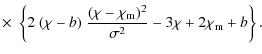
To derive expressions for the transformed signals, we assume that
precise redshift, or equivalently distance, information is available,
so that the survey can be sliced into thin tomographic bins. One can
then approximate
![]() ,
where
,
where ![]() is an appropriately chosen comoving distance in bin i. Here
is an appropriately chosen comoving distance in bin i. Here
![]() denotes the Dirac delta distribution. The lensing efficiency (2) can then be written in the form
denotes the Dirac delta distribution. The lensing efficiency (2) can then be written in the form
![\begin{displaymath}
g^{(j)}(\chi_i) \rightarrow g(\chi_j,\chi_i) \equiv \left\{ ...
...chi_i < \chi_j\\ [2mm]
0 &~~\mbox{else}.
\end{array} \right.
\end{displaymath}](/articles/aa/full_html/2010/09/aa14482-10/img41.png)
With these approximations the power spectra (1) and (3) turn into
where the dependence of the power spectra on the comoving distances of the two galaxy samples involved was made explicit. Note that if
2.2 Signal transformation
We seek to find linear combinations of tomographic second-order cosmic
shear measures such that in the resulting measures the cosmic shear
signal is largely suppressed with respect to the GI signal. The
starting point is analogous to the nulling technique as outlined by Joachimi & Schneider (2008). We define transformed power spectra as
where
Inserting (7) into the definition (8), one finds that
where we defined the function
Note that the integration absorbed into
Transforming the lensing signal analogously by plugging (6) into (8), one arrives at

Again, (10) was used to produce the final expression. The conditions
In reality line-of-sight information will not be available in terms of
comoving distances, but rather in terms of the observable redshift.
Furthermore the galaxy redshift distributions will have a finite width
and also overlap due to scatter, in particular if only photometric
redshift information is available as will be the case for the vast
majority of galaxies in future cosmic shear surveys. To arrive at a
practical prescription for constructing the transformed power spectra,
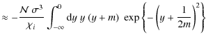
we therefore change the integration variable in (8) to redshift and subsequently discretise the integral, yielding
where
2.3 Solving for the weight function
In the foregoing section we saw that the GI signal can be boosted, and
the GG signal at the same time suppressed, by formulating conditions on
the function
![]() .
Via its defining equation (10) it is related to the weight function
.
Via its defining equation (10) it is related to the weight function
![]() that enters the transformation (8). Hence, to obtain a boosting transformation, one has to solve (10) for
that enters the transformation (8). Hence, to obtain a boosting transformation, one has to solve (10) for
![]() for a given function
for a given function
![]() .
.
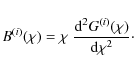
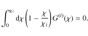
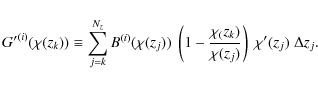
We begin by noting that (10)
is a Volterra integral equation of the first kind. It has a kernel that
is linear in the integration variable, so that one can readily solve
for the weight function by differentiating twice, resulting in
We have found the solution of the inhomogeneous Volterra equation (10) under the premises that
To find the solution of the homogeneous equation, obtained from (10) by setting
![]() ,
we define
,
we define
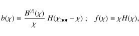
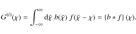
where
|
(15) |
The introduction of the Heaviside functions in (14) was used to extend the integration to zero and infinity. If we denote Fourier transforms by a tilde, the convolution theorem yields
Note the analogy between (10) and the definition of the lensing efficiency (2). This can be interpreted as
![]() being a modified lensing efficiency, which is then used to construct an
alternative lensing convergence with desired properties chosen via
being a modified lensing efficiency, which is then used to construct an
alternative lensing convergence with desired properties chosen via
![]() .
For details on this view see the motivation of the nulling technique given in Joachimi & Schneider (2008).
.
For details on this view see the motivation of the nulling technique given in Joachimi & Schneider (2008).
3 Construction of weights
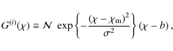
Apart from the requirements formulated in Sect. 2.2 to ensure a boosting of the GI signal with respect to cosmic shear, the choice of
![]() is arbitrary. In the following we choose a specific parametrisation of
is arbitrary. In the following we choose a specific parametrisation of
![]() which is convenient and intuitive, but not necessarily optimal. Its base is a Gaussian that is peaked at
which is convenient and intuitive, but not necessarily optimal. Its base is a Gaussian that is peaked at ![]() ,
which fosters a strong contribution of GI correlations via the first term of (9). Some additional flexibility is needed at
,
which fosters a strong contribution of GI correlations via the first term of (9). Some additional flexibility is needed at
![]() ,
allowing for sign changes of
,
allowing for sign changes of
![]() to downweight the lensing signal. We define
to downweight the lensing signal. We define
where
From this result and by means of (13) one readily obtains the weight function
| |
= | 
|
(18) |
|
The normalisation of
Note that since
Two of the remaining three free parameters of (16) will now be used to boost (9) and suppress (11). First, we demand that (16) is peaked at ![]() ,
i.e.
,
i.e.
![]() .
Using (17), we obtain
.
Using (17), we obtain
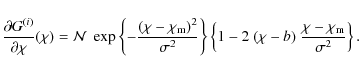
The second condition should render the integral in (11) close to zero. While it is possible to numerically determine for instance the parameter b such that this condition is fulfilled for every angular frequency individually, we prefer to proceed in a way that does not rely on a model of cosmic shear power spectra at all. We note that if the width of the Gaussian
Inserting (16) together with (20), and making the further definitions
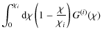
![$\displaystyle = - \frac{{\cal N}~ \sigma^3}{8 m^2 \chi_i} \left\{ 2m~ (1-2m^2) ...
... } + \sqrt{\pi} \left[ 1+{\rm Erf}\left( \frac{1}{2m} \right) \right] \right\}.$](/articles/aa/full_html/2010/09/aa14482-10/img102.png)
The approximation in the first equality refers to replacing the lower boundary of the integral
We have solved (21) directly and plot the resulting b in Fig. 1. We find excellent agreement with the approximate solution (23) as long as the assumption discussed above is fulfilled. Significant deviations from the linear behaviour of b as a function of
![\begin{figure}
\par\includegraphics[scale=0.365,angle=270,clip]{14482fg1.ps}
\end{figure}](/articles/aa/full_html/2010/09/aa14482-10/img112.png)
|
Figure 1:
Parameter b as a function of |
| Open with DEXTER | |
![\begin{figure}
\par\includegraphics[scale=.36,angle=270,clip]{14482fg2.ps}
\end{figure}](/articles/aa/full_html/2010/09/aa14482-10/img113.png)
|
Figure 2:
Functions
|
| Open with DEXTER | |
The conditions specified above are strictly fulfilled only for continuous ![]() or z. However, we will in practice use the discretised transformation (12)
and thus have to make sure that GI boosting and GG suppression work
accurately also in this case. Via a procedure outlined in the
following, we optimise the remaining free parameter
or z. However, we will in practice use the discretised transformation (12)
and thus have to make sure that GI boosting and GG suppression work
accurately also in this case. Via a procedure outlined in the
following, we optimise the remaining free parameter ![]() to guarantee a good sampling of
to guarantee a good sampling of
![]() by the discrete set of weights
by the discrete set of weights
![]() with
j=1, .. ,Nz, thereby fulfilling
with
j=1, .. ,Nz, thereby fulfilling
![]() and (21) to good accuracy.
and (21) to good accuracy.
As the sampling points of (12)
we choose the medians of the redshift distributions of the galaxy
samples employed. It is expected that the optimal choice of the
parameter ![]() ,
denoted by
,
denoted by
![]() in the following, will depend intricately on the positions of these
sampling points and hence on the redshift distributions of the
different galaxy samples in the cosmic shear data, in particular if the
number of sampling points is small, e.g. if the distributions have a
large scatter. Since the binning is done in terms of redshift, it is
convenient to work with the quantity
in the following, will depend intricately on the positions of these
sampling points and hence on the redshift distributions of the
different galaxy samples in the cosmic shear data, in particular if the
number of sampling points is small, e.g. if the distributions have a
large scatter. Since the binning is done in terms of redshift, it is
convenient to work with the quantity
![]() instead of
instead of ![]() .
We will also give our choices of
.
We will also give our choices of
![]() in terms of
in terms of ![]() throughout.
throughout.
We introduce the discrete version of the function
![]() ,
,
Then we consider the root mean square deviation of all function values
as a criterion for how well
In Fig. 2 we have plotted a selection of typical results for
![]() and the corresponding weight function
and the corresponding weight function
![]() .
As common features of
.
As common features of
![]() a distinct peak at zi and a negative dip at z<zi, the latter necessary to fulfil (21), are discernible. The weight function
a distinct peak at zi and a negative dip at z<zi, the latter necessary to fulfil (21), are discernible. The weight function
![]() has three pronounced extrema of which the central one is located at zi, plus a shallow fourth one at low redshift.
has three pronounced extrema of which the central one is located at zi, plus a shallow fourth one at low redshift.
Note that the method laid out here is completely independent of any
assumptions about the angular dependence of both the underlying lensing
and intrinsic alignment signals. To determine the weights
entering (12),
we only make use of the well-known redshift dependence of the GI and GG
signals, plus the redshift binning of the survey to be analysed. We
note that the weights
![]() depend on
depend on
![]() and possibly further cosmological parameters via the distance-redshift
relation. However, the same applies to the weights used in the standard
nulling technique, and from the investigation by Joachimi & Schneider (2009)
we conclude that this dependence is weak and that the assumption of an
incorrect cosmology when constructing the weights is uncritical.
and possibly further cosmological parameters via the distance-redshift
relation. However, the same applies to the weights used in the standard
nulling technique, and from the investigation by Joachimi & Schneider (2009)
we conclude that this dependence is weak and that the assumption of an
incorrect cosmology when constructing the weights is uncritical.
4 Modelling
To assess the performance of the boosting technique, we need to
model both the cosmic shear and the intrinsic alignment signals. To
this end, we assume a spatially flat ![]() CDM universe with matter density parameter
CDM universe with matter density parameter
![]() and Hubble parameter h=0.7. The matter power spectrum has a primordial slope
and Hubble parameter h=0.7. The matter power spectrum has a primordial slope
![]() and normalisation
and normalisation
![]() .
The transfer function is computed according to Eisenstein & Hu (1998), using a baryon density parameter of
.
The transfer function is computed according to Eisenstein & Hu (1998), using a baryon density parameter of
![]() ,
while the non-linear evolution of the power spectrum is determined by the fit formula of Smith et al. (2003).
,
while the non-linear evolution of the power spectrum is determined by the fit formula of Smith et al. (2003).
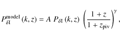
We use the linear alignment model (Hirata & Seljak 2004; Catelan et al. 2001) to calculate the matter density-intrinsic power spectrum,
where the normalisation is chosen such that
A cosmic shear survey is modelled by assuming an overall galaxy redshift distribution according to Smail et al. (1994),
with z0=0.64 and
We consider three different survey models which are summarised in Table 1. All of these surveys are assumed to cover the whole extragalactic sky, i.e.
![]() .
To calculate shape noise, we use an intrinsic ellipticity dispersion of
.
To calculate shape noise, we use an intrinsic ellipticity dispersion of
![]() throughout.
throughout.
First, we construct a ``spectroscopic'' survey S for which redshift bins are assigned with width 0.01(1+z)
and no scatter. In this case the signals are calculated to excellent
approximation not over the complete bin width, but at the median
redshifts of each bin. Whilst it is in principle possible to achieve
such a dense redshift binning and small scatter with photometric
redshifts (see e.g. Ilbert et al. 2009),
it is more likely that future large-area spectroscopic surveys fit into
this category. In any case the number of available galaxies will be
small. Taking the wide spectroscopic survey of the Euclid mission as
reference (Laureijs et al. 2009), we set the overall galaxy number density to
![]() .
.
Table 1: Overview on the different survey models used.
Second, we create a survey that features high-quality photometric
redshift data, termed P1. We choose the same binning scheme as for the
first case, but introduce a photometric redshift scatter of
![]() ,
corresponding to the target value of the Euclid imaging survey. To be
conservative, we assume that this photometric redshift quality is only
attainable for a subset of galaxies and set
,
corresponding to the target value of the Euclid imaging survey. To be
conservative, we assume that this photometric redshift quality is only
attainable for a subset of galaxies and set
![]() .
Finally, we make use of a setup P2 with redshift binning in steps of 0.02(1+z) and scatter
.
Finally, we make use of a setup P2 with redshift binning in steps of 0.02(1+z) and scatter
![]() ,
which can be regarded as representative of a standard future imaging survey designed to do cosmic shear. Again referring to Laureijs et al. (2009), we adopt
,
which can be regarded as representative of a standard future imaging survey designed to do cosmic shear. Again referring to Laureijs et al. (2009), we adopt
![]() in this case.
in this case.
The photometric redshift bin widths are chosen such that the associated
distributions of neighbouring bins can still be well distinguished. We
have found that narrowing the bin widths substantially below about
![]() deteriorates the performance of the boosting technique. It should be
noted that spectroscopic redshifts as well as photometric redshifts of
high quality are usually limited to a brighter subset of galaxies,
therefore altering the overall redshift distribution of galaxies.
However, to facilitate the comparison between the three survey models
under scrutiny, we keep
deteriorates the performance of the boosting technique. It should be
noted that spectroscopic redshifts as well as photometric redshifts of
high quality are usually limited to a brighter subset of galaxies,
therefore altering the overall redshift distribution of galaxies.
However, to facilitate the comparison between the three survey models
under scrutiny, we keep
![]() as specified above.
as specified above.
With the three-dimensional GG and GI power spectra and the redshift distributions
![]() at hand, one can calculate the tomographic power spectra according to (1) and (3). For the further analysis we divide the angular frequency range into
at hand, one can calculate the tomographic power spectra according to (1) and (3). For the further analysis we divide the angular frequency range into
![]() logarithmic bins between
logarithmic bins between ![]() and
and
![]() .
.
5 Performance of GI boosting
5.1 Boosted signals
![\begin{figure}
\par\includegraphics[scale=.35,angle=270,clip]{14482fg3.ps}\vspace*{-1.5mm}
\end{figure}](/articles/aa/full_html/2010/09/aa14482-10/img147.png)
|
Figure 3:
Diagnostic |
| Open with DEXTER | |
To condense the performance of the boosting technique into a single
number, we define the median with respect to angular frequency of the
ratio of GI over GG signal,
where X can be replaced by any tomography power spectrum
In Fig. 3 we show
![]() ,
together with the diagnostic
,
together with the diagnostic ![]() as defined in (25), as a function of
as defined in (25), as a function of ![]() for one zi per survey model. Overall we find that small values of
for one zi per survey model. Overall we find that small values of ![]() indeed indicate regimes of
indeed indicate regimes of ![]() in which the GI signal is well boosted. It is important to note that the absolute value of
in which the GI signal is well boosted. It is important to note that the absolute value of ![]() is meaningless due to the arbitrariness in the overall amplitude of
is meaningless due to the arbitrariness in the overall amplitude of
![]() .
When
.
When
![]() is no longer well sampled for small
is no longer well sampled for small ![]() ,
,
![]() features a clear increase. Sometimes secondary minima in
features a clear increase. Sometimes secondary minima in ![]() can be observed, see the centre panel of Fig. 3, which is caused by the sampling points being consecutively placed at the extrema of
can be observed, see the centre panel of Fig. 3, which is caused by the sampling points being consecutively placed at the extrema of
![]() .
Thereby, although only sparsely sampled, the discrete form (24) captures the main characteristics of
.
Thereby, although only sparsely sampled, the discrete form (24) captures the main characteristics of
![]() and hence can well represent
and hence can well represent
![]() ,
yielding a small value of
,
yielding a small value of ![]() .
.
Table 2:
Summary of
![]() for different values of zi and the three survey models.
for different values of zi and the three survey models.
In the top panel of Fig. 3
![]() for both surveys S and P1 is given. Since the binning scheme is identical for both surveys,
for both surveys S and P1 is given. Since the binning scheme is identical for both surveys, ![]() is the same. This example demonstrates that
is the same. This example demonstrates that
![]() depends considerably on the details of the actual signals, in this case a change from
depends considerably on the details of the actual signals, in this case a change from
![]() to
to
![]() .
The diagnostic
.
The diagnostic ![]() does not trace the boosting of the actual signals and can consequently not be exploited to find the maximum
does not trace the boosting of the actual signals and can consequently not be exploited to find the maximum
![]() .
However, for both surveys
.
However, for both surveys ![]() identifies the regime of small
identifies the regime of small ![]() in which the boosting performs worse and which thus should be avoided. In the case
in which the boosting performs worse and which thus should be avoided. In the case
![]() the sampling in redshift becomes fully insufficient for small
the sampling in redshift becomes fully insufficient for small ![]() .
Accordingly,
.
Accordingly, ![]() rises sharply, and the GG signal starts to dominate again.
rises sharply, and the GG signal starts to dominate again.
The optimal width of
![]() can be chosen freely in the interval where
can be chosen freely in the interval where ![]() is stable and small. If there is a clear minimum, we place
is stable and small. If there is a clear minimum, we place
![]() there; otherwise we set
there; otherwise we set
![]() to a small value in the interval where
to a small value in the interval where ![]() is small, see e.g. the centre panel of Fig. 3. This assignment of
is small, see e.g. the centre panel of Fig. 3. This assignment of
![]() may not be unique, but it is uncritical. Note that the weight functions
corresponding to the optimum cases of the examples shown in Fig. 3 are those depicted in Fig. 2. We emphasise again that
may not be unique, but it is uncritical. Note that the weight functions
corresponding to the optimum cases of the examples shown in Fig. 3 are those depicted in Fig. 2. We emphasise again that
![]() cannot be measured from real data, and accordingly we do not use this quantity to determine
cannot be measured from real data, and accordingly we do not use this quantity to determine
![]() .
.
One might expect that the denser the sampling points of
![]() and
and
![]() can be placed, the more sharply peaked weight functions can be well
represented by the discrete sampling, and thus smaller values of
can be placed, the more sharply peaked weight functions can be well
represented by the discrete sampling, and thus smaller values of ![]() could be chosen. However, consider the case
could be chosen. However, consider the case
![]() and zi=0.98 which is shown in the bottom panels of both Figs. 2 and 3. Although
and zi=0.98 which is shown in the bottom panels of both Figs. 2 and 3. Although
![]() is small compared to e.g. our findings for survey P1, the sparse
sampling obviously captures the main features of the weight function
and hence results in a small
is small compared to e.g. our findings for survey P1, the sparse
sampling obviously captures the main features of the weight function
and hence results in a small ![]() .
.
![\begin{figure}
\par\includegraphics[scale=.35,angle=270,clip]{14482fg4.ps}\vspace*{1.2mm}
\end{figure}](/articles/aa/full_html/2010/09/aa14482-10/img153.png)
|
Figure 4:
Left column: Example set of lensing (GG) and intrinsic alignment (GI) tomography power spectra for the spectroscopic survey S and zi=0.53.
The GG signal is shown as solid line, the GI signal as dotted line. The
upper three panels show power spectra for different background bins j, i.e. auto-correlations (j=i, ``auto''), cross-correlations with a bin at intermediate redshift (
j=(i+Nz)/2, ``mid''), and cross-correlations with the most distant bin (j=Nz,
``far''). In the bottom panel the transformed GG and GI signals are
plotted (``boost''). Note that absolute values of the power spectra are
shown throughout. Centre column: Same as above, but for the survey P1 (
|
| Open with DEXTER | |
In Fig. 4 we have plotted example sets of original and transformed power spectra, the latter each computed for the optimal values of ![]() .
Table 2 lists the corresponding values of
.
Table 2 lists the corresponding values of
![]() and
and
![]() for the three survey models and three redshifts zi each, including the cases depicted in the figure. The GI over GG ratio
for the three survey models and three redshifts zi each, including the cases depicted in the figure. The GI over GG ratio
![]() for the original power spectra ranges from about
for the original power spectra ranges from about ![]() to
to ![]() .
For a correlation between galaxy samples i and j with zi < zj,
.
For a correlation between galaxy samples i and j with zi < zj,
![]() increases strongly with the separation between zj and zi. Both the GI and GG signals show this behaviour due to (2). Since the cosmic shear signal is generated by all the matter between z=0 and zi with the highest efficiency at zi/2, whereas the intrinsic alignment contribution stems form matter around zi, the GI signal has the stronger dependence on redshift, causing the increase in
increases strongly with the separation between zj and zi. Both the GI and GG signals show this behaviour due to (2). Since the cosmic shear signal is generated by all the matter between z=0 and zi with the highest efficiency at zi/2, whereas the intrinsic alignment contribution stems form matter around zi, the GI signal has the stronger dependence on redshift, causing the increase in
![]() .
For the non-linear version of the linear alignment model this effect
can lead to a GI signal whose absolute value can come close to or even
surpass the cosmic shear signal for large zj-zi, see e.g. also Bridle & King (2007).
.
For the non-linear version of the linear alignment model this effect
can lead to a GI signal whose absolute value can come close to or even
surpass the cosmic shear signal for large zj-zi, see e.g. also Bridle & King (2007).
It is evident from Table 2
that the better resolved the redshift information is, the more can the
GI signal be boosted. For quasi-spectroscopic data, the residual GG
contribution is well below the ![]() -level and hence expected to be negligible. In the case zi=0.76 we find by chance a near-total cancellation of the cosmic shear signal. For good photo-z data with
-level and hence expected to be negligible. In the case zi=0.76 we find by chance a near-total cancellation of the cosmic shear signal. For good photo-z data with
![]() the method is also effective, yielding
the method is also effective, yielding
![]() well in excess of 10, so that any biases due to the residual GG
contribution are likely to remain below the statistical errors of
intrinsic alignment parameters. For survey P2 it is still possible to
produce a dominating GI signal, with
well in excess of 10, so that any biases due to the residual GG
contribution are likely to remain below the statistical errors of
intrinsic alignment parameters. For survey P2 it is still possible to
produce a dominating GI signal, with
![]() between approximately 6 and 12, but a GG residual exceeding
between approximately 6 and 12, but a GG residual exceeding ![]() may require further treatment to avoid a significant bias.
may require further treatment to avoid a significant bias.
5.2 Parameter constraints
The boosted GI signal has the potential use of directly constraining
models of intrinsic alignments, provided that the statistical power is
sufficiently high and that systematics due to residual GG contributions
are under control. We set up a simple intrinsic alignment model and use
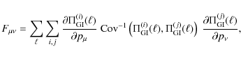
the Fisher matrix formalism (Tegmark et al. 1997) to forecast expected errors and biases on its free parameters. We define
where
Assuming that the signal covariance is itself not parameter-dependent,
which holds to very good accuracy for the large survey we consider (Eifler et al. 2009), the Fisher matrix reads
for a parameter vector
| |
= | 
|
(31) |
The power spectrum covariance in turn is given by (see Joachimi et al. 2008, and references therein)
where
The bias formalism (e.g. Huterer et al. 2006; Joachimi & Schneider 2009; Amara & Réfrégier 2008)
allows us to compute the bias on the intrinsic alignment parameters due
to the residual GG signal in the transformed power spectra via
Note that, contrary to works focusing on cosmic shear analyses and treating intrinsic alignments as the systematic, we use the GI contribution in (30) and insert the transformed GG signal into (33) such that it plays the role of a systematic. We make the assumption that, given zi<zj, the galaxy redshift distribution p(i)(z) entering (3) is sufficiently compact that we can take the term
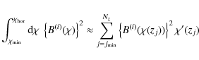
Since at this point we merely seek to demonstrate the concept of boosting, we limit the set of
![]() entering (30) to those bins i which fulfil
entering (30) to those bins i which fulfil
![]() .
This ensures that the approximation (22) can be used throughout and that it is straightforward to assign
.
This ensures that the approximation (22) can be used throughout and that it is straightforward to assign
![]() .
Besides, we avoid issues at high zi with non-zero
.
Besides, we avoid issues at high zi with non-zero
![]() ,
which could possibly violate the basic condition
,
which could possibly violate the basic condition
![]() ,
see Sect. 2.3. We determine
,
see Sect. 2.3. We determine
![]() by computing the diagnostic
by computing the diagnostic ![]() given by (25) for all zi and devising simple, piecewise linear formulae which yield a
given by (25) for all zi and devising simple, piecewise linear formulae which yield a
![]() in the regime of small
in the regime of small ![]() for every zi. For survey P2 (standard photo-z) we use
for every zi. For survey P2 (standard photo-z) we use
![]() .
The two other surveys have the same redshift binning and hence identical
.
The two other surveys have the same redshift binning and hence identical ![]() .
We set
.
We set
![]() for
for
![]() and
and
![]() for zi > 1 in these cases.
for zi > 1 in these cases.
Table 3:
Statistical errors
![]() and residual biases
and residual biases
![]() for the different survey models used.
for the different survey models used.
Now we are in the position to compute the boosting transformation for power spectra with
![]() .
By means of (30) and (33)
we obtain statistical and systematic error estimates for both intrinsic
alignment parameters for all three survey models, summarised in
Table 3. When varying both parameters, we find marginalised
.
By means of (30) and (33)
we obtain statistical and systematic error estimates for both intrinsic
alignment parameters for all three survey models, summarised in
Table 3. When varying both parameters, we find marginalised ![]() errors of approximately 2.9 for A and 7.4 for
errors of approximately 2.9 for A and 7.4 for ![]() in case of survey S. The two surveys with photometric redshift data produce errors around 0.7 on A and of the order 2 for
in case of survey S. The two surveys with photometric redshift data produce errors around 0.7 on A and of the order 2 for ![]() .
As expected, the bias due to the remaining cosmic shear signal is
negligible in the case of the spectroscopic survey S and clearly
subdominant in the case of survey P1. Even for the standard photo-z
setup P2 biases remain within the statistical
.
As expected, the bias due to the remaining cosmic shear signal is
negligible in the case of the spectroscopic survey S and clearly
subdominant in the case of survey P1. Even for the standard photo-z
setup P2 biases remain within the statistical ![]() errors, reaching up to
errors, reaching up to
![]() for A.
for A.
In Fig. 5 the corresponding ![]() confidence contours in the parameter plane
confidence contours in the parameter plane
![]() are given for the three survey models. As we have chosen a pivot
redshift which is below the minimum redshift of GI signals that enter
the analysis, a positive
are given for the three survey models. As we have chosen a pivot
redshift which is below the minimum redshift of GI signals that enter
the analysis, a positive ![]() leads to an increase in the amplitude of the GI model, which can be compensated by a smaller A. Hence, A and
leads to an increase in the amplitude of the GI model, which can be compensated by a smaller A. Hence, A and ![]() are anti-correlated, leading to the degeneracy as indicated by the error ellipses. The bias acts mainly on A because a residual GG signal will to zeroth order affect the overall amplitude of the signal. In all three cases the
are anti-correlated, leading to the degeneracy as indicated by the error ellipses. The bias acts mainly on A because a residual GG signal will to zeroth order affect the overall amplitude of the signal. In all three cases the ![]() contours comfortably enclose the fiducial, true parameter values.
contours comfortably enclose the fiducial, true parameter values.
Due to the low number density of galaxies, survey S is clearly not competitive in constraints on intrinsic alignment properties. The results from the two other surveys are not capable of pinning down the intrinsic alignment model with high precision, but their bounds are comparable to current constraints by analyses of spectroscopic measurements of galaxy number density-shape cross-correlations (Mandelbaum et al. 2009). Note that the weights used for this analysis may still have considerable room for optimisation, and that we only used a limited range of zi.
![\begin{figure}
\par\includegraphics[scale=.6,clip]{14482fg5.ps}
\end{figure}](/articles/aa/full_html/2010/09/aa14482-10/img180.png)
|
Figure 5:
Constraints on the free parameters of the GI model. Shown are the |
| Open with DEXTER | |
Table 3 also lists the resulting errors when only A
is varied and no additional redshift dependence of the intrinsic
alignment model is assumed. Constraints improve significantly when
lifting the degeneracy with ![]() such that A is determined to better than
such that A is determined to better than
![]() for the survey models with photometric redshifts while constraints by
survey S are about three times weaker. The bias is still negligible for
the spectroscopic survey model, and clearly subdominant for survey P1 (
for the survey models with photometric redshifts while constraints by
survey S are about three times weaker. The bias is still negligible for
the spectroscopic survey model, and clearly subdominant for survey P1 (
![]() ). The residual systematic affects the error budget noticeably for the analysis of survey P2 (
). The residual systematic affects the error budget noticeably for the analysis of survey P2 (
![]() )
with
)
with
![]() .
Again, optimisation of the boosting procedure may further decrease the residual cosmic shear signal well below the statistical
.
Again, optimisation of the boosting procedure may further decrease the residual cosmic shear signal well below the statistical ![]() -limit.
-limit.
The errors for the good photo-z and in particular the spectroscopic survey models are dominated by shape noise due to the low number density of galaxies in each tomographic galaxy sample, apart from only the smallest angular frequencies. As can be seen from (32), the errors scale inversely with the total number of galaxies in the survey if cosmic variance is negligible. Thus, if in the future larger number densities of galaxies with highly accurate photometric redshifts than assumed in this work are attainable, the constraints on GI correlations via the boosting technique will improve accordingly. If we re-run the analysis for survey S with the galaxy number density assumed for survey P1, i.e. a factor of 10 higher, all the statistical errors indeed decrease by almost an order of magnitude.
6 Relation to GI nulling
If one is able to extract the GI signal from cosmic shear data, the question arises whether this could also be used to remove the GI contamination from the data and thus make cosmic shear analyses robust against biases due to intrinsic alignments. Intuitively, one can simply subtract an isolated GI signal from the original measures, and indeed we are going to devise such a procedure. Afterwards we will again propose a simple, parametric weight function to construct a boosting method, whose outcome will then be used to eliminate the GI signal. These steps are not optimised and merely serve to demonstrate the link between GI boosting and its removal, as well as to compare the performance of the latter to the standard nulling technique of Joachimi & Schneider (2009,2008) in a simple scenario.
6.1 Signal transformation
As an alternative to the procedure in Sect. 2.2, one can choose the lower integration boundary in (8) as
![]() .
As is evident from (9), in this case only the first term of the transformed GI signal remains. Hence, it is likely that
.
As is evident from (9), in this case only the first term of the transformed GI signal remains. Hence, it is likely that
![]() produces a larger amplitude of the modified GI power spectrum, but
produces a larger amplitude of the modified GI power spectrum, but
![]() results in a cleaner signal insofar as it contains only contributions from intrinsic alignments generated by matter at distance
results in a cleaner signal insofar as it contains only contributions from intrinsic alignments generated by matter at distance ![]() .
Consequently, we are going to use the latter choice of
.
Consequently, we are going to use the latter choice of
![]() for constructing a method to remove the GI signal at
for constructing a method to remove the GI signal at ![]() .
The transformed lensing signal for
.
The transformed lensing signal for
![]() is derived in analogy to (11) and reads
is derived in analogy to (11) and reads
Now suppose we are able to construct a boosting technique with a significant signal
and likewise for the individual GG and GI signals. This definition holds for all i < j. The auto-correlations
Assuming that the GI boosting works effectively,
![]() ,
so that one expects that
,
so that one expects that
![]() ,
i.e. the transformed cosmic shear signal is close to the original GG
term. Switching to the notation of narrow redshift bins again, we find
for the transformed GI signal
,
i.e. the transformed cosmic shear signal is close to the original GG
term. Switching to the notation of narrow redshift bins again, we find
for the transformed GI signal
| |
= | 
|
(36) |
|
where we have inserted (7) and the first term of (9), and made use of the transition
Note that the standard nulling technique as presented in Joachimi & Schneider (2008) also makes use of the definition (8) with
![]() .
The central condition in their approach is recovered in our formalism by requiring
.
The central condition in their approach is recovered in our formalism by requiring
![]() ,
which eliminates the GI signal under the same assumption of narrow redshift bins, see (9). For practical purposes we also switch to the discretised form of the signal transformation (12), using now
,
which eliminates the GI signal under the same assumption of narrow redshift bins, see (9). For practical purposes we also switch to the discretised form of the signal transformation (12), using now
![]() .
.
6.2 Construction of weights
We begin by developing again a boosting technique, now for the changed condition
![]() .
Due to the associated change in the lower boundary of integration in (8), the condition to remove the GG signal is altered as well. Keeping the same approximations as used to derive (21), we now obtain from (34)
.
Due to the associated change in the lower boundary of integration in (8), the condition to remove the GG signal is altered as well. Keeping the same approximations as used to derive (21), we now obtain from (34)
where we executed the integration over
Inserting (13) into the foregoing definition and integrating by parts, one arrives at the useful relations
| |
= | 
|
(39) |
| = | 
|
When these are plugged into (37), we obtain a condition which is the equivalent of (21), i.e. which ensures the suppression of the GG signal in the transformed power spectra (8),
In contrast to (21), which is an integral condition on
| |
(41) | ||
|
where the integrals (38) were transformed to redshift and discretised in analogy to (12).
Moreover, (40) hinders us to impose the condition
![]() again, which boosted the GI term, see (9). We define
again, which boosted the GI term, see (9). We define
which has one free parameter less than (16). To avoid any confusion with foregoing usage, we will add a sub- or superscript Q to indicate quantities which are used in this section for devising a nulling procedure. The condition (40) readily implies

|
(43) |
Therefore
The normalisation
6.3 Nulled signals
![\begin{figure}
\par\includegraphics[scale=.37,angle=270,clip]{14482fg6.ps}
\vspace*{2.5mm}\end{figure}](/articles/aa/full_html/2010/09/aa14482-10/img220.png)
|
Figure 6:
Determination of
|
| Open with DEXTER | |
Table 4: Summary of the nulling performance for two survey models and different values of zi.
Again we study a set of diagnostics as a function of ![]() to identify regimes of
to identify regimes of ![]() where the GI nulling performs well. In Fig. 6 we plot
where the GI nulling performs well. In Fig. 6 we plot ![]() as defined in (25),
as defined in (25), ![]() which assesses how (40) is affected by the discretisation, and
which assesses how (40) is affected by the discretisation, and
![]() as an indicator of the boosting of the GI signal in the
as an indicator of the boosting of the GI signal in the
![]()
![]() , for the spectroscopic survey S at zi=0.53. Furthermore we show the GI over GG ratio
, for the spectroscopic survey S at zi=0.53. Furthermore we show the GI over GG ratio
![]() ,
which is given by (28) when replacing X by the nulled power spectra (35). Note that small values of
,
which is given by (28) when replacing X by the nulled power spectra (35). Note that small values of
![]() are indicative of an effective removal of the GI signal.
are indicative of an effective removal of the GI signal.
One might expect that [0pt]
![]() is largest for small
is largest for small ![]() because [0pt]
because [0pt]
![]() is
sharply peaked with a large maximum value. However, this effect is
counteracted by the normalisation of the weight function. Large values
of
is
sharply peaked with a large maximum value. However, this effect is
counteracted by the normalisation of the weight function. Large values
of ![]() cause [0pt]
cause [0pt]
![]() to be smoother, i.e. to have smaller curvature. Due to (13) the amplitude of [0pt]
to be smoother, i.e. to have smaller curvature. Due to (13) the amplitude of [0pt]
![]() would thus decrease for fixed normalisation. Since we normalise [0pt]
would thus decrease for fixed normalisation. Since we normalise [0pt]
![]() according to (19) for every
according to (19) for every ![]() individually, large
individually, large ![]() yield a higher normalisation relative to small
yield a higher normalisation relative to small ![]() ,
implying also larger values of [0pt]
,
implying also larger values of [0pt]
![]() .
Hence, one observes an increase in [0pt]
.
Hence, one observes an increase in [0pt]
![]() as a function of
as a function of ![]() .
.
![\begin{figure}
\par\includegraphics[scale=.42,angle=270,clip]{14482fg7.ps}
\end{figure}](/articles/aa/full_html/2010/09/aa14482-10/img245.png)
|
Figure 7:
Nulling performance for the spectroscopic survey S at zi=0.53. Top panel: Transformed GG (solid curve) and GI (dotted curve) power spectra, computed according to (8). Centre panel: GI over GG ratio
|
| Open with DEXTER | |
The diagnostic ![]() has relatively large values for strongly peaked [0pt]
has relatively large values for strongly peaked [0pt]
![]() and decreases slowly for larger
and decreases slowly for larger ![]() .
A small change in the weight function [0pt]
.
A small change in the weight function [0pt]
![]() due to the discretisation can induce significant changes in [0pt]
due to the discretisation can induce significant changes in [0pt]
![]() ,
and its slope close to
,
and its slope close to ![]() ,
which are the stronger the more sharply peaked [0pt]
,
which are the stronger the more sharply peaked [0pt]
![]() is. Therefore (40) is more difficult to fulfil at small
is. Therefore (40) is more difficult to fulfil at small ![]() .
Both [0pt]
.
Both [0pt]
![]() and
and ![]() prefer larger
prefer larger ![]() ,
in agreement with
,
in agreement with ![]() ,
which we thus continue to use for the determination of
,
which we thus continue to use for the determination of
![]() .
As
.
As ![]() clearly disfavours
clearly disfavours
![]() ,
we choose as the optimum the minimum of
,
we choose as the optimum the minimum of ![]() at about 0.28. Considering the lower panel of Fig. 6, this value is in very good agreement with small and hence close to optimal values of
at about 0.28. Considering the lower panel of Fig. 6, this value is in very good agreement with small and hence close to optimal values of
![]() .
Generally, we find that
.
Generally, we find that
![]() is considerably larger for this approach, compared to the variant analysed in Sect. 5.
is considerably larger for this approach, compared to the variant analysed in Sect. 5.
With this finding at hand, we can compute GI-boosted power spectra according to (8), and from these sets of nulled power spectra via (35), results for both being shown in Fig. 7. The GI term is significantly less boosted than in the version studied in Sect. 5.1 with
![]() less than 10 (see Table 2, for comparison). Still, the intrinsic alignment suppression works excellently with
less than 10 (see Table 2, for comparison). Still, the intrinsic alignment suppression works excellently with
![]() for all background redshift bins and angular frequencies.
for all background redshift bins and angular frequencies.
In Table 4 values of
![]() for other zi
and in addition for the good photo-z survey P1 are listed. The
downweighting of the GI signal quickly deteriorates with the increase
in photometric redshift uncertainty, being more than two orders of
magnitude larger for survey P1. For the standard photo-z case we find
that the boosting as implemented in this section is ineffective, so
that we do not consider it here. As shown in Sect. 6.1, under idealistic circumstances one expects the signal in the nulled power spectra
for other zi
and in addition for the good photo-z survey P1 are listed. The
downweighting of the GI signal quickly deteriorates with the increase
in photometric redshift uncertainty, being more than two orders of
magnitude larger for survey P1. For the standard photo-z case we find
that the boosting as implemented in this section is ineffective, so
that we do not consider it here. As shown in Sect. 6.1, under idealistic circumstances one expects the signal in the nulled power spectra
![]() to be close to the one in the original power spectra
to be close to the one in the original power spectra
![]() .
Hence, we calculate the quantity
.
Hence, we calculate the quantity
|
(45) |
which is also given in Fig. 7 and Table 4. The deviation from the original signal is at the per cent level for close foreground and background redshift bins with
6.4 Information content
How does the nulling technique as outlined above perform in comparison with the standard nulling approach? For a very dense binning in redshift both methods evidently remove the GI contamination of the cosmic shear signal to high accuracy, see for instance the recent findings by Shi et al. (2010). However, Joachimi & Schneider (2009) have shown that, even in idealistic situations comparable to our spectroscopic survey, a substantial loss of cosmological information is inherent to standard nulling. We assess the information content in both nulling approaches in a simple case study.
We restrict ourselves to the spectroscopic survey model S and consider again only
![]() ,
for the same reasons as discussed in Sect. 5.2. Again, we compute
,
for the same reasons as discussed in Sect. 5.2. Again, we compute ![]() for all zi to find a simple prescription for
for all zi to find a simple prescription for
![]() ;
in this case we use
;
in this case we use
![]() .
The information content is quantified in terms of the cumulative signal-to-noise (S/N), defined as
.
The information content is quantified in terms of the cumulative signal-to-noise (S/N), defined as
where the covariance of the nulled power spectra can be derived from (35),
| |
= | (47) | |
The S/N for data sets of original power spectra
Note that for every zi one can make use of Nz-i power spectra
![]() .
The very same number of modes is available in the standard nulling
approach although one mode is discarded to perform the actual nulling
(for details see Joachimi & Schneider 2009). Transformed auto-correlation power spectra with i=j do not enter the S/N, but by construction the
.
The very same number of modes is available in the standard nulling
approach although one mode is discarded to perform the actual nulling
(for details see Joachimi & Schneider 2009). Transformed auto-correlation power spectra with i=j do not enter the S/N, but by construction the
![]() do contribute to all
do contribute to all
![]() via the
via the
![]() ,
whereas in standard nulling auto-correlations are completely discarded.
However, due to the dense redshift binning, we expect the amount of
independent information contained in auto-correlation power spectra to
be small.
,
whereas in standard nulling auto-correlations are completely discarded.
However, due to the dense redshift binning, we expect the amount of
independent information contained in auto-correlation power spectra to
be small.
Table 5: Ratio of cumulative signal-to-noise of the nulled set of power spectra over the original set of power spectra (SNR).
We have given the resulting ratios of the S/N for the nulled data set over the S/N for the original one in Table 5. The considerable loss of information can be confirmed, the S/N for both nulling methods yielding less than ![]() of the original S/N. We find that these numbers are very robust against changes in the number and values of redshift bins i included in the S/N by varying the size of steps in bin numbers i
and the range of redshifts considered. It is quite remarkable that the
ratios for both nulling methods are very similar. The slightly bigger
number for the nulling as devised in this work could be related to the
inclusion of auto-correlation power spectra, but is not very
significant anyway.
of the original S/N. We find that these numbers are very robust against changes in the number and values of redshift bins i included in the S/N by varying the size of steps in bin numbers i
and the range of redshifts considered. It is quite remarkable that the
ratios for both nulling methods are very similar. The slightly bigger
number for the nulling as devised in this work could be related to the
inclusion of auto-correlation power spectra, but is not very
significant anyway.
In the standard nulling case the information loss is caused by discarding part of the signal, namely one mode per bin i whereas the variant suggested here features a signal that deviates by at most about ![]() from the untransformed one. In the latter case the loss is caused by an
increase in the covariance due to the subtraction of signals in (35).
We conjecture at this point that the agreement in the amount of
information lost, in spite of the largely different mechanisms of the
two methods, hints at a fundamental limit of how far GI and GG signals
can be distinguished by only relying on the redshift dependence of the
two contributions.
from the untransformed one. In the latter case the loss is caused by an
increase in the covariance due to the subtraction of signals in (35).
We conjecture at this point that the agreement in the amount of
information lost, in spite of the largely different mechanisms of the
two methods, hints at a fundamental limit of how far GI and GG signals
can be distinguished by only relying on the redshift dependence of the
two contributions.
7 Conclusions
In this paper we presented a method which extracts shear-ellipticity correlations (the GI signal) from a tomographic cosmic-shear data set. The approach relies neither on models of intrinsic alignments nor on knowledge of the cosmological parameters that characterise the cosmic shear (GG) signal, making only use of the typical and well-understood redshift dependencies of both the GI and GG term. We derived constraints which a linear transformation of second-order cosmic shear measures has to fulfil in order to boost the GI signal and simultaneously suppress the lensing contribution. We studied in depth a particular parametrisation of the weights entering this transformation and analysed the performance of the resulting GI boosting technique for three representative survey models.
Applying the GI boosting to future all-sky cosmic shear
surveys, it should be possible to isolate the GI signal with
subdominant biases due to a residual GG term, and with constraints that
are comparable to current results from indirect measurements of
shear-ellipticity correlations (Mandelbaum et al. 2009).
If one restricts the analysis to galaxies with photometric redshift
information of good quality, i.e. a redshift scatter of not more than
![]() with
with
![]() ,
one can achieve
,
one can achieve ![]() -errors on the GI signal amplitude A in the parametrisation of (29)
of better than 0.2 when varying only the amplitude, and a marginalised
error of approximately 0.7 when fitting an additional redshift
dependence.
-errors on the GI signal amplitude A in the parametrisation of (29)
of better than 0.2 when varying only the amplitude, and a marginalised
error of approximately 0.7 when fitting an additional redshift
dependence.
Using all galaxies from a survey fulfilling
![]() ,
the statistical constraints degrade only marginally but the parameter
bias due to the residual GG contribution can attain more significant
values of up to
,
the statistical constraints degrade only marginally but the parameter
bias due to the residual GG contribution can attain more significant
values of up to
![]() .
We also considered a survey with high-quality photometric or
spectroscopic redshifts. However, the expected low number density of
galaxies of
.
We also considered a survey with high-quality photometric or
spectroscopic redshifts. However, the expected low number density of
galaxies of
![]() ,
even for future surveys, does not permit us to place competitive
constraints on intrinsic alignment models. In this case of highly
accurate redshift information the residual bias on parameters is
negligible.
,
even for future surveys, does not permit us to place competitive
constraints on intrinsic alignment models. In this case of highly
accurate redshift information the residual bias on parameters is
negligible.
Although we have modelled scatter in photometric redshifts for our investigations, we did not consider other effects affecting the accuracy of redshift information, such as an error in the median of the galaxy redshift distributions or catastrophic failures in the determination of photometric redshifts. As several studies of intrinsic alignment removal techniques have demonstrated (e.g. Joachimi & Schneider 2009; Joachimi & Bridle 2009; Bridle & King 2007), the ability to separate the GI from the GG signal depends vitally on these parameters characterising the accuracy of and knowledge about redshifts. The same can be expected for the GI boosting technique, possibly to an even larger extent since in this case one attempts to suppress the originally strongest contribution to ellipticity correlations, the GG signal. Hence, we hypothesise that the requirements of future ambitious weak lensing surveys, like a negligible fraction of catastrophic failures and an error in the mean of each redshift distribution of not more than 0.002(1+ z) (Laureijs et al. 2009), are both necessary and sufficient for a success of GI boosting. We leave a detailed assessment of the requirements on the quality of redshift information to future work.
Moreover, we did not yet include intrinsic ellipticity
correlations (II) into our considerations. Since the II signal is
generated by physically close pairs of galaxies, it has a redshift
dependence that is clearly distinct from the GI and GG terms, and can
thus be removed relatively easily (King & Schneider 2002,2003; Heymans & Heavens 2003; Takada & White 2004).
In tomographic cosmic shear data it mainly affects auto-correlations
and cross-correlations of adjacent photometric redshift bins with
significant overlap of their corresponding distributions of true
redshifts. One of the aforementioned II removal techniques could
precede the GI boosting, causing an increased shape noise contribution
in particular in the auto-correlations due to the reduced number of
available galaxy pairs. Alternatively, the downweighting of the II
signal could also be readily incorporated into the boosting technique
by introducing the additional condition
![]() ,
implying
,
implying
![]() and therefore a downweighting of auto-correlations as well as cross-correlations of adjacent redshift distributions, see (8).
and therefore a downweighting of auto-correlations as well as cross-correlations of adjacent redshift distributions, see (8).
Our findings still have the potential for significant improvement
because we have only considered one specific parametrisation of the
weight function that governs the boosting transformation. While this
choice is intuitive and allows analytical progress, a more versatile
approach could be to assume the weight function
![]() as piecewise linear, with nodes placed at the median redshift of every
galaxy redshift sample. The constraints on GI boosting and GG
suppression could then be directly imposed on the discretised version
of the boosting transformation, thereby fixing a subset of the values
of
as piecewise linear, with nodes placed at the median redshift of every
galaxy redshift sample. The constraints on GI boosting and GG
suppression could then be directly imposed on the discretised version
of the boosting transformation, thereby fixing a subset of the values
of
![]() at its nodes. The remaining freedom in the weight function could for
instance be used to maximise the signal-to-noise of the expected
transformed GI signal.
at its nodes. The remaining freedom in the weight function could for
instance be used to maximise the signal-to-noise of the expected
transformed GI signal.
We also constructed a method of GI removal, directly based on a slightly modified version of the GI boosting technique. In principle, we showed that if one is able to isolate the GI signal via boosting, one can simply subtract a rescaled version of the GI term from the original cosmic shear measures to eliminate the intrinsic alignment systematic. We find that the residual contamination of the cosmic shear signal by GI correlations is indeed small, and that the cumulative signal-to-noise of the thus treated cosmic shear signal decreases by about a factor of 6. This value is remarkably close to the result for the standard GI nulling technique as introduced by Joachimi & Schneider (2009,2008), in spite of the differing approaches. The underlying reason for this agreement may be due to a fundamental limit in the ability to separate GI and GG signals relying only on the dependence on redshift, which is worth to be addressed in future investigations. Of course, such a limit would also imply a maximum accuracy with which parameters of intrinsic alignments can be constrained via GI boosting.
Like the method devised in this work, the standard nulling
technique is also a purely geometrical method. Hence, a combined
application of GI boosting and nulling to a cosmic shear data set would
still be based on a minimum of assumptions about the actual forms of
signals or the values of model parameters. For instance one could use
an initial analysis based on nulling to yield robust estimates of the
cosmic shear signal and the corresponding cosmological model. This
could then be used to construct weights for the GI boosting
transformation such that even in the case of standard photometric
redshift quality (which we assumed to be
![]() in this paper) the bias due to the residual GG signal would be
negligible, thereby enabling an equally robust estimate of the GI
signal.
in this paper) the bias due to the residual GG signal would be
negligible, thereby enabling an equally robust estimate of the GI
signal.
Ultimately, the cosmic shear analysis, the treatment of intrinsic alignments, and the inclusion of additional information from galaxy number density correlations (as in Mandelbaum et al. 2006, 2009; Hirata et al. 2007) will all be efficiently combined into a simultaneous analysis of the form presented in Bernstein (2009) and Joachimi & Bridle (2009), provided one can summon the computational power. Yet the model-independent, direct, and robust boosting technique, as well as nulling and the combination of the two, will prove useful e.g. to provide reliable priors on the large set of parameters entering the integrative approaches and in addition serve as a valuable consistency check in cosmic shear analyses.
AcknowledgementsWe would like to thank Filipe Abdalla, Adam Amara, Sarah Bridle, and Tom Kitching for many helpful discussions on intrinsic alignments. Moreover we are grateful to our referee for a helpful report. B.J. acknowledges support by the Deutsche Telekom Stiftung and the Bonn-Cologne Graduate School of Physics and Astronomy. This work was supported by the RTN-Network ``DUEL'' of the European Commission, and the Deutsche Forschungsgemeinschaft under the Transregional Research Center TR33 ``The Dark Universe''.
References
- Albrecht, A., Bernstein, G., Cahn, R., et al. 2006 [astro-ph/0609591] [Google Scholar]
- Amara, A., & Réfrégier, A. 2008, MNRAS, 391, 228 [NASA ADS] [CrossRef] [Google Scholar]
- Bacon, D. J., Réfrégier, A. R., & Ellis, R. S. 2000, MNRAS, 318, 625 [NASA ADS] [CrossRef] [Google Scholar]
- Benjamin, J., Heymans, C., Semboloni, E., et al. 2007, MNRAS, 381, 702 [NASA ADS] [CrossRef] [Google Scholar]
- Bernstein, G. M. 2009, ApJ, 695, 652 [NASA ADS] [CrossRef] [Google Scholar]
- Brainerd, T., Agustsson, I., Madsen, C. A., & Edmonds, J. A. 2009, ApJ, submitted [arXiv:0904.3095] [Google Scholar]
- Bridle, S., & Abdalla, F. B. 2007, ApJ, 655, L1 [NASA ADS] [CrossRef] [Google Scholar]
- Bridle, S., & King, L. 2007, NJPh, 9, 444 [NASA ADS] [CrossRef] [Google Scholar]
- Brown, M. L., Taylor, A. N., Hambly, N. C., & Dye, S. 2002, MNRAS, 333, 501 [NASA ADS] [CrossRef] [Google Scholar]
- Catelan, P., Kamionkowski, M., & Blandford, R. D. 2001, MNRAS, 320, 7 [Google Scholar]
- Crittenden, R. G., Natarajan, P., Pen, U., & Theuns, T. 2001, ApJ, 559, 552 [NASA ADS] [CrossRef] [Google Scholar]
- Croft, R. A. C., & Metzler, C. A. 2000, ApJ, 545, 561 [NASA ADS] [CrossRef] [Google Scholar]
- Eifler, T., Schneider, P., & Hartlap, J. 2009, A&A, 502, 721 [NASA ADS] [CrossRef] [EDP Sciences] [Google Scholar]
- Eisenstein, D. J., & Hu, W. 1998, ApJ, 496, 605 [NASA ADS] [CrossRef] [Google Scholar]
- Fu, L., Semboloni, E., Hoekstra, H., et al. 2008, A&A, 479, 9 [Google Scholar]
- Heavens, A., Réfrégier, A., & Heymans, C. 2000, MNRAS, 319 [Google Scholar]
- Heymans, C., & Heavens, A. 2003, MNRAS, 339, 711 [NASA ADS] [CrossRef] [Google Scholar]
- Heymans, C., Brown, M., Heavens, A., et al. 2004, MNRAS, 347, 895 [NASA ADS] [CrossRef] [Google Scholar]
- Heymans, C., White, M., Heavens, A., Vale, C., & van Waerbeke, L. 2006, MNRAS, 371, 750 [NASA ADS] [CrossRef] [Google Scholar]
- Hirata, C. M., & Seljak, U. 2004, Phys. Rev. D, 70, 063526 [NASA ADS] [CrossRef] [Google Scholar]
- Hirata, C. M., Mandelbaum, R., Ishak, M., et al. 2007, MNRAS, 381, 1197 [NASA ADS] [CrossRef] [Google Scholar]
- Huterer, D., Takada, M., Bernstein, G., & Jain, B. 2006, MNRAS, 366, 101 [NASA ADS] [CrossRef] [Google Scholar]
- Ilbert, O., Capak, P., Salvato, M., et al. 2009, ApJ, 690, 1236 [NASA ADS] [CrossRef] [Google Scholar]
- Jing, Y. P. 2002, MNRAS, 335, 89 [NASA ADS] [CrossRef] [Google Scholar]
- Joachimi, B., & Bridle, S. L. 2009, A&A, submitted [arXiv:0911.2454] [Google Scholar]
- Joachimi, B., & Schneider, P. 2008, A&A, 488, 829 [NASA ADS] [CrossRef] [EDP Sciences] [Google Scholar]
- Joachimi, B., & Schneider, P. 2009, A&A, 507, 105 [NASA ADS] [CrossRef] [EDP Sciences] [Google Scholar]
- Joachimi, B., Schneider, P., & Eifler, T. 2008, A&A, 477, 43 [NASA ADS] [CrossRef] [EDP Sciences] [Google Scholar]
- Kaiser, N., Wilson, G., & Luppino, G. 2000, ApJL, submitted [arXiv:astro-ph/0003338] [Google Scholar]
- King, L. J. 2005, A&A, 441, 47 [NASA ADS] [CrossRef] [EDP Sciences] [Google Scholar]
- King, L. J., & Schneider, P. 2002, A&A, 396, 411 [NASA ADS] [CrossRef] [EDP Sciences] [Google Scholar]
- King, L. J., & Schneider, P. 2003, A&A, 398, 23 [NASA ADS] [CrossRef] [EDP Sciences] [Google Scholar]
- Kitching, T. D., Amara, A., Abdalla, F. B., Joachimi, B., & Réfrégier, A. 2009, MNRAS, 399, 2107 [NASA ADS] [CrossRef] [Google Scholar]
- Laureijs, R. et al. 2009, Euclid Assessment Study Report for the ESA Cosmic Visions, ESA/SRE(2009)2, [arXiv:0912.0914] [Google Scholar]
- Lee, J. & Pen, U.-L. 2000, ApJ, 532, L5 [NASA ADS] [CrossRef] [PubMed] [Google Scholar]
- Mackey, J., White, M., & Kamionkowski, M. 2002, MNRAS, 332, 788 [NASA ADS] [CrossRef] [Google Scholar]
- Mandelbaum, R., Hirata, C. M., Ishak, M., Seljak, U., & Brinkmann, J. 2006, MNRAS, 367, 611 [NASA ADS] [CrossRef] [Google Scholar]
- Mandelbaum, R., Blake, C., Bridle, S., et al. 2009, MNRAS, submitted [arXiv:0911.5347] [Google Scholar]
- Munshi, D., Valageas, P., van Waerbeke, L., & Heavens, A. 2008, PhR, 462, 67 [NASA ADS] [Google Scholar]
- Okumura, T., & Jing, Y. P. 2009, ApJ, 694, L83 [NASA ADS] [CrossRef] [Google Scholar]
- Okumura, T., Jing, Y. P., & Li, C. 2009, ApJ, 694, 214 [NASA ADS] [CrossRef] [Google Scholar]
- Peacock, J. A., Schneider, P., Efstathiou, G., et al. 2006, in ESA-ESO Working Group on Fundamental Cosmology, ed. E. J. A. Peacock et al. [Google Scholar]
- Pen, U.-L., Lee, J., & Seljak, U. 2000, ApJ, 543, L107 [NASA ADS] [CrossRef] [Google Scholar]
- Schneider, M. D., & Bridle, S. 2010, MNRAS, 402, 2127 [NASA ADS] [CrossRef] [Google Scholar]
- Schneider, P. 2006, in Saas-Fee Advanced Course 33: Gravitational Lensing: Strong, Weak and Micro, ed. G. Meylan, P. Jetzer, P. North, P. Schneider, C. S. Kochanek, & J. Wambsganss, 269 [Google Scholar]
- Schrabback, T., Hartlap, J., Joachimi, B., et al. 2010, A&A, 516, A63 [NASA ADS] [CrossRef] [EDP Sciences] [Google Scholar]
- Semboloni, E., Heymans, C., van Waerbeke, L., & Schneider, P. 2008, MNRAS, 388, 991 [NASA ADS] [CrossRef] [Google Scholar]
- Shi, X., Joachimi, B., & Schneider, P. 2010, A&A, accepted[arXiv:1002.0693] [Google Scholar]
- Smail, I., Ellis, R. S., & Fitchett, M. 1994, MNRAS, 270, 245 [NASA ADS] [CrossRef] [Google Scholar]
- Smith, R. E., Peacock, J. A., Jenkins, A., et al. 2003, MNRAS, 341, 1311 [NASA ADS] [CrossRef] [Google Scholar]
- Takada, M., & White, M. 2004, ApJ, 601, 1 [NASA ADS] [CrossRef] [Google Scholar]
- Tegmark, M., Taylor, A. N., & Heavens, A. F. 1997, ApJ, 480, 22 [NASA ADS] [CrossRef] [Google Scholar]
- van den Bosch, F. C., Abel, T., Croft, R. A. C., Hernquist, L., & White, S. D. M. 2002, ApJ, 576, 21 [NASA ADS] [CrossRef] [Google Scholar]
- van Waerbeke, L., Mellier, Y., Erben, T., et al. 2000, A&A, 358, 30 [NASA ADS] [Google Scholar]
- Wittman, D. M., Tyson, J. A., Kirkman, D., Antonio, I. D., & Bernstein, G. 2000, Nature, 405, 143 [NASA ADS] [CrossRef] [PubMed] [Google Scholar]
- Zhang, P. 2008, ApJ, accepted [arXiv:0811.0613] [Google Scholar]
Footnotes
- ... Pan-STARRS
![[*]](/icons/foot_motif.png)
- http://pan-starrs.ifa.hawaii.edu
- ... KIDS
- http://www.astro-wise.org/projects/KIDS
- ... DES
- https://www.darkenergysurvey.org
- ... LSST
- http://www.lsst.org
- ... Euclid
- http://sci.esa.int/science-e/www/area/index.cfm?fareaid=102
- ... field
- The intrinsic shear is defined as the correlated part of the intrinsic ellipticity of a galaxy image (e.g. Joachimi & Bridle 2009; Hirata & Seljak 2004). One can then proceed to construct an intrinsic shear field by assigning to every point in space the intrinsic shear a galaxy would have at this position. For instance, if the intrinsic alignment model of Catelan et al. (2001) held true, this could simply be done by computing the quadrupole of the local gravitational field.
- ...

- Note that since we have normalised
 ,
,
 is a meaningful measure of the size of
at
is a meaningful measure of the size of
at  ,
relative to its overall amplitude.
,
relative to its overall amplitude.
All Tables
Table 1: Overview on the different survey models used.
Table 2:
Summary of
![]() for different values of zi and the three survey models.
for different values of zi and the three survey models.
Table 3:
Statistical errors
![]() and residual biases
and residual biases
![]() for the different survey models used.
for the different survey models used.
Table 4: Summary of the nulling performance for two survey models and different values of zi.
Table 5: Ratio of cumulative signal-to-noise of the nulled set of power spectra over the original set of power spectra (SNR).
All Figures
|
|
Figure 1:
Parameter b as a function of |
| Open with DEXTER | |
| In the text | |
|
|
Figure 2:
Functions
|
| Open with DEXTER | |
| In the text | |
|
|
Figure 3:
Diagnostic |
| Open with DEXTER | |
| In the text | |
|
|
Figure 4:
Left column: Example set of lensing (GG) and intrinsic alignment (GI) tomography power spectra for the spectroscopic survey S and zi=0.53.
The GG signal is shown as solid line, the GI signal as dotted line. The
upper three panels show power spectra for different background bins j, i.e. auto-correlations (j=i, ``auto''), cross-correlations with a bin at intermediate redshift (
j=(i+Nz)/2, ``mid''), and cross-correlations with the most distant bin (j=Nz,
``far''). In the bottom panel the transformed GG and GI signals are
plotted (``boost''). Note that absolute values of the power spectra are
shown throughout. Centre column: Same as above, but for the survey P1 (
|
| Open with DEXTER | |
| In the text | |
|
|
Figure 5:
Constraints on the free parameters of the GI model. Shown are the |
| Open with DEXTER | |
| In the text | |
|
|
Figure 6:
Determination of
|
| Open with DEXTER | |
| In the text | |
|
|
Figure 7:
Nulling performance for the spectroscopic survey S at zi=0.53. Top panel: Transformed GG (solid curve) and GI (dotted curve) power spectra, computed according to (8). Centre panel: GI over GG ratio
|
| Open with DEXTER | |
| In the text | |
Copyright ESO 2010
Current usage metrics show cumulative count of Article Views (full-text article views including HTML views, PDF and ePub downloads, according to the available data) and Abstracts Views on Vision4Press platform.
Data correspond to usage on the plateform after 2015. The current usage metrics is available 48-96 hours after online publication and is updated daily on week days.
Initial download of the metrics may take a while.