| Issue |
A&A
Volume 517, July 2010
|
|
|---|---|---|
| Article Number | A88 | |
| Number of page(s) | 17 | |
| Section | Stellar structure and evolution | |
| DOI | https://doi.org/10.1051/0004-6361/201014453 | |
| Published online | 13 August 2010 | |
Rotational velocities of nearby young
stars![[*]](/icons/foot_motif.png)
P. Weise - R. Launhardt - J. Setiawan - T. Henning
Max-Planck-Institute for Astronomy (MPIA),
Königstuhl 17, 69117 Heidelberg, Germany
Received 18 March 2010 / Accepted 6 May 2010
Abstract
Context. Stellar rotation is a crucial parameter
driving stellar magnetism, activity and mixing of chemical elements.
Measuring rotational velocities of young stars can give additional
insight in the initial conditions of the star formation process.
Furthermore, the evolution of stellar rotation is coupled to the
evolution of circumstellar disks. Disk-braking mechanisms are believed
to be responsible for rotational deceleration during the accretion
phase, and rotational spin-up during the contraction phase after
decoupling from the disk for fast rotators arriving at the ZAMS. On the
ZAMS, stars get rotationally braked by solar-type winds.
Aims. We investigate the projected rotational
velocities ![]() of a sample of young stars with respect to the stellar mass and disk
evolutionary state to search for possible indications of disk-braking
mechanisms. Furthermore, we search for signs of rotational spin-up of
stars that have already decoupled from their circumstellar disks.
of a sample of young stars with respect to the stellar mass and disk
evolutionary state to search for possible indications of disk-braking
mechanisms. Furthermore, we search for signs of rotational spin-up of
stars that have already decoupled from their circumstellar disks.
Methods. We analyse the stellar spectra of 220
nearby (mostly <100 pc) young (2-600 Myr)
stars for their ![]() ,
stellar age, H
,
stellar age, H![]() emission, and accretion rates. The stars have been observed with FEROS
at the 2.2 m MPG/ESO telescope and HARPS at the
3.6 m telescope in La Silla, Chile. The spectra have been
cross-correlated with appropriate theoretical templates. We build a new
calibration to be able to derive
emission, and accretion rates. The stars have been observed with FEROS
at the 2.2 m MPG/ESO telescope and HARPS at the
3.6 m telescope in La Silla, Chile. The spectra have been
cross-correlated with appropriate theoretical templates. We build a new
calibration to be able to derive ![]() values from the cross-correlated spectra. Stellar ages are estimated
from the Li
values from the cross-correlated spectra. Stellar ages are estimated
from the Li
Results. i Equivalent
width at 6708 Å. The equivalent width and width at 10% height
of the H![]() emission are measured to identify accretors and used to estimate
accretion rates
emission are measured to identify accretors and used to estimate
accretion rates ![]() .
The
.
The ![]() is then analysed with respect to the evolutionary state of the
circumstellar disks to search for indications of disk-braking
mechanisms in accretors.
is then analysed with respect to the evolutionary state of the
circumstellar disks to search for indications of disk-braking
mechanisms in accretors.
Conclusions. We find that the broad ![]() distribution of our targets extends to rotation velocities of up to
more than 100 km s-1 and peaks
at a value of
distribution of our targets extends to rotation velocities of up to
more than 100 km s-1 and peaks
at a value of ![]() km s -1,
and that
km s -1,
and that ![]()
![]() of our stars show
of our stars show ![]() km s-1.
Furthermore, we can find indications for disk-braking in accretors and
rotational spin-up of stars which are decoupled from their disks. In
addition, we show that a number of young stars are suitable for precise
radial-velocity measurements for planet-search surveys.
km s-1.
Furthermore, we can find indications for disk-braking in accretors and
rotational spin-up of stars which are decoupled from their disks. In
addition, we show that a number of young stars are suitable for precise
radial-velocity measurements for planet-search surveys.
Key words: stars: pre-main-sequence - techniques: spectroscopic - stars: rotation
1 Introduction
Rotation is one of the most important kinematic properties of stars, giving rise to stellar magnetism and mixing of chemical elements. Stars form from rotating molecular cloud cores, preserving only a very minor fraction of their initial angular momentum (e.g., Palla 2002; Lamm et al. 2005). The initial angular momentum of rotating molecular cloud cores is about 4-5 orders of magnitude higher than that of the stars that eventually form in this cloud core (e.g., Bodenheimer 1989). Stellar formation models must account for that and several mechanisms are discussed, e.g., magnetic braking or magnetocentrifugally driven outflows. However, there is still no consens as on whether there is one dominant process for dispersing angular momentum during the entire star formation process or which process dominates at what evolutionary stage after the formation of a star-disk system (e.g., Palla 2002).
The mechanisms believed to be responsible for efficient loss
of stellar angular momentum after the formation of a star-disk system
involve transfer of angular momentum along magnetic field lines that
connect the stellar surface with the disk, either onto the disk
(so-called ``disk-locking'', e.g. Camenzind 1990; Königl
#K&) or into stellar winds originating at that boundary (Matt
& Pudritz 2005,
2008). Both
models predict that the stellar magnetic field threads the
circumstellar disk, accretion of disk material onto the star occurs
along the field lines, and magnetic torques transfer angular momentum
away from the star. In the disk-locking model, the angular velocity of
the star is then locked to the Keplerian velocity at the disk boundary.
For reasonable magnetic field strengths and accretion rates ![]() 10-9
10-9 ![]() /yr, both
models account for the observed rotational periods of classical
T Tauri stars (e.g., Armitage & Clarke 1996). Both
models can be observationally distinguished only by the absence or
presence of stellar winds originating from the boundary. When the
accretion process ends and there is no longer an efficient way to
disperse angular momentum, the star can spin-up during the contraction
phase (see, e.g., Lamm et al. 2005; Bouwman
et al. 2006).
Once arrived on the ZAMS, stars undergo additional rotational braking
by magnetic winds, irrespective of whether they arrived as slow or fast
rotators (e.g., Skumanich 1972;
Palla 2002;
Wolff et al. 2004).
/yr, both
models account for the observed rotational periods of classical
T Tauri stars (e.g., Armitage & Clarke 1996). Both
models can be observationally distinguished only by the absence or
presence of stellar winds originating from the boundary. When the
accretion process ends and there is no longer an efficient way to
disperse angular momentum, the star can spin-up during the contraction
phase (see, e.g., Lamm et al. 2005; Bouwman
et al. 2006).
Once arrived on the ZAMS, stars undergo additional rotational braking
by magnetic winds, irrespective of whether they arrived as slow or fast
rotators (e.g., Skumanich 1972;
Palla 2002;
Wolff et al. 2004).
If this picture holds true, very young stars are expected to rotate slower than slightly older stars that have already decoupled from their disks. Three different classes of young stars are expected to be distinguishable, which can be interpreted as a kind of evolutionary sequence: (i) slow rotating stars which still accrete; (ii) slow to intermediate rotating stars which do not longer accrete and are about to gradually spin-up due to contraction and (iii) fast rotators without disks. However, one has to keep in mind, that all star forming regions show an enormous spread in rotation periods and that differences in rotation velocities between different star forming regions can also be caused by the initial conditions of star formation and the braking time-scale of the star-disk system (e.g., Stassun et al. 1999; Lamm et al. 2005; Herbst et al. 2007; Nguyen et al. 2009).
Several surveys of stellar rotation periods and projected
rotational velocities of very young stars indeed found relatively slow
rotators (e.g., Herbst et al. 2002; Rebull
et al. 2004,
2006;
Sicilia-Aguilar et al. 2005), which points to effective
braking mechanisms, whereas other surveys did not find evidence for
rotational braking of very young stars (e.g., Makidon et al. 2004; Nguyen
et al. 2009).
Nevertheless, rotational velocity measurements of stars with
circumstellar disks and ongoing accretion in associations such as ![]() Cha,
TW Hydrae, and NGC 2264 support a disk-locking
mechanism for the removal of angular momentum from the star (Lamm
et al. 2005;
Bouwman et al. 2006;
Jayawardhana et al. 2006;
Fallscheer & Herbst 2006).
This rotational braking due to disk-locking is mainly visible in very
young clusters with an age <3 Myr. These stars are
expected to spin-up by a factor of
Cha,
TW Hydrae, and NGC 2264 support a disk-locking
mechanism for the removal of angular momentum from the star (Lamm
et al. 2005;
Bouwman et al. 2006;
Jayawardhana et al. 2006;
Fallscheer & Herbst 2006).
This rotational braking due to disk-locking is mainly visible in very
young clusters with an age <3 Myr. These stars are
expected to spin-up by a factor of ![]() 3 due to contraction after
being magnetically disconnected from the circumstellar disk. In fact, a
large fraction of PMS stars have been observed that evolve at nearly
constant angular velocity through the first 4 Myr (Rebull
et al. 2004).
In clusters at the age of
3 due to contraction after
being magnetically disconnected from the circumstellar disk. In fact, a
large fraction of PMS stars have been observed that evolve at nearly
constant angular velocity through the first 4 Myr (Rebull
et al. 2004).
In clusters at the age of ![]() 10 Myr,
signs of stellar velocity spin-up can be seen (Rebull et al. 2006).
10 Myr,
signs of stellar velocity spin-up can be seen (Rebull et al. 2006).
For our radial-velocity survey of very young stars, SERAM (Search
for Exoplanets with Radial-velocity At the MPIA, Setiawan
et al. 2008),
we started to measure the ![]() of stars with ages of 2-600 Myr and selected slow rotators for
high-precision radial velocity measurements to search for planets.
These
of stars with ages of 2-600 Myr and selected slow rotators for
high-precision radial velocity measurements to search for planets.
These ![]() measurements are a necessary prerequisite for such an RV survey,
because the projected rotational velocity of a star limits the accuracy
of the radial velocity measurement due to broadening of the spectral
lines. Furthermore, rotational velocities play a crucial role in
describing and understanding chromospheric and coronal activity, which
is related to radial velocity jitter due to stellar spots and scales
with rotational velocities (e.g., Pallavicini et al. 1981; Noyes
et al. 1984;
Saar & Donahue 1997).
Thus, measuring rotational velocities and periods of young stars is
very important to understand stellar formation, evolution and activity.
measurements are a necessary prerequisite for such an RV survey,
because the projected rotational velocity of a star limits the accuracy
of the radial velocity measurement due to broadening of the spectral
lines. Furthermore, rotational velocities play a crucial role in
describing and understanding chromospheric and coronal activity, which
is related to radial velocity jitter due to stellar spots and scales
with rotational velocities (e.g., Pallavicini et al. 1981; Noyes
et al. 1984;
Saar & Donahue 1997).
Thus, measuring rotational velocities and periods of young stars is
very important to understand stellar formation, evolution and activity.
This paper is structured as follows. In Sect. 2, we describe the
target selection, observations, and data reduction. The parameter
estimation is described in Sect. 3 and the
calibration of ![]() is described in Appendix A.
In Sect. 4,
we present the results of our analysis and search for indications of
disk-braking and rotational spin-up. Finally, we summarize our results
in Sect. 5.
is described in Appendix A.
In Sect. 4,
we present the results of our analysis and search for indications of
disk-braking and rotational spin-up. Finally, we summarize our results
in Sect. 5.
2 Observations and data reduction
2.1 Target list
The target list for this survey is brightness-limited to ![]() mag
and has been compiled from two input samples. The first list was
assembled from the young star sample of the ESPRI project, the
astrometric Exoplanet Search with PRIMA
(Launhardt et al. 2008),
which is currently being prepared and will start in 2011. For this
sub-sample, the selection criteria are young dwarf stars with spectral
type F-M, age <300 Myr, and distance
mag
and has been compiled from two input samples. The first list was
assembled from the young star sample of the ESPRI project, the
astrometric Exoplanet Search with PRIMA
(Launhardt et al. 2008),
which is currently being prepared and will start in 2011. For this
sub-sample, the selection criteria are young dwarf stars with spectral
type F-M, age <300 Myr, and distance ![]() 100 pc.
These targets have been initially selected from the FEPS data base
(Carpenter et al. 2008)
and the literature, e.g., Zuckermann & Song (2004). In
total, 380 young stars have been selected, which then formed the
initial list for SERAM.
100 pc.
These targets have been initially selected from the FEPS data base
(Carpenter et al. 2008)
and the literature, e.g., Zuckermann & Song (2004). In
total, 380 young stars have been selected, which then formed the
initial list for SERAM.
To this initial list, 200 stars have been added, which were
selected from Torres et al. (2006). This
second list consists of dwarf stars with spectral type G-M, age of
<100 Myr, and a known
![]() km s-1.
Most of these additional targets are at distances
>100 pc and were therefore not included in the initial
ESPRI list.
km s-1.
Most of these additional targets are at distances
>100 pc and were therefore not included in the initial
ESPRI list.
In total, our SERAM target list thus consists of 580 stars, of which 220 have been observed thus far and are presented in this paper. Of these 220 stars, 161 are from the ESPRI input list and 59 stars are from the Torres et al. (2006) list.
2.2 Observations and data reduction
Observations have been carried out with FEROS, the Fiber-fed
Extended Range Optical Spectrograph (Kaufer et al. 1999), at the
2.2 m MPG/ESO (Max-Planck-Gesellschaft/European Southern
Observatory) telescope in La Silla, Chile, within the MPG guaranteed
time between November 2004 and June 2009.
With a spectral resolution of
![]() ,
a broad wavelength coverage of 3600-9200 Å in 39
echelle orders, and a long-term RV precision of better than
10
,
a broad wavelength coverage of 3600-9200 Å in 39
echelle orders, and a long-term RV precision of better than
10
![]() (Setiawan et al. 2007),
FEROS is an appropriate instrument for planet search surveys with the
radial velocity technique. The spectrograph has two fibers and can be
operated both in ``object-sky'' (OS)-mode for spectral analysis, and in
``object calibration'' (OC)-mode for precise RV measurements (Kaufer
et al. 2000).
In the OS-mode, the first fiber is fed with the stellar spectrum, while
the second fiber observes the sky background. The OC-mode is used to
apply the simultaneous calibration technique, where a ThAr+Ne emission
spectrum from a calibration lamp is observed simultaneously in the
second fiber during the object's exposure to monitor the intrinsic
velocity drift of the instrument (Baranne et al. 1996).
(Setiawan et al. 2007),
FEROS is an appropriate instrument for planet search surveys with the
radial velocity technique. The spectrograph has two fibers and can be
operated both in ``object-sky'' (OS)-mode for spectral analysis, and in
``object calibration'' (OC)-mode for precise RV measurements (Kaufer
et al. 2000).
In the OS-mode, the first fiber is fed with the stellar spectrum, while
the second fiber observes the sky background. The OC-mode is used to
apply the simultaneous calibration technique, where a ThAr+Ne emission
spectrum from a calibration lamp is observed simultaneously in the
second fiber during the object's exposure to monitor the intrinsic
velocity drift of the instrument (Baranne et al. 1996).
Both OS and OC exposure modes have been used to obtain high-resolution spectra of our target stars with signal-to-noise ratios (SNR) of 100-200 per pixel at 5500 Å. For a star with mV = 7 mag, this SNR has been reached with an exposure time of 10 min. For each star, at least one spectrum in OS-mode has been obtained. In addition, multiple epoch data has been obtained in OC mode to measure the stellar RV. However, these RV measurements are not part of this paper.
All data have been reduced by using the FEROS data reduction
system (DRS). This package does the bias subtraction, flat-fielding,
traces and extracts the echelle orders, completes and applies the
wavelength calibration, and puts all data in the barycentric frame.
Special care has been taken with the wavelength calibration, which was
repeated if the residuals deviated by more than 1![]() from the previous calibration.
from the previous calibration.
In addition to the FEROS observations, 32 stars have been
observed with HARPS (High Accuracy Radial velocity Planet
Searcher, Mayor et al. 2003) at the ESO
3.6 m telescope in La Silla, Chile, in May 2008 and February
2009 (ESO periods P81 and P82). 16 of these stars have been observed
with HARPS only. The other 16 stars have been observed with both FEROS
and HARPS. HARPS is a fibre-fed cross-dispersed echelle spectrograph
with a resolution of ![]() .
The spectral range covered is 3780-6910 Å. The instrument is
built to obtain very high long-term radial velocity accuracy when using
the simultaneous Th-Ar mode. For the scope of this paper, the spectra
have been obtained using the ``HARPS_ech_acq_objA'' template, which
acquires the stellar spectra and the CCD background. The data was
reduced using the online data reduction system (DRS) at the telescope.
.
The spectral range covered is 3780-6910 Å. The instrument is
built to obtain very high long-term radial velocity accuracy when using
the simultaneous Th-Ar mode. For the scope of this paper, the spectra
have been obtained using the ``HARPS_ech_acq_objA'' template, which
acquires the stellar spectra and the CCD background. The data was
reduced using the online data reduction system (DRS) at the telescope.
3 Data analysis and parameter estimation
3.1 Measurement of v  i
i
To measure the radial and rotational velocities of the target stars, the stellar spectra have been cross-correlated with appropriate numerical templates for the respective stellar spectral type. These templates have been created from synthetic spectra (see Baranne et al. 1979). For the cross-correlation, a new data analysis tool has been developed. Technically it follows Baranne et al. (1996), but a number of specific features have been added to make this tool useful for our purposes, like Gaussian fitting to multiple cross-correlation function CCF, several possibilities to measure the spectral line shape, and noise reduction filters.
For FEROS spectra, spectral lines between 3900-6800 Å are cross-correlated with the template, because the wavelength ranges <3900 Å and >6800 Å are not covered by the currently available templates. This wavelength range covers 24 echelle orders of FEROS, so that 24 separate measurements for radial and rotational velocities per star and exposure are available. The final result has been computed from the weighted mean of the 24 individual measurements. HARPS spectra have been treated in a similar way, with the difference that the whole spectrum is cross-correlated at once. A detailed technical description of this new spectra analysis tool named MACS (Max-Planck Institute for Astronomy Cross-correlation and Spectral analysis tool) will follow in an upcoming paper (Weise et al., in prep.).
The resulting function of the cross-correlation of the stellar
spectrum with the theoretical binary template is the
CCF, which is the mean profile of all involved stellar spectral lines.
Thus, the minimum position of the CCF corresponds to the RV of the
star, while the half width at half maximum
![]() of the CCF, derived from a Gaussian fit, corresponds to a mean spectral
line width broadened due to intrinsic (thermal, natural), instrumental,
and rotational effects (Benz & Mayor 1984; Queloz
et al. 1998; Melo et al. 2001):
of the CCF, derived from a Gaussian fit, corresponds to a mean spectral
line width broadened due to intrinsic (thermal, natural), instrumental,
and rotational effects (Benz & Mayor 1984; Queloz
et al. 1998; Melo et al. 2001):
| (1) |
where
Thus, the projected rotational velocity, ![]() ,
is proportional to
,
is proportional to ![]() ,
such that
,
such that
| (2) |
where A is a coupling constant.
This coupling constant has already been calibrated for FEROS
by Melo et al. (2001).
However, it depends not only on the instrument, but also on the
cross-correlation method used to calculate the CCF. Therefore, A
had to be recalibrated for measurements with MACS. Furthermore, ![]() has only been calibrated for FEROS at the 1.52 m telescope in
La Silla, Chile. However, FEROS moved to the 2.2 m telescope
in 2003, such that a new calibration was needed.
has only been calibrated for FEROS at the 1.52 m telescope in
La Silla, Chile. However, FEROS moved to the 2.2 m telescope
in 2003, such that a new calibration was needed.
![\begin{figure}
\par\includegraphics[width=9.0cm,clip]{14453fig1.eps}
\end{figure}](/articles/aa/full_html/2010/09/aa14453-10/img35.png)
|
Figure 1: Li I measurements for our observed target stars (black dots). The shaded contours have been derived from Li I measurements for young stellar associations with known mean age (Sect. 3.2). |
| Open with DEXTER | |
Measurements of ![]() using HARPS data have often been calibrated by the calibration by
Santos et al. (2002).
This calibration was built from CORALIE data. Therefore, in order to
have a self-consistent analysis in this paper, a new calibration
similar to the one for FEROS has been calculated from our HARPS data.
using HARPS data have often been calibrated by the calibration by
Santos et al. (2002).
This calibration was built from CORALIE data. Therefore, in order to
have a self-consistent analysis in this paper, a new calibration
similar to the one for FEROS has been calculated from our HARPS data.
The details of these calibrations are described in
Appendix A. We derive and use in this paper:
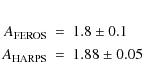
and
For the 16 stars, which were observed with FEROS and HARPS, we compared the
3.2 Age estimation
In the convective envelopes of F-M type stars, primordial lithium (Li I) is depleted as the star ages (e.g., Palla 2002). The amount of depletion depends also on the effective temperature of the star, which means that the equivalent width (EW) of Li I can only be compared among stars with the same effective temperatures, i.e., spectral type. To derive the dependency of Li I EW on age and spectral type, the measured mean Li I EW for different stellar associations with known age have been used. These associations are UMa (300 Myr), Pleiades (90 Myr), IC 2602 (30 Myr), TucHor (30 Myr),The age of the individual stars in our list has then been derived by comparing the EW of Li I at 6708 Å with this grid. For stars that are members of young stellar associations with known age range, the age derived by the Li I EW has been compared to the mean age of the associations. We find that the age estimates agree very well in all cases, confirming the validity of our approach.
3.3 Veiling
For accreting stars, veiling produces an additional continuum overlayed on the intrinsic stellar spectrum due to hot accretion spots on the stellar photosphere. This additional continuum alters the EW of spectral lines, as it changes the relative line depth (e.g., Appenzeller & Mundt 1989). Therefore, the veiling has to be determined in order to derive the pure photospheric EW of Li I.
In order to determine the veiling, theoretical spectra have
been computed for the respective stellar spectral types by using the
SPECTRUM package (Gray & Corbally 1994) together
with Kurucz atmosphere files (Kurucz 1993). These
theoretical spectra have been broadened to the ![]() of the star and veiled by adding a flat continuum.
The veiling of the target stars has then been determined using spectral
lines other than Li I in a 50 Å
window centred on the Li I feature
(6708 Å) by minimising the difference between the simulated
and the observed stellar spectrum. The EW of Li I
was then corrected by
of the star and veiled by adding a flat continuum.
The veiling of the target stars has then been determined using spectral
lines other than Li I in a 50 Å
window centred on the Li I feature
(6708 Å) by minimising the difference between the simulated
and the observed stellar spectrum. The EW of Li I
was then corrected by
where V is the measured veiling (Johns-Krull & Basri 1997).
Veiling also affects the colours of accreting stars, such that they
appear to be of earlier spectral type than they actually are. This is
because the boundary layer of the circumstellar disk, where the
accreted material is originating from, emits more light in the blue
part of the stellar spectrum (Hartigan et al. 1989). Thus,
due to an apparent shift to an earlier spectral type, this will
underestimate ![]() in Eq. (A.6).
The width of the CCF remains unchanged. With an unchanged CCF and
underestimation of
in Eq. (A.6).
The width of the CCF remains unchanged. With an unchanged CCF and
underestimation of ![]() due to a wrong ( b-
v), we therefore slightly overestimate the
due to a wrong ( b-
v), we therefore slightly overestimate the ![]() for accreting stars.
for accreting stars.
The maximum change in ![]() due to veiling can be estimated by using Eq. (A.6) and a shift
in spectral type from M0 to G0 (as an example of the effect of
veiling). We found this maximum effect on
due to veiling can be estimated by using Eq. (A.6) and a shift
in spectral type from M0 to G0 (as an example of the effect of
veiling). We found this maximum effect on ![]() to be 0.7 km s-1, which is
smaller than the uncertainty of our
to be 0.7 km s-1, which is
smaller than the uncertainty of our ![]() measurements, and, therefore, does not affect our results.
measurements, and, therefore, does not affect our results.
3.4 Signatures of accretion and disk presence
In order to analyse the measured ![]() for disk-braking mechanisms, we have to know the evolutionary state of
the circumstellar disks of our target stars. Furthermore, we have to
distinguish between accreting and non-accreting stars.
for disk-braking mechanisms, we have to know the evolutionary state of
the circumstellar disks of our target stars. Furthermore, we have to
distinguish between accreting and non-accreting stars.
To identify stars which are still accreting, the EW
and full width at 10% height (
![]() )
of the H
)
of the H![]() emission, as well as the EW of He I
at 5876 Å have been measured. All criteria have to be
fulfilled, because high stellar rotation broadens also the H
emission, as well as the EW of He I
at 5876 Å have been measured. All criteria have to be
fulfilled, because high stellar rotation broadens also the H![]() emission line.
emission line.
To distinguish between H![]() emission due to chromospheric activity and due to accretion of disk
material, the criteria by Appenzeller & Mundt (1989), and
Jayawardhana et al. (2006) have
both been investigated. According to Appenzeller & Mundt (1989) a
star is assumed to accrete when the EW of H
emission due to chromospheric activity and due to accretion of disk
material, the criteria by Appenzeller & Mundt (1989), and
Jayawardhana et al. (2006) have
both been investigated. According to Appenzeller & Mundt (1989) a
star is assumed to accrete when the EW of H![]() exceds 10 Å. In contrast, Jayawardhana et al. (2006) use
exceds 10 Å. In contrast, Jayawardhana et al. (2006) use
![]() and determine a value of 200 km s-1
(4.4 Å) as the accretion threshold.
and determine a value of 200 km s-1
(4.4 Å) as the accretion threshold.
The EW of H![]() has been widely used to identify accreting stars, but chromospherically
active stars can produce a comparable increase of the H
has been widely used to identify accreting stars, but chromospherically
active stars can produce a comparable increase of the H![]() EW. During accretion, H
EW. During accretion, H![]() emission also arises from ``hot spots'' on the stellar surface produced
by accreting disk material. The EW in both cases
can be comparable, because for late-type stars, the chromospheric H
emission also arises from ``hot spots'' on the stellar surface produced
by accreting disk material. The EW in both cases
can be comparable, because for late-type stars, the chromospheric H![]() emission is more prominent due to a diminished photosphere as compared
to hotter stars (e.g., White & Basri 2003). This
means, that the EW of H
emission is more prominent due to a diminished photosphere as compared
to hotter stars (e.g., White & Basri 2003). This
means, that the EW of H![]() due to chromospheric activity is much higher for cool stars and depends
on the spectral type of the stars. Therefore, no clear statement can be
made at which H
due to chromospheric activity is much higher for cool stars and depends
on the spectral type of the stars. Therefore, no clear statement can be
made at which H![]() EW a star accretes.
EW a star accretes.
A better discrimination between accreting and
chromospherically active stars can be made by measuring the
![]() of the emission feature. Emission due to an active chromosphere is
limited in amount by the saturation of the chromosphere and in width by
stellar rotation and non-thermal velocities of the chromosphere. White
& Basri (2003)
found that accreting stars tend to have
of the emission feature. Emission due to an active chromosphere is
limited in amount by the saturation of the chromosphere and in width by
stellar rotation and non-thermal velocities of the chromosphere. White
& Basri (2003)
found that accreting stars tend to have
![]() broader than 270 km s-1
(5.9 Å), whereas Jayawardhana et al. (2006) used
a less conservative threshold at 200 km s-1
(4.4 Å). For the purpose of this paper, the threshold from
Jayawardhana et al. (2006) has
been used to avoid missing accretors in this selection process.
broader than 270 km s-1
(5.9 Å), whereas Jayawardhana et al. (2006) used
a less conservative threshold at 200 km s-1
(4.4 Å). For the purpose of this paper, the threshold from
Jayawardhana et al. (2006) has
been used to avoid missing accretors in this selection process.
In addition, He I at
5876 Å has been investigated, because stellar rotation also
affects the ![]() .
The He I feature can be directly linked to
the accretion process of the star, because the luminosity of He I
correlates with the accretion luminosity (Fang et al. 2009, and
references herein). Other features, like [O I]
at 8446 Å cannot be used to identify the accretion process,
since it can be contaminated by the [O I]
feature of the circumstellar disk (Fang et al. 2009). All stars
identified as accretor candidates by the H
.
The He I feature can be directly linked to
the accretion process of the star, because the luminosity of He I
correlates with the accretion luminosity (Fang et al. 2009, and
references herein). Other features, like [O I]
at 8446 Å cannot be used to identify the accretion process,
since it can be contaminated by the [O I]
feature of the circumstellar disk (Fang et al. 2009). All stars
identified as accretor candidates by the H![]() criteria of Jayawardhana et al. (2006),
have also been searched for presence of He I.
We identified only those stars as accretors that fulfil both criteria,
criteria of Jayawardhana et al. (2006),
have also been searched for presence of He I.
We identified only those stars as accretors that fulfil both criteria,
![]() (Jayawardhana et al. 2006) and
the presence of He I. This results in 12
accretors in our sample, which are listed in Table 1.
(Jayawardhana et al. 2006) and
the presence of He I. This results in 12
accretors in our sample, which are listed in Table 1.
Accretion rates were then derived by computing the luminosity
of H![]() ,
H
,
H![]() ,
and He I, which correlates with the
accretion luminosity and applying Eq. (2) in Fang
et al. (2009).
,
and He I, which correlates with the
accretion luminosity and applying Eq. (2) in Fang
et al. (2009).
Information about the presence or absence of circumstellar disks and the type of disks has been adopted from Carpenter et al. (2009) for those stars in our sample which have been taken from the FEPS targets.
4 Results
Our results are compiled in Table 3. In this
table, we list the derived ![]() and its error in Cols. (3) and (4). The EW
of H
and its error in Cols. (3) and (4). The EW
of H![]() ,
its accuracy,
,
its accuracy, ![]() ,
EW of He I, and Veiling
are listed in Cols. (5) through (9). The Li I
measurements and the derived stellar ages are listed in
Cols. (10) to (13), and finally, the evolutionary state of the
circumstellar disk (if present) and the stellar association to which
the star belongs are listed in Cols. (14) and (15).
,
EW of He I, and Veiling
are listed in Cols. (5) through (9). The Li I
measurements and the derived stellar ages are listed in
Cols. (10) to (13), and finally, the evolutionary state of the
circumstellar disk (if present) and the stellar association to which
the star belongs are listed in Cols. (14) and (15).
4.1 Age
Almost all of our target stars show the Li I feature at 6708 Å, thus confirming their youth. We find a typical detection limit for the Li I feature of 2 mÅ in spectra with a SNR > 10 around 6700 Å. In spectra with a SNR<10, we were not able to measure the EW of Li I. The EW of Li I was not corrected for the possible blend with a nearby Fe I feature, because the correction would be smaller than our measurement accuracy (cf. Soderblom 1993).
The measured EW of Li I are listed in Cols. (10) and (11) of Table 3 and were used to derive the age of the individual stars as described in Sect. 3.2. The accuracy of this method is typically 10-50%.
The resulting age distribution is shown in Fig. 2. The histogram
has a strong peak at 30 Myr, which is due to the selection
effect towards stars in associations with these ages (from Zuckerman
& Song 2004).
Note that the age estimate stated in the literature was already a
selection criterion for this source sample (see Sect. 2.1). In
total, we found 5 stars which are most likely older than the
Hyades (
![]() 600 Myr), and 43
stars that are younger than 10 Myr.
600 Myr), and 43
stars that are younger than 10 Myr.
In 10 stars, we could not detect the Li I feature. Of these, 2 stars (TYC 9129-1361-1 and HD 21411) have a sufficient SNR, but the Li I feature is below the detection limit of 2 mÅ. The spectra of 8 stars (HD 43989, HD 201219, HD 201989, HD 205905, HD 209253, HD209779, HD 212291, and HD 225213) have an insufficient SNR<10, and no lithium feature could be identified and measured. These 8 stars are marked with ``n/a'' in Table 3 (Col. 10).
![\begin{figure}
\par\includegraphics[width=8.5cm,clip]{14453fig2.eps}
\vspace*{4mm}
\end{figure}](/articles/aa/full_html/2010/09/aa14453-10/img42.png)
|
Figure 2: Distribution of stellar ages within our sample, derived from the measured EW of Li I at 6708 Å (see Sects. 3.2 and 4.1). |
| Open with DEXTER | |
4.2 Evolutionary state of the stars
Table 1:
EW of H![]() ,
,
![]() ,
EW of He I, accretion
rates
,
EW of He I, accretion
rates ![]() ,
and
,
and ![]() for accretor candidates. Close binary or multiple stars are marked with
for accretor candidates. Close binary or multiple stars are marked with
![]() .
.
All stars with EW of He I > 20 mÅ
(detection threshold in our spectra) and
![]() 4.4 Å
(Sect. 3.4)
are classified here as accretors. The accretors in this sub-sample are
DI Cha, TW Hya, GW Ori, CR Cha,
V2129 Oph, GQ Lup, IM Lup, DoAr 44,
EM* SR 9, HBC 603,
V1121 Oph, and MP Mus. For our analysis, we excluded
GW Ori because it is a close binary star (Ghez et al.
1997). The
accretion rates have been calculated following Fang et al. (2009) with a
typical computational accuracy of 15%. For IM Lup, we were not
able to derive an accretion rate because the measured EW
of H
4.4 Å
(Sect. 3.4)
are classified here as accretors. The accretors in this sub-sample are
DI Cha, TW Hya, GW Ori, CR Cha,
V2129 Oph, GQ Lup, IM Lup, DoAr 44,
EM* SR 9, HBC 603,
V1121 Oph, and MP Mus. For our analysis, we excluded
GW Ori because it is a close binary star (Ghez et al.
1997). The
accretion rates have been calculated following Fang et al. (2009) with a
typical computational accuracy of 15%. For IM Lup, we were not
able to derive an accretion rate because the measured EW
of H![]() ,
H
,
H![]() and He I could not be fitted by the assumed
accretion model. In addition to the accretors, 5 more stars also show
and He I could not be fitted by the assumed
accretion model. In addition to the accretors, 5 more stars also show
![]() over the threshold of 4.4 Å, but no He I
has been found in the spectra of these stars. For these stars, the H
over the threshold of 4.4 Å, but no He I
has been found in the spectra of these stars. For these stars, the H![]() emission is likely due to chromospheric activity and broadened by fast
rotation or an undiscovered close binary. These 5 stars are
HT Lup, HD 3221, CP-72 2713, TWA 6,
and TWA 5. We list all 17 stars with a
emission is likely due to chromospheric activity and broadened by fast
rotation or an undiscovered close binary. These 5 stars are
HT Lup, HD 3221, CP-72 2713, TWA 6,
and TWA 5. We list all 17 stars with a
![]() Å,
accretors and non-accretors, in Table 1.
Å,
accretors and non-accretors, in Table 1.
4.3 Projected rotational velocities
![\begin{figure}
\par\includegraphics[width=8.5cm,clip]{14453fig3.eps} %
\vspace*{4mm}
\end{figure}](/articles/aa/full_html/2010/09/aa14453-10/img52.png)
|
Figure 3:
Distribution of |
| Open with DEXTER | |
Table 2:
Sub-samples used to investigate the dependence of ![]() on the evolutionary state of the stars.
on the evolutionary state of the stars.
The ![]() derived from the FEROS or HARPS spectra for all stars are listed in
Col. (3) of Table 3. The lower
limit of the
derived from the FEROS or HARPS spectra for all stars are listed in
Col. (3) of Table 3. The lower
limit of the ![]() measurements has been calculated by using artificially broadened
theoretical spectra to be 2 km s-1
for our data. Thus, for all stars in our sample, the line broadening
due to rotation exceeds the instrumental broadening. Figure 3 shows the
distribution of
measurements has been calculated by using artificially broadened
theoretical spectra to be 2 km s-1
for our data. Thus, for all stars in our sample, the line broadening
due to rotation exceeds the instrumental broadening. Figure 3 shows the
distribution of ![]() for all stars in our sample. We fitted all histograms with a
for all stars in our sample. We fitted all histograms with a ![]() -normal
distribution function using a
-normal
distribution function using a ![]() minimization algorithm. The fit to the
minimization algorithm. The fit to the ![]() distribution of all stars peaks at 7.8
distribution of all stars peaks at 7.8 ![]() 1.2 km s-1
with a width of 9 km s-1. We
find that 70% of our stars have
1.2 km s-1
with a width of 9 km s-1. We
find that 70% of our stars have ![]() 30 km s-1.
However, a sub-sample of 59 stars was biased towards slow
rotators due to our selection (see Sect. 2.1). For
our analysis of
30 km s-1.
However, a sub-sample of 59 stars was biased towards slow
rotators due to our selection (see Sect. 2.1). For
our analysis of ![]() as function of stellar mass (Sect. 4.3.1), we
therefore excluded those 59 stars which have been initially
chosen to have
as function of stellar mass (Sect. 4.3.1), we
therefore excluded those 59 stars which have been initially
chosen to have ![]() 30 km s-1.
However, we have to include them again in Sect. 4.3.2 for the
analysis of
30 km s-1.
However, we have to include them again in Sect. 4.3.2 for the
analysis of ![]() as a function of the evolutionary state, because these stars are the
youngest in our sample. Our analysis also revealed that 8 of these
59 stars have in fact
as a function of the evolutionary state, because these stars are the
youngest in our sample. Our analysis also revealed that 8 of these
59 stars have in fact ![]() 30 km s-1.
These stars are CD-78 24, GW Ori, HD 42270,
CR Cha, Di Cha, T Cha, HT Lup, and
HD 220054. The
30 km s-1.
These stars are CD-78 24, GW Ori, HD 42270,
CR Cha, Di Cha, T Cha, HT Lup, and
HD 220054. The ![]() measurements for the stars in our sample are important to select target
stars for radial velocity planet searches around young stars, since
sufficient RV accuracy can only be achieved for slow rotators (
measurements for the stars in our sample are important to select target
stars for radial velocity planet searches around young stars, since
sufficient RV accuracy can only be achieved for slow rotators (
![]() km s-1).
The 14 identified binary or multiple systems (see
Sect. 4.5)
have also been excluded from our analysis.
km s-1).
The 14 identified binary or multiple systems (see
Sect. 4.5)
have also been excluded from our analysis.
4.3.1 v sin i as a function of stellar mass
The rotational evolution of a star depends on its magnetic activity,
which is coupled to the stellar mass (e.g., Attridge & Herbst 1992; Palla 2002, and
references herein). Lower-mass stars tend to have higher magnetic
activity due to the deeper convection zones than higher-mass stars,
because the stellar magnetic field is driven by the convective zone.
Thus, due to the higher magnetic activity, lower-mass stars are
therefore expected to rotate slower than higher-mass stars. To examine
this dependency, we followed Nguyen et al. (2009) and
divided our sample into two sub-samples of spectral types F-K (higher
mass) and M (lower mass). In order to be not affected by possible age
effects, we selected for this test only stars which are younger than
20 Myr, resulting in sub-samples of 21 F-K type stars and 12
M-type stars. For the F-K type stars, we find a weighted mean of
![]() km s-1
and for M-type stars
km s-1
and for M-type stars
![]() km s-1.
This difference is small, but significant and confirms the finding of
Nguyen et al. (2009),
that late-type, lower-mass stars rotate on average slower than
earlier-type, higher-mass stars. Note, that all stars in our sample
have
km s-1.
This difference is small, but significant and confirms the finding of
Nguyen et al. (2009),
that late-type, lower-mass stars rotate on average slower than
earlier-type, higher-mass stars. Note, that all stars in our sample
have ![]() ,
such that we are not able to probe the higher rotation rates of stars
with
,
such that we are not able to probe the higher rotation rates of stars
with ![]() as found in the Orion Nebular Cluster (Attridge & Herbst 1992).
as found in the Orion Nebular Cluster (Attridge & Herbst 1992).
4.3.2 v sin i as a function of evolutionary state
To search for evidence of disk-braking and rotational spin-up in our
sample, we analysed the ![]() distributions of the 5 sub-samples described in Sect. 4.2. Note that
these sub-samples have been created independently of the mass of the
individual stars and we only compare different evolutionary stages. The
distributions of the 5 sub-samples described in Sect. 4.2. Note that
these sub-samples have been created independently of the mass of the
individual stars and we only compare different evolutionary stages. The
![]() distributions
of the sub-samples have been fitted with a
distributions
of the sub-samples have been fitted with a ![]() -normal
distribution function. The resulting mean
-normal
distribution function. The resulting mean
![]() and widths
and widths ![]() are listed in Cols. 6 and 7 of Table 2. Since
sub-samples (iv) and (v) represent similar
evolutionary states, we combined them for further analysis. The
distribution histograms together with the fits are shown in
Fig. 4.
are listed in Cols. 6 and 7 of Table 2. Since
sub-samples (iv) and (v) represent similar
evolutionary states, we combined them for further analysis. The
distribution histograms together with the fits are shown in
Fig. 4.
![\begin{figure}
\par\includegraphics[width=8.5cm,clip]{14453fig4a.eps}\hspace{2mm...
...\includegraphics[width=8.5cm,clip]{14453fig4b.eps} %\vspace*{4mm}
\end{figure}](/articles/aa/full_html/2010/09/aa14453-10/img73.png)
|
Figure 4:
Distribution of |
| Open with DEXTER | |
As a result, we find that accretors are slow rotators. Furthermore,
stars in sub-sample (ii) with non-accreting and optically thick disks
rotate on average faster compared to accreting stars and stars at later
evolutionary stages. However, the ![]() distribution for these stars shows a large spread of rotation
velocities. Stars older than 30 Myr rotate again slower on
average, but with a long tail in the distribution towards individual
fast rotators. This general trend conforms with the well-known picture
that rotational spin-up of contracting Pre-Main-Sequence stars is
compensated by efficient braking mechanisms during the accretion phase.
At the end of the accretion phase, there is no or less efficient
braking, such that a rotational spin-up occurs. In later evolutionary
stages on the ZAMS, other braking mechanisms are efficient. These
mechanisms depend on different disk-braking and contraction times of
the individual stars, thus leading to several individual fast rotators.
Note that other surveys of stellar rotation in young open clusters
found a larger spread in rotation of stars with an age of
30 Myr than we found in our data and rotational spin-down has
been found for stars older than 30 Myr (e.g., Allain 1998). This
difference is possibly due to a lower number of stars in sub-sample
(iii) and the error in age estimation. However, the general trend in
our data is consistent with the findings of other surveys (e.g.,
Scilia-Aguilar et al. 2004; Lamm et al. 2005).
distribution for these stars shows a large spread of rotation
velocities. Stars older than 30 Myr rotate again slower on
average, but with a long tail in the distribution towards individual
fast rotators. This general trend conforms with the well-known picture
that rotational spin-up of contracting Pre-Main-Sequence stars is
compensated by efficient braking mechanisms during the accretion phase.
At the end of the accretion phase, there is no or less efficient
braking, such that a rotational spin-up occurs. In later evolutionary
stages on the ZAMS, other braking mechanisms are efficient. These
mechanisms depend on different disk-braking and contraction times of
the individual stars, thus leading to several individual fast rotators.
Note that other surveys of stellar rotation in young open clusters
found a larger spread in rotation of stars with an age of
30 Myr than we found in our data and rotational spin-down has
been found for stars older than 30 Myr (e.g., Allain 1998). This
difference is possibly due to a lower number of stars in sub-sample
(iii) and the error in age estimation. However, the general trend in
our data is consistent with the findings of other surveys (e.g.,
Scilia-Aguilar et al. 2004; Lamm et al. 2005).
To search for indications of disk-braking, we compared the ![]() of stars in sub-sample (i) with the accretion rates listed in
Table 1.
Disk-braking mechanisms depend on a magnetic connection between the
star and its circumstellar disk and therefore on the accretion rate of
the star. Furthermore, stellar age and disk lifetimes are expected to
have an impact on disk-braking, since the amount of time spent for
rotational braking by the disk (disk-braking time; e.g., Nguyen
et al. 2009)
determines the resulting stellar rotation velocity. However, this also
depends on the initial rotational conditions of the star-forming
region. The
of stars in sub-sample (i) with the accretion rates listed in
Table 1.
Disk-braking mechanisms depend on a magnetic connection between the
star and its circumstellar disk and therefore on the accretion rate of
the star. Furthermore, stellar age and disk lifetimes are expected to
have an impact on disk-braking, since the amount of time spent for
rotational braking by the disk (disk-braking time; e.g., Nguyen
et al. 2009)
determines the resulting stellar rotation velocity. However, this also
depends on the initial rotational conditions of the star-forming
region. The ![]() distribution for accretors in sub-sample (i) can be due to a
combination of these effects, in which the amount of time spent for
disk-braking is dominant, because the two youngest accretors
(DI Cha and CR Cha) rotate faster than the other
accretors independent of their accretion rate. This gets also supported
by other surveys (e.g., Joergens & Guenther 2001;
Scilia-Aguilar et al. 2004; Lamm et al. 2005; Jayawardhana
et al. 2006;
Nguyen et al. 2009).
A larger survey of stars in different star-forming regions, measuring
the age and accretion rates, would be necessary to study the dependence
of stellar rotation on
distribution for accretors in sub-sample (i) can be due to a
combination of these effects, in which the amount of time spent for
disk-braking is dominant, because the two youngest accretors
(DI Cha and CR Cha) rotate faster than the other
accretors independent of their accretion rate. This gets also supported
by other surveys (e.g., Joergens & Guenther 2001;
Scilia-Aguilar et al. 2004; Lamm et al. 2005; Jayawardhana
et al. 2006;
Nguyen et al. 2009).
A larger survey of stars in different star-forming regions, measuring
the age and accretion rates, would be necessary to study the dependence
of stellar rotation on ![]() further.
further.
4.4 Stellar rotation periods
For stars for which accurate measurements of
![]() ,
absolute magnitude, and bolometric correction are available (e.g., from
Weise 2007;
Flower 1996),
we estimated the stellar radius
,
absolute magnitude, and bolometric correction are available (e.g., from
Weise 2007;
Flower 1996),
we estimated the stellar radius
![]() following Valenti & Fischer (2005).
An upper limit to the rotational period of the star can then be derived
from the estimated radius by using:
following Valenti & Fischer (2005).
An upper limit to the rotational period of the star can then be derived
from the estimated radius by using:
| (4) |
The resulting distribution of rotational periods for the whole sample is shown in Fig. 5. The distribution of
However, because of the uncertainties introduced by the
assumptions used to calculate the radii of the stars, no further
analysis of ![]() has been done, like, e.g. for
has been done, like, e.g. for ![]() in Sect. 4.3.2.
in Sect. 4.3.2.
4.5 Binary and multiple systems
From the CCFs, we are also able to identify double-lined spectroscopic binaries (SB2). We clearly identified 9 stars to be SB2s (GJ 3323, TWA 4, TYC 6604-118-1, TYC 9129-1361-1, HD 124784, HD 139498, HD 140374, HD 141521, and HD 155555), such that our total list in Table 3 consists of 229 stars. All 9 stars have already been known as multiple systems. For all 9 SB2s, the CCF of each component has been analysed separately and the appropriateIn addition to the clearly identified SB2 stars, more known multiple stars are in our sample: TWA 5, GW Ori, DI Cha, and HT Lup (Jayawardhana 2006; Ghez et al. 1997; Mathieu et al. 1995). However, the components of these systems cannot be distinguished in the CCFs to analyse them separately, because they are single-lined binaries (SB1). A few more SB1 systems might be found in our sample when the analysis of multiple epoch RV data is finished, but this is beyond the scope of this paper.
![\begin{figure}
\par\includegraphics[width=9cm,clip]{14453fig5.eps}
\end{figure}](/articles/aa/full_html/2010/09/aa14453-10/img79.png)
|
Figure 5:
Distribution of the stellar rotation period
|
| Open with DEXTER | |
5 Summary and conclusions
We analysed 229 young and nearby stars for their projected
rotational velocity ![]() ,
stellar age, and accretion signatures. The stars were part of our
initial RV planet search target list in the SERAM project and have been
observed with FEROS at the 2.2 m MPG/ESO telescope and HARPS
at the 3.6 m telescope in La Silla, Chile. For stars showing
broad H
,
stellar age, and accretion signatures. The stars were part of our
initial RV planet search target list in the SERAM project and have been
observed with FEROS at the 2.2 m MPG/ESO telescope and HARPS
at the 3.6 m telescope in La Silla, Chile. For stars showing
broad H![]() emission, we checked other accretion indicators, like the EW
of He I at 5876 Å, to identify
those stars that still accrete material from a circumstellar disk. For
these stars, the veiling has also been measured. The age of the stars
has been derived from the EW of Li I
at 6708 Å.
emission, we checked other accretion indicators, like the EW
of He I at 5876 Å, to identify
those stars that still accrete material from a circumstellar disk. For
these stars, the veiling has also been measured. The age of the stars
has been derived from the EW of Li I
at 6708 Å.
We calculated ![]() of our 220 target stars and 9 spectroscopic companions by measuring the
width of the CCF of the stellar spectra. To do this, we
cross-correlated the stellar spectra with theoretical templates of
similar spectral type. The CCF has been fitted with a Gaussian and the
conversion to
of our 220 target stars and 9 spectroscopic companions by measuring the
width of the CCF of the stellar spectra. To do this, we
cross-correlated the stellar spectra with theoretical templates of
similar spectral type. The CCF has been fitted with a Gaussian and the
conversion to ![]() was done with our new calibration (Eq. (A.6)) for both
FEROS and HARPS spectra.
was done with our new calibration (Eq. (A.6)) for both
FEROS and HARPS spectra.
The main conclusions from this work can be summarized as follows:
- The mean stellar age of our sample is 30 Myr with a spread (width of Gaussian fit) of 20 Myr. 43 stars are younger than 10 Myr.
- The distribution of
 for all target stars peaks at 7.8
 1.2 km s-1,
with the vast majority having projected rotational velocities
<30 km s-1.
1.2 km s-1,
with the vast majority having projected rotational velocities
<30 km s-1.
- We found indication for rotational braking due to
disk-locking, because the accreting stars in our sample rotate
significantly slower (
 km s-1)
than the non-accreting stars with more evolved disks (
km s-1)
than the non-accreting stars with more evolved disks (
 km s-1).
The only 2 fast rotating (
km s-1).
The only 2 fast rotating (
 km s-1)
accretors in our sample are DI Cha and CR Cha. This
might point to differences in time spent for disk-braking or to
different initial conditions in different star formation regions, but
the significance of this statement is hampered by low number
statistics.
km s-1)
accretors in our sample are DI Cha and CR Cha. This
might point to differences in time spent for disk-braking or to
different initial conditions in different star formation regions, but
the significance of this statement is hampered by low number
statistics.
- This
evolution also provides indication that stars undergo rotational
spin-up after being decoupled from their circumstellar disk and
evolving along the Pre-Main-Sequence track. For more evolved stars with
debris or no disks and an age >30 Myr,
 decreases again to 10 1 km s-1.
We conclude that these stars have been rotationally braked on the ZAMS,
e.g., by magnetic winds.
decreases again to 10 1 km s-1.
We conclude that these stars have been rotationally braked on the ZAMS,
e.g., by magnetic winds.
- We estimated the maximum rotational period of our target
stars. The period distribution of the whole sample peaks at
2.5 0.3 days,
a similar result as found for young stars by Cieza & Biliber (2007).
- Due to disk-braking, young and accreting stars can rotate
sufficiently slow to serve as suitable targets for RV planet searches,
since the accuracy of radial velocity measurements depends on the
stellar .
When accretion ends after
 5-10 Myr
and the stars decouple from their disk, they tend to spin up as they
contract, such that they are usually no longer suitable for precise RV
measurements. This changes only when the stars arrive on the ZAMS and
are slowed down again by wind braking at ages of 30 Myr.
5-10 Myr
and the stars decouple from their disk, they tend to spin up as they
contract, such that they are usually no longer suitable for precise RV
measurements. This changes only when the stars arrive on the ZAMS and
are slowed down again by wind braking at ages of 30 Myr.
This research has made use of the SIMBAD database, operated at CDS, Strasbourg, France. Based on observations made with the European Southern Observatory telescopes obtained from the ESO/ST-ECF Science Archive Facility. We gratefully thank M. Fang for the calculation of the accretion rates, R. Mundt for helpful discussions, the unknown Referee for his comments, and the staff at La Silla, Chile for their support. We want to thank the observers E. Meyer, M. Zechmeister, M. Lendl, V. Joergens, J. Datson, T. Schulze-Hartung, D. Fedele, J. Carson and A. Müller.
Appendix A: Calibration of v sin i
In this Appendix, the calibration for the ![]() measurements in Sect. 3.1
is presented. The
measurements in Sect. 3.1
is presented. The ![]() can be calculated from the width of the CCF
can be calculated from the width of the CCF
![]() by using
by using
where A is a coupling constant and
The coupling constant A and ![]() can be calibrated independently of each other, since the quantity A
only depends on instrumental and numerical parameters and the quantity
can be calibrated independently of each other, since the quantity A
only depends on instrumental and numerical parameters and the quantity ![]() depends on intrinsic stellar effects. On the other hand, each is needed
to calibrate the other variable. To be able to calibrate A,
depends on intrinsic stellar effects. On the other hand, each is needed
to calibrate the other variable. To be able to calibrate A,
![]() has been
taken as the width of the unbroadenend artifical spectra (see
Sect. A.1).
The resulting A has been used to calibrate
has been
taken as the width of the unbroadenend artifical spectra (see
Sect. A.1).
The resulting A has been used to calibrate ![]() (Sect. A.2)
with spectra of slow rotating stars with different effective
temperatures. As a cross-check,
(Sect. A.2)
with spectra of slow rotating stars with different effective
temperatures. As a cross-check, ![]() computed in Sect. A.2
has been iteratively used to recalculate A
(Sect. A.1),
which yielded the same results for A.
computed in Sect. A.2
has been iteratively used to recalculate A
(Sect. A.1),
which yielded the same results for A.
A.1 Calibration of the coupling constant A
The coupling constant A has been derived in a similar way as described
by Queloz et al. (1998). For this analysis, theoretical
spectra have been cross-correlated with an appropriate template. A
synthetic stellar spectrum with effective temperature of
5750 K and ![]() dex
has been produced from Kurucz models (Kurucz 1993), using the
program SPECTRUM (Gray & Corbally 1994). This has
been done to have the best agreement with the used template for G-type
stars. In a first step, the theoretical spectrum has been convolved
with a Gaussian-shape instrumental profile matching that of FEROS or
HARPS, respectively. Then, the theoretical spectrum with the
instrumental profile has been broadened to
dex
has been produced from Kurucz models (Kurucz 1993), using the
program SPECTRUM (Gray & Corbally 1994). This has
been done to have the best agreement with the used template for G-type
stars. In a first step, the theoretical spectrum has been convolved
with a Gaussian-shape instrumental profile matching that of FEROS or
HARPS, respectively. Then, the theoretical spectrum with the
instrumental profile has been broadened to
![]() ,
5, 10, 15, 20, 25 and 30 km s-1 and the
respective CCF has been calculated by using MACS. The widths of the CCF
obtained by a Gaussian fit,
,
5, 10, 15, 20, 25 and 30 km s-1 and the
respective CCF has been calculated by using MACS. The widths of the CCF
obtained by a Gaussian fit,
![]() ,
are listed in Table A.1.
The effective line width of a non-rotating star,
,
are listed in Table A.1.
The effective line width of a non-rotating star,
![]() ,
has been adopted to be equal to the width of the CCF with
,
has been adopted to be equal to the width of the CCF with
![]() .
.
The coupling constant A was then
determined as the weighted mean of the A-values
derived for the CCFs with different ![]() ,
using Eq. (A.1).
We derive
,
using Eq. (A.1).
We derive
| (A.2) |
and
| (A.3) |
In both cases, the cross-check by using the
Table A.1: Calibration of A.
![\begin{figure}
\par\includegraphics[width=8.5cm,clip]{14453fig6.eps}
\end{figure}](/articles/aa/full_html/2010/09/aa14453-10/img128.png)
|
Figure A.1:
Calibration of |
| Open with DEXTER | |
The scatter of A around the adopted weighted mean value is due to the fact that the shape of rotationally broadened spectral lines is no longer well represented by a Gaussian (e.g., Gray 1992). Thus, the scatter has been introduced by the imperfect matching of the Gaussian fitting function. This behaviour only affects the measurement of the width of the CCF but not the determination of the minimum position, since the CCF of the theoretical spectra is symmetric. In order to test, whether other fitting functions describe the resulting CCF better, several line-profile functions have been used, like an additionally broadened Gaussian. This function has been adopted from Hirano et al. (2010). They describe the stellar rotation profile by a Gaussian, which is then convolved with the first Gaussian used to describe the unbroadened spectral line.
As a result, measurements with all fitting functions yielded the same mean value for A and the scatter around it is not significantly reduced compared to a single Gaussian fit. Thus, an ideal fitting function for a rotationally broadened CCF is not yet existent.
A.2 Calibration of 
In order to correctly measure the projected rotational velocity ![]() of a target and to disentangle it from the intrinsic and instrumental
broadening effects,
of a target and to disentangle it from the intrinsic and instrumental
broadening effects, ![]() has to be known. The instrumental broadening effects should be
independent of stellar properties of the observed star, while the
intrinsic stellar line broadening depends strongly on
has to be known. The instrumental broadening effects should be
independent of stellar properties of the observed star, while the
intrinsic stellar line broadening depends strongly on
![]() ,
due to Doppler broadening. From the Maxwellian most likely velocity of
atoms in thermal motion,
,
due to Doppler broadening. From the Maxwellian most likely velocity of
atoms in thermal motion,
![]() ,
and from the relation of the Doppler wavelength shift to this velocity,
,
and from the relation of the Doppler wavelength shift to this velocity,
![]() ,
it follows that
,
it follows that
Here
Table A.2:
Calibration stars for ![]() ,
sorted by ( b- v).
,
sorted by ( b- v).
Since not all stars have reliable measurements of
![]() ,
but colours, like ( b-
v) are available and can directly be linked to
,
but colours, like ( b-
v) are available and can directly be linked to
![]() ,
the relation of line broadening with ( b- v)
has been investigated. According to Flower (1996), the
relation between ( b-
v) and
,
the relation of line broadening with ( b- v)
has been investigated. According to Flower (1996), the
relation between ( b-
v) and ![]() for main-sequence stars and giants is linear within the region of
interest of 0<( b-
v)<1.6, such that
for main-sequence stars and giants is linear within the region of
interest of 0<( b-
v)<1.6, such that
holds. Hence, we can use
to fit the data. In order to determine this relation, slowly rotating stars have been observed with FEROS at the 2.2 m MPG/ESO telescope in La Silla, Chile in 2003 and 2004 and with HARPS at the 3.6 m telescope in La Silla, Chile in 2008 and 2009, see Table A.2.
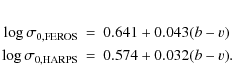
For FEROS data, the coefficients in Eq. (A.6) are
![]() ,
,
![]() ,
and for HARPS data the coefficients are
,
and for HARPS data the coefficients are
![]() and
and ![]() .
.
References
- Allain, S. 1998, A&A, 333, 629 [NASA ADS] [Google Scholar]
- Appenzeller, I., & Mundt, R. 1989, A&ARv, 1, 291 [NASA ADS] [CrossRef] [Google Scholar]
- Armitage, P. J., & Clarke, C. J. 1996, MNRAS, 280, 458 [NASA ADS] [Google Scholar]
- Attridge, J. M., & Herbst, W. 1992, ApJ, 398, L61 [NASA ADS] [CrossRef] [Google Scholar]
- Baranne, A., Mayor, M., & Poncet, J. L. 1979, Vistas Astron., 23, 279 [NASA ADS] [CrossRef] [Google Scholar]
- Baranne, A., Queloz, D., Mayor, M., et al. 1996, A&AS, 119, 373 [NASA ADS] [CrossRef] [EDP Sciences] [Google Scholar]
- Benz, W., & Mayor, M. 1984, A&A, 138, 183 [NASA ADS] [Google Scholar]
- Bodenheimer, P. 1989, NATO ASIC Proc. Theory of Accretion Disks, 290, 75 [NASA ADS] [Google Scholar]
- Bodenheimer, P. 1995, ARA&A, 33, 199 [NASA ADS] [CrossRef] [Google Scholar]
- Bouvier, J. 1993, The ESO Messenger, 71, 21 [NASA ADS] [Google Scholar]
- Bouvier, J. 1995, MmSAI, 66, 341 [NASA ADS] [Google Scholar]
- Bouwman, J., Lawson, W. A., Dominik, C., et al. 2006, ApJ, 653, L57 [NASA ADS] [CrossRef] [Google Scholar]
- Brown, J. M., Blake, G. A., Dullemond, C. P., et al. 2007, ApJ, 664, L107 [NASA ADS] [CrossRef] [Google Scholar]
- Camenzind, M. 1990, Rev. Mod. Astron., 3, 234 [Google Scholar]
- Carpenter, J. M., Bouwman, J., Silverstone, M. D., et al. 2008, ApJS, 179, 423 [NASA ADS] [CrossRef] [Google Scholar]
- Carpenter, J. M., Bouwman, J., Mamajek, E. E., et al. 2009, ApJS, 181, 197 [NASA ADS] [CrossRef] [Google Scholar]
- Chen, C. H., Patten, B. M., Werner, M. W., et al. 2005, ApJ, 634, 1372 [NASA ADS] [CrossRef] [Google Scholar]
- Cieza, L., & Biliber, N. 2007, ApJ, 671, 605 [NASA ADS] [CrossRef] [Google Scholar]
- Fallscheer, C., & Herbst, W. 2006, ApJ, 647, L155 [NASA ADS] [CrossRef] [Google Scholar]
- Fang, M., van Boeckel, R., Wang, W., et al. 2009, A&A, 504, 461 [NASA ADS] [CrossRef] [EDP Sciences] [Google Scholar]
- Flower, P. J. 1996, ApJ, 469, 355 [NASA ADS] [CrossRef] [Google Scholar]
- Gautier, T. N. III, Rebull, L. M., Stapelfeldt, K. R., et al. 2008, ApJ, 683, 813 [NASA ADS] [CrossRef] [Google Scholar]
- Ghez, A. M., McCarthy, D. W., Patience, J. L., & Beck, T. L. 1997, ApJ, 481, 378 [NASA ADS] [CrossRef] [Google Scholar]
- Gray, D. F. 1992, The Observation and Analysis of Stellar Photospheres, 2nd edn. (Cambridge University Press) [Google Scholar]
- Gray, D. F., & Toner, C. G. 1986, ApJ, 310, 277 [NASA ADS] [CrossRef] [Google Scholar]
- Gray, R. O., & Corbally, C. J. 1994, AJ, 107, 742 [NASA ADS] [CrossRef] [Google Scholar]
- Hartigan, P., Hartmann, L., Kenyon, S., Hewett, R., & Stauffer, J. 1989, ApJS, 70, 899 [NASA ADS] [CrossRef] [Google Scholar]
- Hartmann, L. 2002, ApJ, 566, L29 [NASA ADS] [CrossRef] [Google Scholar]
- Herbst, W., & Mundt, R. 2005, ApJ, 633, 967 [NASA ADS] [CrossRef] [Google Scholar]
- Herbst, W., Bailer-Jones, C. A. L., Mundt, R., et al. 2002, A&A, 396, 513 [NASA ADS] [CrossRef] [EDP Sciences] [Google Scholar]
- Herbst, W., Eislöffel, J., Mundt, R., & Scholz, A. 2007, Protostars and Planets V, 297 [Google Scholar]
- Herbst, W., Bailer-Jones, C. A. L., & Mundt, R. 2001, ApJ, 554, 197 [Google Scholar]
- Hirano, T., Suto, Y., Taruya, A., et al. 2010, ApJ, 709, 458 [NASA ADS] [CrossRef] [Google Scholar]
- Jayawardhana, R., Coffey, J., Scholz, A., et al. 2006, ApJ, 648, 1206 [NASA ADS] [CrossRef] [Google Scholar]
- Joergens, V., & Guenther, E. 2001, A&A, 379, L9 [NASA ADS] [CrossRef] [EDP Sciences] [Google Scholar]
- Johns-Krull, C. M., & Basri, G. 1997, ApJ, 474, 433 [NASA ADS] [CrossRef] [Google Scholar]
- Kaufer, A., Stahl, O., Tubbesing, S., et al. 1999, The ESO Messenger, 95, 8 [NASA ADS] [Google Scholar]
- Kaufer, A., Stahl, O., Tubbesing, S., et al. 2000, SPIE, 4008, 459 [NASA ADS] [Google Scholar]
- Kessler-Silacci, J., Augereau, J. C., Dullemond, C. P., et al. 2006, ApJ, 639, 275 [NASA ADS] [CrossRef] [Google Scholar]
- Köhler, R. 2001, AJ, 122, 3325 [NASA ADS] [CrossRef] [Google Scholar]
- Königl, A. 1991, ApJ, 370, L39 [NASA ADS] [CrossRef] [Google Scholar]
- Kurucz, R. L. 1993, CD-ROM 13, ATLAS9 Stellar Atmosphere Programs and 2 km s-1 Grid (Cambridge: Smithsonian Astrophys. Obs.) [Google Scholar]
- Lamm, M. H., Mundt, R., Bailer-Jones, C. A. L., & Herbst, W. 2005, A&A, 430, 1005 [NASA ADS] [CrossRef] [EDP Sciences] [Google Scholar]
- Launhardt, R., Queloz, D., Henning, Th., et al. 2008, SPIE, 7013, 76 [NASA ADS] [Google Scholar]
- Lommen, D., Wright, C. M., Maddison, S. T., et al. 2007, A&A, 462, 211 [NASA ADS] [CrossRef] [EDP Sciences] [Google Scholar]
- López-Santiago, J., Montes, D., Crespo-Chacón, I., & Fernández-Figueroa, M. J. 2006, ApJ, 643, 1160 [NASA ADS] [CrossRef] [Google Scholar]
- Low, F. J., Smith, P. S. Werner, M., et al. 2005, ApJ, 631, 1170 [NASA ADS] [CrossRef] [Google Scholar]
- Makarov, V. V., & Fabricius, C. 2001, A&A, 368, 866 [NASA ADS] [CrossRef] [EDP Sciences] [Google Scholar]
- Makidon, R. B., Rebull, L. M., Strom, S. E., et al. 2004, AJ, 127, 2228 [NASA ADS] [CrossRef] [Google Scholar]
- Mamajek, E. E., Meyer, M. R., & Liebert, J. 2002, AJ, 124, 1670 [NASA ADS] [CrossRef] [Google Scholar]
- Mamajek, E. E., Meyer, M. R., Hinz, P. M., et al. 2004, ApJ, 612, 496 [NASA ADS] [CrossRef] [Google Scholar]
- Mathieu, R. D., Adams F. C., & Latham, D. W. 1991, AJ, 101, 2184 [NASA ADS] [CrossRef] [Google Scholar]
- Matt, S., & Pudritz, R. E. 2005, ApJ, 632, L135 [NASA ADS] [CrossRef] [Google Scholar]
- Matt, S., & Pudritz, R. E. 2008, 14th Cambridge Workshop on Cool Stars, 384, 339 [Google Scholar]
- Mayor, M., Pepe, F., Queloz, D., et al. 2003, The Eso Messenger, 114, 20 [Google Scholar]
- Melo, C. H. F., Pasquini, L., & De Medeiros, J. R. 2001, A&A, 375, 851 [NASA ADS] [CrossRef] [EDP Sciences] [Google Scholar]
- Muzerolle, J., Hartmann, L., & Calvet, N. 1998, AJ, 116, 455 [NASA ADS] [CrossRef] [Google Scholar]
- Neuhäuser, R., Guenther, E. W., Alves, J., et al. 2003, AN, 324, 535 [Google Scholar]
- Nguyen, D. C., Jayawardhana, R., van Kerkwijk, M. H., et al. 2009, ApJ, 695, 1648 [NASA ADS] [CrossRef] [Google Scholar]
- Noyes, R. W., Hartmann, L. W., Baliunas, S. L., et al. 1984, ApJ, 279, 777 [NASA ADS] [Google Scholar]
- Padgett, D., Koerner, D., Wahhaj, Z., et al. 2006, ApJ, 645, 1283 [NASA ADS] [CrossRef] [MathSciNet] [Google Scholar]
- Palla, F. 2002, in Physics of Star Formation in Galaxies, ed. Palla, F., Zinnecker, H., Maeder, A., & Meynet, G. (Heidelberg: Springer), 9 [Google Scholar]
- Pallavicini, R., Golub, L., Rosner, R., et al. 1981, ApJ, 248, 279 [NASA ADS] [CrossRef] [Google Scholar]
- Rebull, L. M., Wolff, S. C., & Strom, S. E. 2004, AJ, 127, 1029 [NASA ADS] [CrossRef] [Google Scholar]
- Rebull, L. M., Stauffer, J. R., Megeath, S. T., et al. 2006, ApJ, 646, 297 [NASA ADS] [CrossRef] [Google Scholar]
- Rebull, L. M., Stapelfeldt, K. R., Werner, M. W., et al. 2008, ApJ, 681, 1484 [NASA ADS] [CrossRef] [Google Scholar]
- Reiners, A., & Schmitt, J. H. M. M. 2003, A&A, 398, 647 [NASA ADS] [CrossRef] [EDP Sciences] [Google Scholar]
- Rodríguez-Ledesma, M. V., Mundt, R., & Eislöffel, J. 2009, A&A, 502, 883 [NASA ADS] [CrossRef] [EDP Sciences] [Google Scholar]
- Saar, S. H., & Donahue, R. A. 1997, ApJ, 485, 319 [NASA ADS] [CrossRef] [Google Scholar]
- Santos, N. C., Mayor, M., Naef, D., et al. 2002, A&A, 392, 215 [NASA ADS] [CrossRef] [EDP Sciences] [Google Scholar]
- Setiawan, J., Weise, P., Henning, Th., et al. 2007, ApJ, 660, 145 [Google Scholar]
- Setiawan, J., Weise, P., Henning, Th., et al. 2008, Proceedings of Precision Spectroscopy in Astrophysics, ed. N. C. Santos, et al., 201 [Google Scholar]
- Skumanich 1972, ApJ, 171, 565 [NASA ADS] [CrossRef] [Google Scholar]
- Soderblom, D. R., Jones, B. F., Balachandran, S., et al. 1993, AJ, 106, 1059 [NASA ADS] [CrossRef] [Google Scholar]
- Soderblom, D. R., King, J. R., Hanson, R. B., et al. 1998, ApJ, 504, 192 [NASA ADS] [CrossRef] [Google Scholar]
- Stassun, K. G., Mathieu, R. D., Mazeh, T., & Vrba, F. J. 1999, AJ, 117, 2941 [NASA ADS] [CrossRef] [Google Scholar]
- Torres, C. A. O., da Silva, L., Quast, G. R., de la Reza, R., & Jilinski, E. 2000, AJ, 120, 1410 [NASA ADS] [CrossRef] [Google Scholar]
- Torres, C. A. O., Quast, G. R., de la Reza, R., da Silva, L., & Melo, C. H. F. 2001, ASPC, 244, 43 [NASA ADS] [Google Scholar]
- Torres, C. A. O., Quast, G. R., de la Reza, R., et al. 2006, A&A, 460, 695 [NASA ADS] [CrossRef] [EDP Sciences] [Google Scholar]
- Valenti, J. A., & Fischer, D. A., 2005, ApJS, 159, 141 [NASA ADS] [CrossRef] [MathSciNet] [Google Scholar]
- White, R. J., & Basri, G. 2003, ApJ, 582, 1109 [NASA ADS] [CrossRef] [Google Scholar]
- Wichmann, R., Schmitt, J. H. M. M., & Hubrig, S. 2003, A&A, 399, 983 [NASA ADS] [CrossRef] [EDP Sciences] [Google Scholar]
- Weise, P. 2007, Diploma Thesis, University of Heidelberg [Google Scholar]
- Wolff, S. C., Strom, S. E., & Hillenbrand, L. A. 2004, ApJ, 601, 979 [NASA ADS] [CrossRef] [Google Scholar]
- Zuckerman, B., & Song, I. 2004, ARA&A, 42, 685 [NASA ADS] [CrossRef] [MathSciNet] [Google Scholar]
Table 3:
Table of results. In Col. (1) star identifier;
Col. (2) the spectral type (from SIMBAD), the other columns
are described in Sect. 4.
The EW of H![]() (Col. 5) is negative when in emission, ``a'' for absorption,
and ``fi'' for filled up H
(Col. 5) is negative when in emission, ``a'' for absorption,
and ``fi'' for filled up H![]() .
The evolutionary state of the circumstellar disk (Col. 14) is
represented by ``accr.'' for accretion disk, ``non-accr.'' for
non-accreting and optically thick disks, and ``debris'' for disks with
cold dust only, ``none'' for verified absence of a circumstellar disk.
No entry means no data is available. Stars marked with
.
The evolutionary state of the circumstellar disk (Col. 14) is
represented by ``accr.'' for accretion disk, ``non-accr.'' for
non-accreting and optically thick disks, and ``debris'' for disks with
cold dust only, ``none'' for verified absence of a circumstellar disk.
No entry means no data is available. Stars marked with ![]() have been taken from the Torres et al. (2006) list.
have been taken from the Torres et al. (2006) list.
Footnotes
- ... stars
- Based upon observations with FEROS at the 2.2 m MPG/ESO telescope and HARPS at the 3.6 m telescope in La Silla, Chile.
- ... J153328.4-665130
- TYC 9034-968-1
All Tables
Table 1:
EW of H![]() ,
,
![]() ,
EW of He I, accretion
rates
,
EW of He I, accretion
rates ![]() ,
and
,
and ![]() for accretor candidates. Close binary or multiple stars are marked with
for accretor candidates. Close binary or multiple stars are marked with
![]() .
.
Table 2:
Sub-samples used to investigate the dependence of ![]() on the evolutionary state of the stars.
on the evolutionary state of the stars.
Table A.1: Calibration of A.
Table A.2:
Calibration stars for ![]() ,
sorted by ( b- v).
,
sorted by ( b- v).
Table 3:
Table of results. In Col. (1) star identifier;
Col. (2) the spectral type (from SIMBAD), the other columns
are described in Sect. 4.
The EW of H![]() (Col. 5) is negative when in emission, ``a'' for absorption,
and ``fi'' for filled up H
(Col. 5) is negative when in emission, ``a'' for absorption,
and ``fi'' for filled up H![]() .
The evolutionary state of the circumstellar disk (Col. 14) is
represented by ``accr.'' for accretion disk, ``non-accr.'' for
non-accreting and optically thick disks, and ``debris'' for disks with
cold dust only, ``none'' for verified absence of a circumstellar disk.
No entry means no data is available. Stars marked with
.
The evolutionary state of the circumstellar disk (Col. 14) is
represented by ``accr.'' for accretion disk, ``non-accr.'' for
non-accreting and optically thick disks, and ``debris'' for disks with
cold dust only, ``none'' for verified absence of a circumstellar disk.
No entry means no data is available. Stars marked with ![]() have been taken from the Torres et al. (2006) list.
have been taken from the Torres et al. (2006) list.
All Figures
|
|
Figure 1: Li I measurements for our observed target stars (black dots). The shaded contours have been derived from Li I measurements for young stellar associations with known mean age (Sect. 3.2). |
| Open with DEXTER | |
| In the text | |
|
|
Figure 2: Distribution of stellar ages within our sample, derived from the measured EW of Li I at 6708 Å (see Sects. 3.2 and 4.1). |
| Open with DEXTER | |
| In the text | |
|
|
Figure 3:
Distribution of |
| Open with DEXTER | |
| In the text | |
|
|
Figure 4:
Distribution of |
| Open with DEXTER | |
| In the text | |
|
|
Figure 5:
Distribution of the stellar rotation period
|
| Open with DEXTER | |
| In the text | |
|
|
Figure A.1:
Calibration of |
| Open with DEXTER | |
| In the text | |
Copyright ESO 2010
Current usage metrics show cumulative count of Article Views (full-text article views including HTML views, PDF and ePub downloads, according to the available data) and Abstracts Views on Vision4Press platform.
Data correspond to usage on the plateform after 2015. The current usage metrics is available 48-96 hours after online publication and is updated daily on week days.
Initial download of the metrics may take a while.