| Issue |
A&A
Volume 517, July 2010
|
|
|---|---|---|
| Article Number | A22 | |
| Number of page(s) | 11 | |
| Section | Stellar structure and evolution | |
| DOI | https://doi.org/10.1051/0004-6361/201014036 | |
| Published online | 28 July 2010 | |
Red-giant seismic properties analyzed with CoRoT![[*]](/icons/foot_motif.png)
B. Mosser1 -
K. Belkacem2,1 -
M.-J. Goupil1 -
A. Miglio2,![]() -
T. Morel2 -
C. Barban1 -
F. Baudin3 -
S. Hekker4,5 -
R. Samadi1 -
J. De Ridder5 -
W. Weiss6 -
M. Auvergne1 -
A. Baglin1
-
T. Morel2 -
C. Barban1 -
F. Baudin3 -
S. Hekker4,5 -
R. Samadi1 -
J. De Ridder5 -
W. Weiss6 -
M. Auvergne1 -
A. Baglin1
1 - LESIA, CNRS, Université Pierre et Marie Curie, Université Denis Diderot, Observatoire de Paris, 92195 Meudon cedex, France
2 -
Institut d'Astrophysique et de Géophysique, Université de Liège, Allée du 6 Août 17, 4000 Liège, Belgium
3 -
Institut d'Astrophysique Spatiale, UMR 8617, Université Paris XI, Bâtiment 121, 91405 Orsay Cedex, France
4 -
School of Physics and Astronomy, University of Birmingham, Edgbaston, Birmingham B15 2TT, UK
5 -
Instituut voor Sterrenkunde, K. U. Leuven, Celestijnenlaan 200D, 3001 Leuven, Belgium
6 -
Institut für Astronomie (IfA), Universität Wien, Türkenschanzstrasse 17, 1180 Wien, Austria
Received 11 January 2010 / Accepted 1 April 2010
Abstract
Context. The CoRoT 5-month long observation runs provide us
with the opportunity to analyze a large variety of red-giant stars and
derive their fundamental parameters from their asteroseismic
properties.
Aims. We perform an analysis of more than 4600 CoRoT light
curves to extract as much information as possible. We take into account
the characteristics of both the star sample and the method to ensure
that our asteroseismic results are as unbiased as possible. We also
study and compare the properties of red giants in two opposite regions
of the Galaxy.
Methods. We analyze the time series using the envelope
autocorrelation function to extract precise asteroseismic parameters
with reliable error bars. We examine first the mean wide frequency
separation of solar-like oscillations and the frequency of the maximum
seismic amplitude, then the parameters of the excess power envelope.
With the additional information of the effective temperature, we derive
the stellar mass and radius.
Results. We identify more than 1800 red giants among the 4600
light curves and obtain accurate distributions of the stellar
parameters for about 930 targets. We are able to reliably measure the
mass and radius of several hundred red giants. We derive precise
information about the stellar population distribution and the red
clump. By comparing the stars observed in two different fields, we find
that the stellar asteroseismic properties are globally similar, but
that the characteristics are different for red-clump stars.
Conclusions. This study demonstrates the efficiency of
statistical asteroseismology: validating scaling relations allows us to
infer fundamental stellar parameters, derive precise information about
red-giant evolution and interior structure, analyze and compare stellar
populations from different fields.
Key words: stars: fundamental parameters - stars: interiors - stars: evolution - stars: oscillations - stars: abundances
1 Introduction
The high-precision, continuous, long photometric time series recorded by the CoRoT satellite allow us to study a large number of red giants. In a first analysis of CoRoT red giants, De Ridder et al. (2009) reported the presence of radial and non-radial oscillations in more than 300 giants. Hekker et al. (2009), after a careful analysis of about 1000 time series, demonstrated that there is a tight relation between the large separation and the frequency of maximum oscillation amplitude. Miglio et al. (2009) identified the signature of the red clump, which agrees with synthetic populations. Kallinger et al. (2010) exploited the possibility of measuring stellar mass and radius from the asteroseismic measurements, even when the stellar luminosity and effective temperature are not accurately known.
In this paper, we focus specifically on the statistical
analysis of a large set of stars in two different fields observed with
CoRoT (Auvergne et al. 2009).
One is located towards the Galactic center (LRc01), the other in the
opposite direction (LRa01). We first derive precise asteroseismic
parameters, and then stellar parameters. We also examine how these
parameters vary with the frequency
![]() of the maximum amplitude. The new analysis that we present in this
paper was made possible by the use of the autocorrelation method (Mosser & Appourchaux 2009), which significantly differs from those used in other works (Huber et al. 2009; Mathur et al. 2010b; Hekker et al. 2009). It does not rely on the identification of the excess oscillation power, but on the direct measurement of the acoustic radius
of the maximum amplitude. The new analysis that we present in this
paper was made possible by the use of the autocorrelation method (Mosser & Appourchaux 2009), which significantly differs from those used in other works (Huber et al. 2009; Mathur et al. 2010b; Hekker et al. 2009). It does not rely on the identification of the excess oscillation power, but on the direct measurement of the acoustic radius ![]() of a star. This acoustic radius is related to the large separation commonly used in asteroseismology (
of a star. This acoustic radius is related to the large separation commonly used in asteroseismology (
![]() ).
The chronometer is provided by the autocorrelation of the asteroseismic
time series, which is sensitive to the travel time of a pressure wave
crossing the stellar diameter twice, i.e., 4 times the acoustic
radius.
The calculation of this autocorrelation as the Fourier spectrum of the
Fourier spectrum with the use of narrow window for a local analysis in
frequency was proposed by Roxburgh & Vorontsov (2006). Mosser & Appourchaux (2009) formalized and quantified the performance of the method based on the envelope autocorrelation function (EACF).
).
The chronometer is provided by the autocorrelation of the asteroseismic
time series, which is sensitive to the travel time of a pressure wave
crossing the stellar diameter twice, i.e., 4 times the acoustic
radius.
The calculation of this autocorrelation as the Fourier spectrum of the
Fourier spectrum with the use of narrow window for a local analysis in
frequency was proposed by Roxburgh & Vorontsov (2006). Mosser & Appourchaux (2009) formalized and quantified the performance of the method based on the envelope autocorrelation function (EACF).
By applying this method and its related automated pipeline, we search for the signature of the mean large separation of a solar-like oscillating signal in the autocorrelation of the time series. Mosser & Appourchaux (2009) illustrated how to deal with the noise contribution entering the autocorrelation function, which enabled them to determine the reliability of the large separations obtained with this method. Basically, they scaled the autocorrelation function on the basis of the noise contribution. With this scaling, they demonstrated how to define the threshold level above which solar-like oscillations are detected and how a reliable large separation can be derived.
An appreciable advantage of the method is that the large
separation is determined first, without any assumptions or any fit to
the background. As a consequence, the method directly focuses on the
key parameters of asteroseismic observations: the mean value
![]() of the large separation and the frequency
of the large separation and the frequency
![]() at which the oscillation signal reaches a maximum. Since the method
does not rely on the detection of an energy excess, it can operate at
low signal-to-noise ratio (SNR), as shown by Mosser et al. (2009). The value of the frequency
at which the oscillation signal reaches a maximum. Since the method
does not rely on the detection of an energy excess, it can operate at
low signal-to-noise ratio (SNR), as shown by Mosser et al. (2009). The value of the frequency
![]() ,
derived first from the maximum autocorrelation signal, is then inferred
from the maximum excess power observed in a smoothed Fourier spectrum
corrected for the background component. The different steps of the
pipeline for the automated analysis of the time series are presented in
Mosser & Appourchaux (2010).
,
derived first from the maximum autocorrelation signal, is then inferred
from the maximum excess power observed in a smoothed Fourier spectrum
corrected for the background component. The different steps of the
pipeline for the automated analysis of the time series are presented in
Mosser & Appourchaux (2010).
The method has been tested on CoRoT main-sequence stars (García et al. 2009; Mathur et al. 2010a; Deheuvels et al. 2010; Benomar et al. 2009; Barban et al. 2009) and proven its ability to derive reliable results efficiently from low SNR light curves, when other methods fail or derive questionable results (Gaulme et al. 2010; Mosser et al. 2009). The method also allowed the correct identification of the degree of the eigenmodes of the first CoRoT target HD 49933 (Appourchaux et al. 2008; Mosser & Appourchaux 2009; Mosser et al. 2005). The EACF method and its automated pipeline were tested on the CoRoT red giants presented by De Ridder et al. (2009) and Hekker et al. (2009), and also on the Kepler red giants (Bedding et al. 2010; Stello et al. 2010).
The paper is organized as follows. In Sect. 2,
we present the analysis of the CoRoT red giants using the EACF and
define the way the various seismic parameters are derived. We also
determine the frequency interval where we can extract unbiased global
information. Measurements of the asteroseismic parameters
![]() and
and
![]() are presented in Sect. 3 and compared to previous studies. We also present the variation
are presented in Sect. 3 and compared to previous studies. We also present the variation
![]() performed with the EACF.
Section 4
deals with the parameters related to the envelope of the excess power
observed in the Fourier spectra, for which we propose scaling laws.
From the asteroseismic parameters
performed with the EACF.
Section 4
deals with the parameters related to the envelope of the excess power
observed in the Fourier spectra, for which we propose scaling laws.
From the asteroseismic parameters
![]() and
and
![]() ,
we determine the red-giant mass and radius in Sect. 5. Compared to Kallinger et al. (2010),
we benefit from the stellar effective temperatures obtained from
independent photometric measurements, so that we do not need to refer
to stellar modeling to derive the fundamental parameters. We then
specifically address the properties of the red clump in Sect. 6, so that we can carry out a quantitative comparison with the synthetic population performed by Miglio et al. (2009). The difference between the red-giant populations observed in 2 different fields of view is also presented in Sect. 6. Section 7 is devoted to discussions and conclusions.
,
we determine the red-giant mass and radius in Sect. 5. Compared to Kallinger et al. (2010),
we benefit from the stellar effective temperatures obtained from
independent photometric measurements, so that we do not need to refer
to stellar modeling to derive the fundamental parameters. We then
specifically address the properties of the red clump in Sect. 6, so that we can carry out a quantitative comparison with the synthetic population performed by Miglio et al. (2009). The difference between the red-giant populations observed in 2 different fields of view is also presented in Sect. 6. Section 7 is devoted to discussions and conclusions.
Table 1: Red-giant targets.
2 Data
2.1 Time series
Our results are based on time series recorded during the first long
CoRoT runs in the direction of the Galactic center (LRc01) and in the
opposite direction (LRa01). These long runs lasted approximately 140
days, providing us with a frequency resolution of about 0.08 ![]() Hz. Red giants were identified according to their location in a color-magnitude diagram with J-K in the range
[0.6, 1.0] and K brighter than 12.
Hz. Red giants were identified according to their location in a color-magnitude diagram with J-K in the range
[0.6, 1.0] and K brighter than 12.
In Table 1, we present the number of targets that were considered. We indicate as
![]() the number of red giants identified in each field according to a
color-magnitude criterion, only a fraction of which were effectively
observed. We indicate as
the number of red giants identified in each field according to a
color-magnitude criterion, only a fraction of which were effectively
observed. We indicate as
![]() the number of time series available, hence analyzed. Among the
the number of time series available, hence analyzed. Among the
![]() time series,
time series,
![]() targets exhibit reliable solar-like oscillations for which we can derive precise values of
targets exhibit reliable solar-like oscillations for which we can derive precise values of
![]() and
and
![]() .
We remark that the ratio
.
We remark that the ratio
![]() is high: a large fraction of the stars identified as red-giant candidates exhibit solar-like oscillations.
is high: a large fraction of the stars identified as red-giant candidates exhibit solar-like oscillations.
2.2 Data analysis
As explained by Mosser & Appourchaux (2010), the measurement of the mean valueFor stars with low SNR seismic time series, only
![]() and
and
![]() can be reliably estimated. At higher SNR, we can also derive the
parameters of the envelope corresponding to the oscillation energy
excess. This envelope is supposed to be Gaussian, centered on
can be reliably estimated. At higher SNR, we can also derive the
parameters of the envelope corresponding to the oscillation energy
excess. This envelope is supposed to be Gaussian, centered on
![]() ,
with a full-width at half-maximum
,
with a full-width at half-maximum
![]() .
We also measure the height-to-background ratio
.
We also measure the height-to-background ratio
![]() in the power spectral density smoothed with a
in the power spectral density smoothed with a
![]() -broad cosine filter given by the ratio of the excess power height
-broad cosine filter given by the ratio of the excess power height
![]() to the activity background
to the activity background
![]() .
The determination of these envelope parameters requires a high enough height-to-background ratio (
.
The determination of these envelope parameters requires a high enough height-to-background ratio (![]() 0.2). Finally, the maximum amplitude of the modes and the FWHM of the envelope were precisely determined for
0.2). Finally, the maximum amplitude of the modes and the FWHM of the envelope were precisely determined for
![]() targets, for which precise measurements of the stellar mass and radius can then be derived.
targets, for which precise measurements of the stellar mass and radius can then be derived.
Thanks to the length of the runs and the long-term stability of CoRoT, large separations below 1 ![]() Hz have been measured for the first time. This represents about 10 times the frequency resolution of 0.08
Hz have been measured for the first time. This represents about 10 times the frequency resolution of 0.08 ![]() Hz.
We emphasize that the method based on the EACF allows us to obtain a
higher resolution since the achieved precision is related to the ratio
of the time series sampling to the acoustic radius (see Eq. (A.8)
of Mosser & Appourchaux 2009).
We can reach a frequency resolution of about 3% when the excess power
envelope is reduced to 3 times the large separation. Figure 1 gives an example of the fits obtained at low frequency. The CoRoT star 100848223 has a mean large separation
Hz.
We emphasize that the method based on the EACF allows us to obtain a
higher resolution since the achieved precision is related to the ratio
of the time series sampling to the acoustic radius (see Eq. (A.8)
of Mosser & Appourchaux 2009).
We can reach a frequency resolution of about 3% when the excess power
envelope is reduced to 3 times the large separation. Figure 1 gives an example of the fits obtained at low frequency. The CoRoT star 100848223 has a mean large separation
![]()
![]() Hz and a maximum oscillation frequency
Hz and a maximum oscillation frequency
![]()
![]() Hz.
Hz.
![\begin{figure}
\par\includegraphics[width=8cm,clip]{14036fg1.ps}
\end{figure}](/articles/aa/full_html/2010/09/aa14036-10/img40.png)
|
Figure 1:
Fourier spectrum of a target with a very low mean value of the large separation (
|
| Open with DEXTER | |
2.3 Bias and error bars
The distribution of the targets can be biased by different effects that
have to be carefully examined before extracting any statistical
properties. Since we aim to relate global properties to
![]() ,
we examined how the distribution of red giants can be biased as a function of this frequency.
We chose to consider only targets with
,
we examined how the distribution of red giants can be biased as a function of this frequency.
We chose to consider only targets with
![]() below 100
below 100 ![]() Hz.
For values above that level, the oscillation pattern can be severely
affected by the orbit, at frequencies mixing the orbital and diurnal
signatures (
Hz.
For values above that level, the oscillation pattern can be severely
affected by the orbit, at frequencies mixing the orbital and diurnal
signatures (
![]()
![]() Hz, with k an integer). This high-frequency domain will be more easily studied with Kepler (Bedding et al. 2010).
Hz, with k an integer). This high-frequency domain will be more easily studied with Kepler (Bedding et al. 2010).
On the other hand, brighter stars with larger radii, hence a low mean density, exhibit an oscillation pattern at very low frequency. In that respect, even if CoRoT has provided the longest continuous runs ever observed, these brighter targets that should be more likely to be observed are affected by the finite extent of the time series. The EACF allows us to examine the bias in the data, via the distribution of the autocorrelation signal as a function of frequency.
According to Mosser & Appourchaux (2009), the EACF amplitude
![]() scales as
scales as
![]() .
This factor
.
This factor
![]() measures the quality of the data, since the relative precision of the measurement of
measures the quality of the data, since the relative precision of the measurement of
![]() and
and
![]() varies as
varies as
![]() .
In contrast to the linear dependence with
.
In contrast to the linear dependence with
![]() ,
which was theoretically justified by Mosser & Appourchaux (2009), the variation in
,
which was theoretically justified by Mosser & Appourchaux (2009), the variation in
![]() with
with
![]() was empirically derived from a fit based on main-sequence stars. We verified that this relation for the variation in
was empirically derived from a fit based on main-sequence stars. We verified that this relation for the variation in
![]() with
with
![]() cannot be extrapolated to red giants. The reason seems to be
related to the difference between the oscillation patterns of red
giants compared to main-sequence stars (Dupret et al. 2009).
For
cannot be extrapolated to red giants. The reason seems to be
related to the difference between the oscillation patterns of red
giants compared to main-sequence stars (Dupret et al. 2009).
For
![]()
![]() Hz,
the number of targets exhibiting solar-like oscillations is high enough
to derive the exponent for giants, close to 0.85
Hz,
the number of targets exhibiting solar-like oscillations is high enough
to derive the exponent for giants, close to 0.85
Owing to the very large number of red giants and the large variety of the targets, the distribution of the ratio
![\begin{figure}
\par\includegraphics[width=8cm,clip]{14036fg2.ps}
\end{figure}](/articles/aa/full_html/2010/09/aa14036-10/img48.png)
|
Figure 2:
Estimation of the bias, calculated from the mean ratio
|
| Open with DEXTER | |
![\begin{figure}
\par\includegraphics[width=13cm,clip]{14036fg3.ps}
\end{figure}](/articles/aa/full_html/2010/09/aa14036-10/img50.png)
|
Figure 3:
|
| Open with DEXTER | |
We conclude from this test that the distribution of the targets is satisfactorily sampled in the frequency range [3.5, 100 ![]() Hz], no bias being introduced by the method above 6
Hz], no bias being introduced by the method above 6 ![]() Hz and especially in the most-populated area in the range [30, 40
Hz and especially in the most-populated area in the range [30, 40 ![]() Hz] corresponding to the red-clump stars (Girardi 1999; Miglio et al. 2009).
Hz] corresponding to the red-clump stars (Girardi 1999; Miglio et al. 2009).
3 Frequency properties
3.1 Mean large separation and frequency of maximum amplitude
The mean large separation and the frequency of maximum amplitude have
the most precise determination. The median values of the 1-![]() uncertainties on
uncertainties on
![]() and
and
![]() are, respectively, about 0.6 and 2.4%. The scaling between
are, respectively, about 0.6 and 2.4%. The scaling between
![]() and
and
![]() reported by Hekker et al. (2009) for red giants and discussed by Stello et al. (2009) has been explored down to
reported by Hekker et al. (2009) for red giants and discussed by Stello et al. (2009) has been explored down to
![]()
![]() Hz (or
Hz (or
![]()
![]() Hz). We obtain a more precise determination of the scaling (Fig. 3), with more than 1300 points entering the fit, given by
Hz). We obtain a more precise determination of the scaling (Fig. 3), with more than 1300 points entering the fit, given by
where
with error bars that encompass the dispersion in the different sub-samples. The exponent differs from the value
The
![]() stars presented in Fig. 3 were selected with a
stars presented in Fig. 3 were selected with a
![]() factor greater than the threshold level 8 defined in Mosser & Appourchaux (2009). We verified that the 1-
factor greater than the threshold level 8 defined in Mosser & Appourchaux (2009). We verified that the 1-![]() spread of the data around the fit given by Eq. (3)
is low, about 9%. As illustrated by the isomass lines superimposed on
the plot, derived from the estimates presented in Sect. 5, we note that the spread in the observed relation between
spread of the data around the fit given by Eq. (3)
is low, about 9%. As illustrated by the isomass lines superimposed on
the plot, derived from the estimates presented in Sect. 5, we note that the spread in the observed relation between
![]() and
and
![]() is mainly related to stellar mass. The metallicity dependence may also
contributes to the spread; examining this effect is beyond the scope of
this paper.
is mainly related to stellar mass. The metallicity dependence may also
contributes to the spread; examining this effect is beyond the scope of
this paper.
![\begin{figure}
\par\includegraphics[width=8cm,clip]{14036fg4.ps}
\end{figure}](/articles/aa/full_html/2010/09/aa14036-10/img57.png)
|
Figure 4:
Histogram of
|
| Open with DEXTER | |
![\begin{figure}
\par\includegraphics[width=8cm,clip]{14036fg5.ps}
\end{figure}](/articles/aa/full_html/2010/09/aa14036-10/img58.png)
|
Figure 5:
Histogram of
|
| Open with DEXTER | |
We examined the few cases that differ from the fit by more than 20%. As indicated in Miglio et al. (2009), they may correspond to a few halo stars (with large separation slightly above the main ridge of Fig. 3) or to higher mass stars (with large separation below the main ridge). We are confident that the possible targets with misidentified parameters in Fig. 3 do significantly influence neither the distributions nor the fit. The analysis presented below, that provides a seismic measure of the stellar mass and radius, allows us to exclude outliers with unrealistic stellar parameters, which are fewer than 2%.
Histograms of the distribution of the seismic parameters
![]() and
and
![]() have been plotted in Figs. 4 and 5. Deficits in the
have been plotted in Figs. 4 and 5. Deficits in the
![]() distribution around the diurnal frequencies of 11.6 and 23.2
distribution around the diurnal frequencies of 11.6 and 23.2 ![]() Hz
are related to corrections motivated by the spurious excess power
introduced by the CoRoT orbit. Since these artifacts have no fixed
signature in
Hz
are related to corrections motivated by the spurious excess power
introduced by the CoRoT orbit. Since these artifacts have no fixed
signature in
![]() ,
they are spread out, hence not perceptible, in the
,
they are spread out, hence not perceptible, in the
![]() distribution. The red-clump signature is easily identified as the
narrow peak in the distribution of the mean large separation, around
4
distribution. The red-clump signature is easily identified as the
narrow peak in the distribution of the mean large separation, around
4 ![]() Hz. The peak of the distribution of the maximum amplitude frequency is broader, with a maximum at 30
Hz. The peak of the distribution of the maximum amplitude frequency is broader, with a maximum at 30 ![]() Hz and a shoulder around 40
Hz and a shoulder around 40 ![]() Hz. This is in agreement with the synthetic population distribution (Girardi 1999; Miglio et al. 2009).
Hz. This is in agreement with the synthetic population distribution (Girardi 1999; Miglio et al. 2009).
![\begin{figure}
\par\includegraphics[width=8cm,clip]{14036fg6.ps}
\end{figure}](/articles/aa/full_html/2010/09/aa14036-10/img59.png)
|
Figure 6:
|
| Open with DEXTER | |
3.2 Variation in the large separation with frequency
The EACF allows us to examine the variation with frequency in the large separation (
![]() )
and to derive more information about the stellar interior structure than given by the mean value. Significant variation in
)
and to derive more information about the stellar interior structure than given by the mean value. Significant variation in
![]() is known to occur in the presence of rapid variation in either the density, the sound-speed, or the adiabatic exponent
is known to occur in the presence of rapid variation in either the density, the sound-speed, or the adiabatic exponent ![]() ,
or all three.
,
or all three.
We selected targets with similar mass, in the range [1.3, 1.4 ![]() ], as inferred from the relation discussed in Sect. 5, but for increasing values of
], as inferred from the relation discussed in Sect. 5, but for increasing values of
![]() .
The corresponding
.
The corresponding
![]() as a function of
as a function of
![]() is plotted in Fig. 6. This allows us to examine how the global seismic signature evolves with stellar evolution. We note that the large separation
is plotted in Fig. 6. This allows us to examine how the global seismic signature evolves with stellar evolution. We note that the large separation
![]() exhibits a significant modulation or gradient for nearly all of these stars.
This variation in the large separation with frequency increases the uncertainty in the determination of
exhibits a significant modulation or gradient for nearly all of these stars.
This variation in the large separation with frequency increases the uncertainty in the determination of
![]() and the dispersion of the results. However, except for a few stars
where the asymptotic pattern seems highly perturbed, we confirmed that
the measurement of
and the dispersion of the results. However, except for a few stars
where the asymptotic pattern seems highly perturbed, we confirmed that
the measurement of
![]() provides a reliable indication of the mean value of
provides a reliable indication of the mean value of
![]() over the frequency range where excess power is detected. The statistical analysis of
over the frequency range where excess power is detected. The statistical analysis of
![]() is beyond the scope of this paper and will be carried out in future work.
is beyond the scope of this paper and will be carried out in future work.
Mosser & Appourchaux (2009) demonstrated that the analysis of
![]() at high frequency resolution enables the identification of the mode
degree in main-sequence stars observed with a sufficiently high enough
SNR. This however seems ineffective for red giants, because the
oscillation pattern observed in red giants (Carrier et al. 2010) differs from the pattern observed for subgiant and dwarf stars.
at high frequency resolution enables the identification of the mode
degree in main-sequence stars observed with a sufficiently high enough
SNR. This however seems ineffective for red giants, because the
oscillation pattern observed in red giants (Carrier et al. 2010) differs from the pattern observed for subgiant and dwarf stars.
![\begin{figure}
\par\includegraphics[width=8cm,clip]{14036fg7.ps}
\end{figure}](/articles/aa/full_html/2010/09/aa14036-10/img61.png)
|
Figure 7:
|
| Open with DEXTER | |
4 Oscillation excess power
We analyze the statistical properties of the parameters defining the excess power. They were measured for
![]() targets with the highest signal-to-noise ratio, the excess power envelope being derived from a smoothed power spectrum.
targets with the highest signal-to-noise ratio, the excess power envelope being derived from a smoothed power spectrum.
4.1 Excess power envelope
The full-width at half-maximum of the excess power envelope, plotted as a function of
![]() in Fig. 7, can be related to
in Fig. 7, can be related to
![]() by
by
where
where
Measurements at frequencies above 100 ![]() Hz will help us to establish the exact relation for
Hz will help us to establish the exact relation for
![]() .
We noted that the measurement of the envelope width is sensitive to the
method, to the low-pass filter applied to the spectrum, if any, and to
the estimate of the background. Since smoothing or averaging with a
large filter width is inadequate for red giants with narrow excess
power envelopes, and since an inadequate estimate of the background
immediately translates into a biased determination of
.
We noted that the measurement of the envelope width is sensitive to the
method, to the low-pass filter applied to the spectrum, if any, and to
the estimate of the background. Since smoothing or averaging with a
large filter width is inadequate for red giants with narrow excess
power envelopes, and since an inadequate estimate of the background
immediately translates into a biased determination of
![]() ,
we used a narrow smoothing, about
,
we used a narrow smoothing, about
![]() .
.
We also directly estimated the number of eigenmodes with an H0 test (Appourchaux 2004).
Data were rebinned over 5 pixels. Selected peaks were empirically
identified to the same mode if their separation in frequency is smaller
than
![]() .
The median number
.
The median number
![]() of peaks detected as a function of frequency is given in Table 2. We note that this number does not vary along the spectrum, in agreement with the small exponent of Eq. (5).
of peaks detected as a function of frequency is given in Table 2. We note that this number does not vary along the spectrum, in agreement with the small exponent of Eq. (5).
Estimates of the minimum and maximum orders of the detected peaks were
simply obtained by dividing the minimum and maximum eigenfrequencies
selected with the H0 test by
![]() .
They vary in agreement with the exponent given by Eq. (5)
(Table 2).
.
They vary in agreement with the exponent given by Eq. (5)
(Table 2).
Table 2: Number of detected peaks.
4.2 Temperature
Information about effective temperature is required to relate the
oscillation amplitude to interior structure parameters. Effective
temperatures were derived from dereddened 2MASS color indices using the
calibrations of Alonso et al. (1999), as described in Baudin et al. (2010), for stars in LRc01. For the 3 stars without 2MASS data, optical
![]() magnitudes taken from Exo-Dat were used (Deleuil et al. 2009). We adopted AV = 0.6 mag for LRa01 based on the extinction maps of Dobashi et al. (2005) and Rowles & Froebrich (2009). As for LRc01, the good agreement between the
magnitudes taken from Exo-Dat were used (Deleuil et al. 2009). We adopted AV = 0.6 mag for LRa01 based on the extinction maps of Dobashi et al. (2005) and Rowles & Froebrich (2009). As for LRc01, the good agreement between the
![]() values derived from near-IR and optical data indicates that this
estimate is appropriate. The statistical uncertainty in these
temperatures is about 150 K considering the internal errors in the
calibrations and typical uncertainties in the photometric data,
reddening, and metallicity. In terms of the systematic uncertainties,
employing other calibrations would have resulted with temperature
differences smaller than 150 K (Alonso et al. 1999).
values derived from near-IR and optical data indicates that this
estimate is appropriate. The statistical uncertainty in these
temperatures is about 150 K considering the internal errors in the
calibrations and typical uncertainties in the photometric data,
reddening, and metallicity. In terms of the systematic uncertainties,
employing other calibrations would have resulted with temperature
differences smaller than 150 K (Alonso et al. 1999).
A clear correlation between
![]() and
and
![]() is given by
is given by

![\begin{figure}
\par\includegraphics[width=8cm,clip]{14036fg8.ps}
\end{figure}](/articles/aa/full_html/2010/09/aa14036-10/img77.png)
|
Figure 8:
|
| Open with DEXTER | |
![\begin{figure}
\par\includegraphics[width=8cm,clip]{14036fg9.ps}
\end{figure}](/articles/aa/full_html/2010/09/aa14036-10/img78.png)
|
Figure 9:
|
| Open with DEXTER | |
Table 3: Calibration of the red-giant mass and radius.
4.3 Amplitude
Maximum amplitudes of radial modes were computed according to the method proposed by
Michel et al. (2009) for CoRoT photometric measurement. The distribution of the maximum mode amplitude as a function of
![]() ,
presented in Fig. 8, is
,
presented in Fig. 8, is
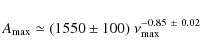
where
Using several 3D simulations of the surface of main-sequence stars, Samadi et al. (2007) have found that the maximum of the mode amplitude in velocity scales as (L/M)s with s=0.7.
This scaling law reproduces rather well the main-sequence stars
observed in Doppler velocity. When extrapolated to the red-giant domain
(
![]() ),
this scaling law illustrates a good agreement with the giant and
subgiant stars observed in Doppler velocity.
To derive the mode amplitude in terms of bolometric intensity
fluctuations from the mode amplitude in velocity, one usually assumes
the adiabatic relation proposed by Kjeldsen & Bedding (1995). For the mode amplitudes in intensity, this gives a scaling law of the form
),
this scaling law illustrates a good agreement with the giant and
subgiant stars observed in Doppler velocity.
To derive the mode amplitude in terms of bolometric intensity
fluctuations from the mode amplitude in velocity, one usually assumes
the adiabatic relation proposed by Kjeldsen & Bedding (1995). For the mode amplitudes in intensity, this gives a scaling law of the form
![]() ,
which requires the measurement of effective temperatures. Because of the Stefan-Boltzmann law, L/M scales as
,
which requires the measurement of effective temperatures. Because of the Stefan-Boltzmann law, L/M scales as
![]() ,
hence as
,
hence as
![]() .
.
As a consequence of Eq. (6),
![]() does not scale exactly as
does not scale exactly as
![]() .
We then obtain the scaling of the amplitude with
(L/M)s T-1/2 (Fig. 9)
.
We then obtain the scaling of the amplitude with
(L/M)s T-1/2 (Fig. 9)
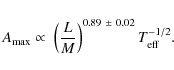
The spread around the global fit is as large as for the relation
![\begin{figure}
\par\includegraphics[width=8cm,clip]{14036fg10.ps}
\end{figure}](/articles/aa/full_html/2010/09/aa14036-10/img98.png)
|
Figure 10:
|
| Open with DEXTER | |
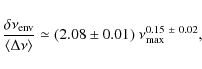
4.4 Height-to-background ratio
Owing to the large variety of stellar activity within the red-giant data set, the ratio
![]() does not obey a tight relation, but increases as
does not obey a tight relation, but increases as
![]() decreases (Fig. 10). By using the same method as for the amplitude, we derived the relation
decreases (Fig. 10). By using the same method as for the amplitude, we derived the relation
![]() .
This indicates first that it is possible to measure oscillation with a
large height-to-background ratio at very low frequency, which is
encouraging for future very long observations as will be provided by
Kepler.
.
This indicates first that it is possible to measure oscillation with a
large height-to-background ratio at very low frequency, which is
encouraging for future very long observations as will be provided by
Kepler.
The comparison of the mode amplitude and the
height-to-background ratio with frequency shows that the mean amplitude
of granulation and activity scales as
![]() .
This can be compared to Eq. (7)
with an exponent of about -0.85. If we link the amplitude to the
fraction of the convective energy injected in the oscillation, we
conclude that this fraction is greater at low frequency. Furthermore,
even if less convective energy is injected into the oscillation than
into granulation, the fraction injected in the oscillation increases
more rapidly at low frequency than the fraction injected into the
granulation.
.
This can be compared to Eq. (7)
with an exponent of about -0.85. If we link the amplitude to the
fraction of the convective energy injected in the oscillation, we
conclude that this fraction is greater at low frequency. Furthermore,
even if less convective energy is injected into the oscillation than
into granulation, the fraction injected in the oscillation increases
more rapidly at low frequency than the fraction injected into the
granulation.
![\begin{figure}
\par\includegraphics[width=8cm,clip]{14036fg11.ps}
\end{figure}](/articles/aa/full_html/2010/09/aa14036-10/img101.png)
|
Figure 11:
|
| Open with DEXTER | |
![\begin{figure}
\par\includegraphics[width=8cm,clip]{14036fg12a.ps}\par\vspace*{1mm}
\includegraphics[width=8cm,clip]{14036fg12b.ps}
\end{figure}](/articles/aa/full_html/2010/09/aa14036-10/img102.png)
|
Figure 12:
|
| Open with DEXTER | |
Table 4:
Scaling with
![]() .
.
5 Red-giant mass and radius estimate
It is possible to derive the stellar mass and radius from
![]() and
and
![]() ,
as done for example by Kallinger et al. (2010) for a few giant targets. This scaling assumes that the mean large separation
,
as done for example by Kallinger et al. (2010) for a few giant targets. This scaling assumes that the mean large separation
![]() is proportional to the mean stellar density and that
is proportional to the mean stellar density and that
![]() varies linearly with the cutoff frequency
varies linearly with the cutoff frequency
![]() ,
hence with
,
hence with
![]() ,
where g is the surface gravity (Brown et al. 1991). The analysis is extended here to a much larger set of targets, and measurements of higher quality than in Kallinger et al. (2010) because we have introduced the individual stellar effective temperatures.
,
where g is the surface gravity (Brown et al. 1991). The analysis is extended here to a much larger set of targets, and measurements of higher quality than in Kallinger et al. (2010) because we have introduced the individual stellar effective temperatures.
Before any measurements, we calibrated the scaling relations
given below, which provide the stellar mass and radius as a function of
the asteroseismic parameters, by comparing the seismic and modeled mass
and radius of red giants with already observed solar-like oscillations
(Table 3)
According to the targets summarized in Table 3, the factors r and m are
The equation that indicates the mass is highly degenerate, since
![]() is nearly constant according to Eq. (3).
This degeneracy shows that the temperature strongly impacts the stellar
mass. It also indicates that the dispersion about the scaling relation
(Eq. (3)) is the signature of the mass dispersion.
is nearly constant according to Eq. (3).
This degeneracy shows that the temperature strongly impacts the stellar
mass. It also indicates that the dispersion about the scaling relation
(Eq. (3)) is the signature of the mass dispersion.
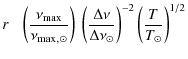
From Fig. 12, we derive the relation between the stellar radius and
![]() :
:

As in previous similar equations,
We analyzed this result to examine the extent to which the exponent
close to -1/2 is caused by the dependence of the cutoff frequency on
the gravity field g and to establish the relation between
![]() and
and
![]() .
To perform both steps in detail and to understand the difference reported in Eq. (3) relative to Stello et al. (2009), we assumed a variation in the cutoff frequency with
.
To perform both steps in detail and to understand the difference reported in Eq. (3) relative to Stello et al. (2009), we assumed a variation in the cutoff frequency with
![]() of
of
![]() ,
and then reapplied Eqs. (9) and (10), taking into account the scalings
,
and then reapplied Eqs. (9) and (10), taking into account the scalings
![]() and
and
![]() .
We obtained a new relation
.
We obtained a new relation
![]()

which has to be consistent with (Eq. (11)). Then, when we introduce the numerical values found for the exponents of the different fits, the comparison of Eq. (12) with Eq. (11) gives an exponent
From Table 1 of Kallinger et al. (2010) completed with a few other solar-targets benefitting from a precise modeling (HD 203608, Mosser et al. 2008; ![]() Hor, Teixeira et al. 2009; HD 52265, Ballot et al., in preparation; HD 170987, Mathur et al. 2010a; HD 46375, Gaulme et al. 2010), we can derive the exponent
Hor, Teixeira et al. 2009; HD 52265, Ballot et al., in preparation; HD 170987, Mathur et al. 2010a; HD 46375, Gaulme et al. 2010), we can derive the exponent ![]() from the values of
from the values of ![]() ,
,
![]() ,
and
,
and ![]() for main-sequence stars and for subgiants. In spite of the quite different set of exponents, we infer in both cases
for main-sequence stars and for subgiants. In spite of the quite different set of exponents, we infer in both cases
![]() ,
namely a relation between
,
namely a relation between
![]() and
and
![]() very close to linear (Table 4).
This proves that for all stellar classes the assumption of a fixed ratio
very close to linear (Table 4).
This proves that for all stellar classes the assumption of a fixed ratio
![]() is correct. Error bars for subgiants and main-sequence stars are larger
than in the red-giant case because of the limited set of stars, and
maybe also due to inhomogeneous modeling.
is correct. Error bars for subgiants and main-sequence stars are larger
than in the red-giant case because of the limited set of stars, and
maybe also due to inhomogeneous modeling.
![\begin{figure}
\par\includegraphics[width=8cm,clip]{14036fg13a.ps}\par\vspace*{1mm}
\includegraphics[width=8cm,clip]{14036fg13b.ps}
\end{figure}](/articles/aa/full_html/2010/09/aa14036-10/img132.png)
|
Figure 13: Histograms of the
stellar mass and radius. The curves in dark and light blue correspond,
respectively, to the components of the red clump around 30 and 40 |
| Open with DEXTER | |
![\begin{figure}
\par\includegraphics[width=8cm,clip]{14036fg14.ps}
\end{figure}](/articles/aa/full_html/2010/09/aa14036-10/img133.png)
|
Figure 14:
|
| Open with DEXTER | |
6 Red-giant population
6.1 Red clump
Miglio et al. (2009) compared synthetic, composite stellar populations to CoRoT observations. The analysis of the distribution in
![]() and
and
![]() allows them to identify red-clump giants and to estimate the properties
of poorly-constrained populations. Benefitting from both the reduction
in the error bars and the extension of the analysis to lower
frequencies compared to previous works, we can derive precise
properties of the red clump (Fig. 14).
allows them to identify red-clump giants and to estimate the properties
of poorly-constrained populations. Benefitting from both the reduction
in the error bars and the extension of the analysis to lower
frequencies compared to previous works, we can derive precise
properties of the red clump (Fig. 14).
The distribution of
![]() is centered around 30.2
is centered around 30.2 ![]() Hz with 69% of the values being within the range
Hz with 69% of the values being within the range
![]()
![]() Hz. The maximum of the distribution of
Hz. The maximum of the distribution of
![]() is located at
is located at
![]()
![]() Hz. The corresponding distribution of
Hz. The corresponding distribution of
![]() is centered around 3.96
is centered around 3.96 ![]() Hz with 69% of the values being within the range
Hz with 69% of the values being within the range
![]()
![]() Hz, and its maximum being located at
Hz, and its maximum being located at
![]()
![]() Hz. A second contribution of the red clump can be identified around 40
Hz. A second contribution of the red clump can be identified around 40 ![]() Hz. This feature may correspond to the secondary clump of red-giant stars predicted by Girardi (1999).
Hz. This feature may correspond to the secondary clump of red-giant stars predicted by Girardi (1999).
Table 5 presents the
mean values and the distribution of the physical parameters identified
for the peak and the shoulder of the clump stars: the mean values of
the radius are comparable for the two components, but the effective
temperature, mass, and luminosity are slightly different. The members
of the second component are hotter by about 80 K, brighter, and
significantly more massive. The mass distribution disagrees with the
theoretical prediction. The distribution is centered on 1.32 ![]() (Fig. 13), whereas Girardi (1999) predicts
(Fig. 13), whereas Girardi (1999) predicts
![]() for solar metallicity. Stars also appear to be brighter, in contrast to theoretical expectations. Figure 14 presents a zoom into the red-clump region of the
for solar metallicity. Stars also appear to be brighter, in contrast to theoretical expectations. Figure 14 presents a zoom into the red-clump region of the
![]() versus
versus
![]() relation and shows that stars less massive than
relation and shows that stars less massive than ![]() are numerous in the main component of the clump but rare in the shoulder. In constrast to Girardi (1999), we do not identify many stars with a mass above 2
are numerous in the main component of the clump but rare in the shoulder. In constrast to Girardi (1999), we do not identify many stars with a mass above 2 ![]() near the second component of the clump.
Selecting stars in the secondary component of the clump by adopting only a criterion on
near the second component of the clump.
Selecting stars in the secondary component of the clump by adopting only a criterion on
![]() is certainly insufficient, since many stars with
is certainly insufficient, since many stars with
![]() around 40
around 40 ![]() Hz can belong to the tail of the distribution of the main component. The discrepancy with the prediction of Girardi (1999)
may result from the way that we identify the stars and a refined
identification will be necessary to describe this secondary component
more accurately.
Hz can belong to the tail of the distribution of the main component. The discrepancy with the prediction of Girardi (1999)
may result from the way that we identify the stars and a refined
identification will be necessary to describe this secondary component
more accurately.
Table 5: Distribution of the red-clump parameters.
Figure 15 presents an HR diagram of the red-clump stars among all targets with precise asteroseismic parameters, the stellar luminosity being derived from the Stefan-Boltzmann law. We note a mass gradient in the direction of hot and luminous objects. However, we note that the members of the two components are intricately mixed in this diagram.
![\begin{figure}
\par\includegraphics[width=10.8cm,clip]{14036fg15.ps}
\vspace*{-1mm}
\end{figure}](/articles/aa/full_html/2010/09/aa14036-10/img168.png)
|
Figure 15:
HR diagram of the
|
| Open with DEXTER | |
6.2 Comparison center/anticenter
We compared the distribution of
![]() and
and
![]() in the 2 CoRoT runs LRc01 and LRa01. The LRc01 run, centered on
in the 2 CoRoT runs LRc01 and LRa01. The LRc01 run, centered on
![]() = (19h25min, 0
= (19h25min, 0![]() 30
30![]() ), targets an inner region of the Galaxy of Galactic longitude and latitude 37
), targets an inner region of the Galaxy of Galactic longitude and latitude 37![]() and
and ![]() 45
45![]() ,
respectively, 38
,
respectively, 38![]() away from the Galactic center.
Targets of the run LRa01 are located in the opposite direction of LRc01, centered on
away from the Galactic center.
Targets of the run LRa01 are located in the opposite direction of LRc01, centered on
![]() = (6h42min,
= (6h42min, ![]() 30
30![]() ), of lower Galactic latitude (
), of lower Galactic latitude (![]() 45
45![]() )
and Galactic longitude of 212
)
and Galactic longitude of 212![]() .
According to the reddening inferred for the targets, a typical 13th
magnitude red giant of the red clump is located at 3 kpc.
.
According to the reddening inferred for the targets, a typical 13th
magnitude red giant of the red clump is located at 3 kpc.
The histograms of
![]() and
and
![]() for both fields are compared in Fig. 16.
They show comparable relative values in all frequency ranges except for
the location of the clump stars. The main component of the red clump is
much less pronounced in LRa01 than LRc01; on the other hand, the second
component of the clump is more populated in LRa01. The distribution
concerning LRa01, with two components, strongly supports the
identification of the secondary clump.
Since the two populations were selected on the basis of homogeneous
criteria and show comparable scaling laws for all asteroseismic
parameters, understanding the difference between them will require
additional analysis taking into account more parameters than those
given by asteroseismology, to investigate the roles of evolutionary
status, metallicity, and position in the Galaxy.
for both fields are compared in Fig. 16.
They show comparable relative values in all frequency ranges except for
the location of the clump stars. The main component of the red clump is
much less pronounced in LRa01 than LRc01; on the other hand, the second
component of the clump is more populated in LRa01. The distribution
concerning LRa01, with two components, strongly supports the
identification of the secondary clump.
Since the two populations were selected on the basis of homogeneous
criteria and show comparable scaling laws for all asteroseismic
parameters, understanding the difference between them will require
additional analysis taking into account more parameters than those
given by asteroseismology, to investigate the roles of evolutionary
status, metallicity, and position in the Galaxy.
![\begin{figure}
\par\includegraphics[width=7.8cm,clip]{14036fg16a.ps}\par\vspace*{1mm}
\includegraphics[width=7.8cm,clip]{14036fg16b.ps}\vspace*{-2mm}
\end{figure}](/articles/aa/full_html/2010/09/aa14036-10/img175.png)
|
Figure 16:
Histograms of
|
| Open with DEXTER | |
7 Conclusion
We have demonstrated that it is possible to extract statistical information from the high-precision photometric time series of a large sample of red giants observed with CoRoT and analyzed with an automated asteroseismic pipeline. We summarize here the main results of our study and the remaining open issues:
- Out of more than 4600 time series, we have identified more than 1800 red giants exhibiting solar-like oscillations. We have extracted a full set of precise asteroseismic parameters for more than 900 targets.
- Thanks to our detection method, we have been able to observe precisely large separations as small as 0.75
 Hz. We have obtained reliable information about the seismic parameters
 and
and
 for
in the range [3.5, 100 Hz]. We have shown that the detection and measurement method does not introduce any bias for
above 6 Hz. This allows us to study in detail the red clump in the range [30, 40 Hz].
for
in the range [3.5, 100 Hz]. We have shown that the detection and measurement method does not introduce any bias for
above 6 Hz. This allows us to study in detail the red clump in the range [30, 40 Hz].
- We have proposed scaling relations for the parameters defining
the envelope where the asteroseismic power is observed in excess. We
note that the relation defining the full-width at half-maximum
 of the envelope cannot be extended to solar-like stars. The scaling relation between
and
is definitely not linear for giants, being
of the envelope cannot be extended to solar-like stars. The scaling relation between
and
is definitely not linear for giants, being
 .
The maximum amplitude scales as
.
The maximum amplitude scales as
 or
(L/M)0.89.
Deriving bolometric amplitudes will require more work, including
examination of the equipartition of energy between the modes and
stellar atmosphere modeling.
or
(L/M)0.89.
Deriving bolometric amplitudes will require more work, including
examination of the equipartition of energy between the modes and
stellar atmosphere modeling.
- When complemented with effective temperature, asteroseismic parameters
and
can
be used to determine the stellar mass and radius. Red-giant masses
derived from asteroseismology are degenerate, but their value can be
estimated with a typical uncertainty of about 20%.
We have established a tight relation between the maximum amplitude
frequency
and the red-giant radius from an unbiased analysis in the range [
 ], which encompasses the red-clump stars. This relation scales as
 .
.
- From this result, and taking into account the scaling law
 ,
we have shown that the ratio
,
we have shown that the ratio
 is constant for giants. A similar analysis performed on main-sequence stars and subgiants reaches the same result:
is also nearly constant.
is constant for giants. A similar analysis performed on main-sequence stars and subgiants reaches the same result:
is also nearly constant.
- As a by-product, we have shown that scaling laws are slightly but undoubtedly different for giants, subgiants and dwarfs. For red-giant stars only, that the temperature is nearly a degenerate parameter plays a significant role. As a consequence, global fits encompassing all stars with solar-like oscillations may not be precise, since they do not account for the different physical conditions between main-sequence and giant stars.
- The comparison of data from 2 runs pointing in different directions at different Galactic latitudes has shown that the stellar properties are similar; the dispersion about the global fits is too small to be detectable. The main difference between the 2 runs is their different stellar populations. The distributions of the asteroseismic parameters are globally similar, except for the location of the red clump.
- We have obtained precise information about the red-clump stars. Statistical asteroseismology makes it possible to identify the expected secondary clump and to measure the distribution of the fundamental parameters of the red-clump stars. We have shown that the relative importance of the two components of the clump is linked to the stellar population. The precise determination of the red-clump parameters will benefit from the asteroseismic analysis and the modeling of individual members of the clump.
This work was supported by the Centre National d'Études Spatiales (CNES). It is based on observations with CoRoT. The research has made use of the Exo-Dat database, operated at LAM-OAMP, Marseille, France, on behalf of the CoRoT/Exoplanet program. TM acknowledges financial support from Belspo for contract PRODEX-GAIA DPAC.The work of K.B. was supported through a postdoctoral fellowship from the ``Subside fédéral pour la recherche 2010'', Université de Liège. S.H. acknowledges support by the UK Science and Technology Facilities Council. The research leading to these results has received funding from the European Research Council under the European Community's Seventh Framework Programme (FP7/2007-2013)/ERC grant agreement n
227224 (PROSPERITY), as well as from the Research Council of K.U.Leuven grant agreement GOA/2008/04.
References
- Alonso, A., Arribas, S., & Martínez-Roger, C. 1999, A&AS, 140, 261 [NASA ADS] [CrossRef] [EDP Sciences] [Google Scholar]
- Appourchaux, T. 2004, A&A, 428, 1039 [NASA ADS] [CrossRef] [EDP Sciences] [Google Scholar]
- Appourchaux, T., Michel, E., Auvergne, M., et al. 2008, A&A, 488, 705 [NASA ADS] [CrossRef] [EDP Sciences] [Google Scholar]
- Auvergne, M., Bodin, P., Boisnard, L., et al. 2009, A&A, 506, 411 [NASA ADS] [CrossRef] [EDP Sciences] [Google Scholar]
- Barban, C., De Ridder, J., Mazumdar, A., et al. 2004, in SOHO 14 Helio- and Asteroseismology: Towards a Golden Future, ed. D. Danesy, ESA SP, 559, 113 [Google Scholar]
- Barban, C., Matthews, J. M., De Ridder, J., et al. 2007, A&A, 468, 1033 [NASA ADS] [CrossRef] [EDP Sciences] [Google Scholar]
- Barban, C., Deheuvels, S., Baudin, F., et al. 2009, A&A, 506, 51 [NASA ADS] [CrossRef] [EDP Sciences] [Google Scholar]
- Baudin, F., Barban, C., Belkacem, K., et al. 2010, A&A, submitted [Google Scholar]
- Bedding, T., Huber, D., Stello, D., et al. 2010, ApJ, 713, L176 [NASA ADS] [CrossRef] [Google Scholar]
- Benomar, O., Baudin, F., Campante, T. L., et al. 2009, A&A, 507, L13 [NASA ADS] [CrossRef] [EDP Sciences] [Google Scholar]
- Brown, T. M., Gilliland, R. L., Noyes, R. W., & Ramsey, L. W. 1991, ApJ, 368, 599 [NASA ADS] [CrossRef] [Google Scholar]
- Carrier, F., De Ridder, J., Baudin, F., et al. 2010, A&A, 509, A73 [NASA ADS] [CrossRef] [EDP Sciences] [Google Scholar]
- De Ridder, J., Barban, C., Baudin, F., et al. 2009, Nature, 459, 398 [Google Scholar]
- Deheuvels, S., Bruntt, H., Michel, E., et al. 2010, A&A, 515, A87 [NASA ADS] [CrossRef] [EDP Sciences] [Google Scholar]
- Deleuil, M., Meunier, J. C., Moutou, C., et al. 2009, AJ, 138, 649 [NASA ADS] [CrossRef] [Google Scholar]
- Dobashi, K., Uehara, H., Kandori, R., et al. 2005, PASJ, 57, S1 [NASA ADS] [CrossRef] [Google Scholar]
- Dupret, M., Belkacem, K., Samadi, R., et al. 2009, A&A, 506, 57 [NASA ADS] [CrossRef] [EDP Sciences] [Google Scholar]
- Frandsen, S., Carrier, F., Aerts, C., et al. 2002, A&A, 394, L5 [NASA ADS] [CrossRef] [EDP Sciences] [Google Scholar]
- García, R. A., Régulo, C., Samadi, R., et al. 2009, A&A, 506, 41 [NASA ADS] [CrossRef] [EDP Sciences] [Google Scholar]
- Gaulme, P., Deheuvels, S., Weiss, W. W., et al. 2010, A&A, submitted [Google Scholar]
- Girardi, L. 1999, MNRAS, 308, 818 [NASA ADS] [CrossRef] [MathSciNet] [Google Scholar]
- Hekker, S., Aerts, C., De Ridder, J., & Carrier, F. 2006, A&A, 458, 931 [NASA ADS] [CrossRef] [EDP Sciences] [Google Scholar]
- Hekker, S., Kallinger, T., Baudin, F., et al. 2009, A&A, 506, 465 [NASA ADS] [CrossRef] [EDP Sciences] [Google Scholar]
- Huber, D., Stello, D., Bedding, T. R., et al. 2009, Commun. Asteroseismol., 160, 74 [NASA ADS] [CrossRef] [Google Scholar]
- Kallinger, T., Guenther, D. B., Matthews, J. M., et al. 2008, A&A, 478, 497 [NASA ADS] [CrossRef] [EDP Sciences] [Google Scholar]
- Kallinger, T., Weiss, W. W., Barban, C., et al. 2010, A&A, 509, A77 [NASA ADS] [CrossRef] [EDP Sciences] [Google Scholar]
- Kjeldsen, H., & Bedding, T. R. 1995, A&A, 293, 87 [NASA ADS] [Google Scholar]
- Mathur, S., Garcia, R., Catala, C., et al. 2010a, A&A, accepted [Google Scholar]
- Mathur, S., García, R. A., Régulo, C., et al. 2010b, A&A, 511, A46 [NASA ADS] [CrossRef] [EDP Sciences] [Google Scholar]
- Mazumdar, A., Mérand, A., Demarque, P., et al. 2009, A&A, 503, 521 [NASA ADS] [CrossRef] [EDP Sciences] [Google Scholar]
- Michel, E., Samadi, R., Baudin, F., et al. 2009, A&A, 495, 979 [NASA ADS] [CrossRef] [EDP Sciences] [Google Scholar]
- Miglio, A., Montalbán, J., Baudin, F., et al. 2009, A&A, 503, L21 [NASA ADS] [CrossRef] [EDP Sciences] [MathSciNet] [Google Scholar]
- Mosser, B., & Appourchaux, T. 2009, A&A, 508, 877 [NASA ADS] [CrossRef] [EDP Sciences] [Google Scholar]
- Mosser, B., & Appourchaux, T. 2010, in New insights into the Sun, ed. M. Cunha, & M. Monteiro, in press [Google Scholar]
- Mosser, B., Bouchy, F., Catala, C., et al. 2005, A&A, 431, L13 [NASA ADS] [CrossRef] [EDP Sciences] [Google Scholar]
- Mosser, B., Deheuvels, S., Michel, E., et al. 2008, A&A, 488, 635 [NASA ADS] [CrossRef] [EDP Sciences] [Google Scholar]
- Mosser, B., Michel, E., Appourchaux, T., et al. 2009, A&A, 506, 33 [NASA ADS] [CrossRef] [EDP Sciences] [Google Scholar]
- Rowles, J., & Froebrich, D. 2009, MNRAS, 395, 1640 [NASA ADS] [CrossRef] [Google Scholar]
- Roxburgh, I. W., & Vorontsov, S. V. 2006, MNRAS, 369, 1491 [NASA ADS] [CrossRef] [Google Scholar]
- Samadi, R., Georgobiani, D., Trampedach, R., et al. 2007, A&A, 463, 297 [NASA ADS] [CrossRef] [EDP Sciences] [Google Scholar]
- Stello, D., Chaplin, W. J., Basu, S., Elsworth, Y., & Bedding, T. R. 2009, MNRAS, 400, L80 [NASA ADS] [CrossRef] [Google Scholar]
- Stello, D., Basu, S., Bruntt, H., Mosser, B., & Stevens, I. 2010, ApJ, 713, L182 [NASA ADS] [CrossRef] [Google Scholar]
- Teixeira, T. C., Kjeldsen, H., Bedding, T. R., et al. 2009, A&A, 494, 237 [NASA ADS] [CrossRef] [EDP Sciences] [Google Scholar]
Footnotes
- ... CoRoT
- The CoRoT space mission, launched on 2006 December 27, was developed and is operated by the CNES, with participation of the Science Programs of ESA, ESAs RSSD, Austria, Belgium, Brazil, Germany and Spain.
- ...2,
- Postdoctoral Researcher, Fonds de la Recherche Scientifique - FNRS, Belgium.
All Tables
Table 1: Red-giant targets.
Table 2: Number of detected peaks.
Table 3: Calibration of the red-giant mass and radius.
Table 4:
Scaling with
![]() .
.
Table 5: Distribution of the red-clump parameters.
All Figures
|
|
Figure 1:
Fourier spectrum of a target with a very low mean value of the large separation (
|
| Open with DEXTER | |
| In the text | |
|
|
Figure 2:
Estimation of the bias, calculated from the mean ratio
|
| Open with DEXTER | |
| In the text | |
|
|
Figure 3:
|
| Open with DEXTER | |
| In the text | |
|
|
Figure 4:
Histogram of
|
| Open with DEXTER | |
| In the text | |
|
|
Figure 5:
Histogram of
|
| Open with DEXTER | |
| In the text | |
|
|
Figure 6:
|
| Open with DEXTER | |
| In the text | |
|
|
Figure 7:
|
| Open with DEXTER | |
| In the text | |
|
|
Figure 8:
|
| Open with DEXTER | |
| In the text | |
|
|
Figure 9:
|
| Open with DEXTER | |
| In the text | |
|
|
Figure 10:
|
| Open with DEXTER | |
| In the text | |
|
|
Figure 11:
|
| Open with DEXTER | |
| In the text | |
|
|
Figure 12:
|
| Open with DEXTER | |
| In the text | |
|
|
Figure 13: Histograms of the
stellar mass and radius. The curves in dark and light blue correspond,
respectively, to the components of the red clump around 30 and 40 |
| Open with DEXTER | |
| In the text | |
|
|
Figure 14:
|
| Open with DEXTER | |
| In the text | |
|
|
Figure 15:
HR diagram of the
|
| Open with DEXTER | |
| In the text | |
|
|
Figure 16:
Histograms of
|
| Open with DEXTER | |
| In the text | |
Copyright ESO 2010
Current usage metrics show cumulative count of Article Views (full-text article views including HTML views, PDF and ePub downloads, according to the available data) and Abstracts Views on Vision4Press platform.
Data correspond to usage on the plateform after 2015. The current usage metrics is available 48-96 hours after online publication and is updated daily on week days.
Initial download of the metrics may take a while.