| Issue |
A&A
Volume 517, July 2010
|
|
|---|---|---|
| Article Number | A25 | |
| Number of page(s) | 7 | |
| Section | Cosmology (including clusters of galaxies) | |
| DOI | https://doi.org/10.1051/0004-6361/200913977 | |
| Published online | 28 July 2010 | |
A search for edge-on galaxy lenses in the CFHT Legacy Survey![[*]](/icons/foot_motif.png)
J. F. Sygnet1,2 - H. Tu3,1,2 - B. Fort1,2 - R. Gavazzi1,2
1 - CNRS, UMR7095, Institut d'Astrophysique de Paris, 75014 Paris, France
2 -
UPMC Univ Paris 06, UMR7095, Institut d'Astrophysique de Paris, 75014 Paris, France
3 -
Physics Department & Shanghai Key Lab for Astrophysics, Shanghai Normal University, Shanghai 200234, PR China
Received 28 December 2009 / Accepted 18 April 2010
Abstract
Context. The new generation of wide-field optical imaging as
the Canada France Hawaii Telescope Legacy Survey (CFHTLS) enables
discoveries of all types of gravitational lenses present in the sky.
The Strong Lensing Legacy Survey (SL2S) project has started an
inventory of clusters or groups of galaxies lenses and of Einstein
rings around distant massive ellipticals.
Aims. Here we attempt to extend this inventory by finding
lensing events produced by massive edge-on disk galaxies that remain a
poorly documented class of lenses.
Methods. We implemented and tested an automated search procedure
of edge-on galaxy lenses in the CFHTLS Wide fields with magnitude 18<i<21, inclination angle lower than
![]() ,
and a photometric redshift determination. This procedure estimated the
lensing convergence of each galaxy from the Tully-Fisher law and
selected only those few candidates that exhibit a possibly nearby arc
configuration at a radius compatible with this convergence (
,
and a photometric redshift determination. This procedure estimated the
lensing convergence of each galaxy from the Tully-Fisher law and
selected only those few candidates that exhibit a possibly nearby arc
configuration at a radius compatible with this convergence (
![]() ).
The efficiency of the procedure was tested after a visual examination
of the whole initial sample of 30 444 individual edge-on disks.
).
The efficiency of the procedure was tested after a visual examination
of the whole initial sample of 30 444 individual edge-on disks.
Results. After calculating the surface density of edge-on lenses
possibly detected in a survey for a given seeing, we deduce that this
theoretical number is about 10 for the CFHTLS Wide, a number in broad
agreement with the 2 good candidates detected here. We show that the
Tully-Fisher selection method is very efficient at finding valuable
candidates, though its accuracy depends on the quality of the
photometric redshift of the lenses. Finally, we argue that future
surveys will detect at least a hundred of such lens candidates.
Key words: gravitational lensing: strong - dark matter - galaxies: spiral - galaxies: halos
1 Introduction
The ![]() -CDM cosmological paradigm has been highly successful at explaining most
of the large-scale properties of the Universe; nevertheless it still must be shown
that this model is able to explain its small-scale properties.
Among these are the formation and dark matter content of disk galaxies, and in
particular the rotation curves of disks have played a key role as evidence
that there is dark matter on small scales
(e.g. Rubin et al. 1980; de Blok et al. 2008; Bosma 1978; Donato et al. 2009; Persic et al. 1996).
Despite tremendous observational and modeling efforts over the past three decades,
advances are still plagued by our ability to disentangle both
the contributions of baryonic disk and bulges and the contribution of dark matter.
-CDM cosmological paradigm has been highly successful at explaining most
of the large-scale properties of the Universe; nevertheless it still must be shown
that this model is able to explain its small-scale properties.
Among these are the formation and dark matter content of disk galaxies, and in
particular the rotation curves of disks have played a key role as evidence
that there is dark matter on small scales
(e.g. Rubin et al. 1980; de Blok et al. 2008; Bosma 1978; Donato et al. 2009; Persic et al. 1996).
Despite tremendous observational and modeling efforts over the past three decades,
advances are still plagued by our ability to disentangle both
the contributions of baryonic disk and bulges and the contribution of dark matter.
The hypothesis of the maximum bulge or disk (van Albada & Sancisi 1986; Dutton et al. 2005; Persic et al. 1996) is able to fix the mass-to-light ratio of the stellar populations and therefore to put constraints on the dark matter content of galaxies or, alternatively, on inferences about modifications of the gravitation law (e.g. McGaugh 2004; de Blok et al. 2008; de Blok & McGaugh 1997; Donato et al. 2009). For further insight into the relative contribution of different species (stars in disk, stars in bulge, and dark matter), one needs additional constraints to break the degeneracies (e.g. Ibata et al. 2007; Kranz et al. 2003; de Jong & Bell 2007).
Another particularly promising method resides in studying the dynamical properties of strong lensing galaxies. Mostly because of the scarcity of background QSOs, only very few lensing disk galaxies with a low enough redshift, suitable for kinematical observations, have been known until recently. For instance, one can mention the early studies of the Einstein Cross Q2237-0305 (Trott & Webster 2002; Trott et al. 2010; van de Ven et al. 2008), of B1600+434 (Jaunsen & Hjorth 1997; Koopmans et al. 1998; Maller et al. 2000), of J2004-1349 (Winn et al. 2003), of CXOCY J220132.8-320144 (Castander et al. 2006), or Q0045-3337 (Chieregato et al. 2007).
Great advances have become possible recently thanks to the advent of
large high-quality imaging and spectroscopic datasets.
Automated or visual inspection of high-resolution imaging from the
Hubble Space Telescope (HST) (e.g. Faure et al. 2008; Moustakas et al. 2007; Covone et al. 2009; Newton et al. 2009; Marshall et al. 2009) or from the ground
(e.g. Cabanac et al. 2007; Kubo & Dell'Antonio 2008)
have just started to provide us with many candidates for strong galaxy-galaxy lensing events.
For spectroscopy, an automated search of superimposed spectra at different redshifts
into a given fiber followed up by high-resolution HST imaging turns out to be very
efficient on large spectroscopic datasets like the Sloan Digital Sky Survey (SDSS) (Bolton et al. 2004; Willis et al. 2006,2005; Bolton et al. 2008; Auger et al. 2009; Bolton et al. 2006).
These studies are limited to relatively low redshifts (![]() ), and most of
them focus on lensing by massive elliptical galaxies with a large splitting angle.
), and most of
them focus on lensing by massive elliptical galaxies with a large splitting angle.
Conversely, late-type galaxies, while more numerous
(e.g. Kochanek 2006; Bartelmann 2000; Chae 2010),
have a smaller Einstein radius and are thus more difficult to identify.
For instance the recently found edge-on disk galaxy OAC-GL J1223-1239
(Covone et al. 2009), with
![]() ,
could only be found
with HST imaging.
A first automated spectroscopic search for disk galaxies lenses in
the SDSS database was done by Féron et al. (2009):
they found 8 candidates among 40 000 disk galaxies, two of them being
already confirmed as genuine lenses.
,
could only be found
with HST imaging.
A first automated spectroscopic search for disk galaxies lenses in
the SDSS database was done by Féron et al. (2009):
they found 8 candidates among 40 000 disk galaxies, two of them being
already confirmed as genuine lenses.
Despite these efforts, disk galaxies remain a poorly documented class of lenses, particularly for edge-on lensing galaxies. This situation calls for an improvement. We need more edge-on disk lenses with a low inclination to maximize the success of dynamical studies and simplify the recognition of lensing/lensed structures in imaging data. In this paper we investigate if the deep multiband sub-arcsecond imaging data of the Canada France Hawaii Telescope Legacy Survey (CFHTLS) offers a good opportunity to find edge-on disk lenses beyond the redshift range accessible by the SDSS.
The paper is organized as follows.
Section 2 presents a calculation of the number of lenses
with an i magnitude
18 < i < 21 and an inclination lower than
![]() which should be detected for a given seeing in an imaging survey.
Section 3 explains the procedure that we have followed to
extract edge-on lens candidates from the CFHTLS Wide survey by estimating
an Einstein radius from the Tully-Fisher (TF) relation (Tully & Fisher 1977)
and comparing it with the arc radius possibly detected around the galaxy.
We also cross-check the validity of this automated procedure
by a visual inspection of all the edge-on galaxies present in the survey.
In Sect. 4 we discuss our results with an overview on what could
be done with future all-sky imaging surveys.
Throughout this paper all magnitudes are expressed in the AB system,
and we assume the concordance cosmological model with h = 0.7,
which should be detected for a given seeing in an imaging survey.
Section 3 explains the procedure that we have followed to
extract edge-on lens candidates from the CFHTLS Wide survey by estimating
an Einstein radius from the Tully-Fisher (TF) relation (Tully & Fisher 1977)
and comparing it with the arc radius possibly detected around the galaxy.
We also cross-check the validity of this automated procedure
by a visual inspection of all the edge-on galaxies present in the survey.
In Sect. 4 we discuss our results with an overview on what could
be done with future all-sky imaging surveys.
Throughout this paper all magnitudes are expressed in the AB system,
and we assume the concordance cosmological model with h = 0.7,
![]() ,
and
,
and
![]() .
.
2 Forecasting the frequency of edge-on disk lenses
We attempt here to predict the number of lenses that could be observed within an imaging survey of properties similar to the CFHTLS Wide.
2.1 Cross-sections and optical depths
We estimate lensing optical depths by starting from generic assumptions about mass
distributions (see e.g. Schneider et al. 1992; Turner et al. 1984; Kochanek 2006; Marshall et al. 2005).
In particular, we assume that all lenses are singular isothermal spheres
(SIS) parameterized by their velocity dispersion ![]() .
They are also assumed to be sparse enough that the probability of multiple
lensing is negligible, so that one can sum up individual lensing
cross-sections over the probed volume.
Arguably, circular symmetry might not be a good description of edge-on disk galaxies.
Bartelmann & Loeb (1998) showed that, averaging over all possible inclination
angles, the effect of the disk is null for the overall cross-section.
It is however found that the efficiency of edge-on lenses is a bit boosted
so that a calculation of the total SIS cross-section and the same calculation
restricted to inclinations
.
They are also assumed to be sparse enough that the probability of multiple
lensing is negligible, so that one can sum up individual lensing
cross-sections over the probed volume.
Arguably, circular symmetry might not be a good description of edge-on disk galaxies.
Bartelmann & Loeb (1998) showed that, averaging over all possible inclination
angles, the effect of the disk is null for the overall cross-section.
It is however found that the efficiency of edge-on lenses is a bit boosted
so that a calculation of the total SIS cross-section and the same calculation
restricted to inclinations
![]() (corresponding to a third
of all possible orientations) consistent with edge-on disks will bracket the
right number.
So we define a corrective term
(corresponding to a third
of all possible orientations) consistent with edge-on disks will bracket the
right number.
So we define a corrective term
![]() that will multiply the total lensing
cross-section of disky galaxies approximated as SIS.
that will multiply the total lensing
cross-section of disky galaxies approximated as SIS.
Ideally, the cross-section X for multiple imaging by an SIS mass distribution
at redshift ![]() of a source at
of a source at ![]() is given by the solid angle
(in steradians) subtended by the Einstein radius:
is given by the solid angle
(in steradians) subtended by the Einstein radius:
![\begin{displaymath}X= \pi r_{\rm E}^2 = \pi \left[ 4\pi \left( \frac{\sigma}{c}\right)^2
\frac{D_{\rm ls}}{D_{\rm os}}\right]^2\cdot
\end{displaymath}](/articles/aa/full_html/2010/09/aa13977-09/img15.png)
|
(1) |
However, due to observational limitations, one cannot detect all the lenses of a given
|
(2) |
The optical depth
In this equation we have introduced a selection function
![\begin{displaymath}\phi(\sigma) = \phi^* \sigma^{-1} \left( \frac{\sigma}{\sigma...
...}\right)^\beta\right]
\frac{\beta}{\Gamma (\alpha / \beta)} ,
\end{displaymath}](/articles/aa/full_html/2010/09/aa13977-09/img35.png)
|
(4) |
with
2.2 Selection function of lenses
As already anticipated, observational limitations will lead to a non-unity
selection function
![]() .
Obviously we cannot directly select on
.
Obviously we cannot directly select on ![]() or
or ![]() but, more realistically,
we use apparent magnitudes.
Therefore we assume that a combination of photometric redshifts (with negligible
errors at this stage) and a direct relation between luminosity and velocity
dispersion will approximate most of the observational selections effects.
More precisely, assuming that lens galaxies are isothermal spheres allows
us to relate the
velocity dispersion to the rotation velocity
but, more realistically,
we use apparent magnitudes.
Therefore we assume that a combination of photometric redshifts (with negligible
errors at this stage) and a direct relation between luminosity and velocity
dispersion will approximate most of the observational selections effects.
More precisely, assuming that lens galaxies are isothermal spheres allows
us to relate the
velocity dispersion to the rotation velocity
![]() .
We then use the latest normalization of the Tully-Fischer relation in the R band
from Pizagno et al. (2007) and neglect the intrinsic scatter about
the mean relation, giving
.
We then use the latest normalization of the Tully-Fischer relation in the R band
from Pizagno et al. (2007) and neglect the intrinsic scatter about
the mean relation, giving
|
(5) |
In addition, we shift apparent i band magnitudes back to the rest frame r band using a redshift dependent k-correction so that
|
(6) |
which is obtained by redshifting template of Sbc galaxies from Coleman et al. (1980) using hyperz facility (Bolzonella et al. 2000). Hence a given selection in magnitude
2.3 Population of background sources
Given the lensing optical depth of Eq. (3) and a redshift
distribution of sources, the number of lenses can be written as
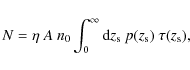
|
(7) |
where A is the surveyed area and
with z0=0.345 and a=3.89 (Gavazzi et al. 2007). In addition, at these limiting i<26 magnitudes, one can achieve a surface density of sources of about
2.4 Results
For the values considered above, we plot in Fig. 1 the predicted
number of edge-on disks as a function of the cut radius which is identified
to the seeing.
For the CFHTLS Wide image quality (seeing
![]() in
g band) and depth we typically get about 0.07-0.30 detectable lenses per
square degree depending on the edge-on disk boost factor
in
g band) and depth we typically get about 0.07-0.30 detectable lenses per
square degree depending on the edge-on disk boost factor ![]() .
Therefore for the 124 deg2 imaged in five u*griz bands, one might discover
between 8 and 37 lenses assuming all our hypotheses (SIS density profile, no
scatter in the TF relation nor errors with photometric redshifts...) are correct.
.
Therefore for the 124 deg2 imaged in five u*griz bands, one might discover
between 8 and 37 lenses assuming all our hypotheses (SIS density profile, no
scatter in the TF relation nor errors with photometric redshifts...) are correct.
To assess our calculations we also made predictions for the number of lensing
elliptical galaxies assuming a perfect relation between magnitude and velocity
dispersion as given by the Faber-Jackson relation whose normalization is taken
from Oguri (2006).
Down to a limiting AB magnitude i<22.5 for the deflector, a similar
calculation based on the velocity dispersion function for ellipticals also
given by Chae (2010) yields the red curve in Fig. 1.
It predicts 10 to 100 more lenses with a substantially lower dependence
on seeing below
![]() .
This might be explained by the generally larger Einstein radius (due to greater
velocity dispersions) of ellipticals for which the exponential fall-off of
the distribution functions drops beyond
.
This might be explained by the generally larger Einstein radius (due to greater
velocity dispersions) of ellipticals for which the exponential fall-off of
the distribution functions drops beyond
![]() .
Worse seeing will also make
the detectability of arcs and counterimages much more challenging beyond
.
Worse seeing will also make
the detectability of arcs and counterimages much more challenging beyond
![]() .
In addition, the light from the deflector, no matter the seeing size, will
prevent many small-scale detections.
For comparison, Marshall et al. (2005) predicted about 50 lenses that could
be detected by SNAP (two magnitudes deeper with
.
In addition, the light from the deflector, no matter the seeing size, will
prevent many small-scale detections.
For comparison, Marshall et al. (2005) predicted about 50 lenses that could
be detected by SNAP (two magnitudes deeper with
![]() ).
Ten or so systems would remain by degrading depth and image quality to
our survey specifications and by restricting ourselves to bright i<22.5deflectors. This is consistent with our calculations.
This is also in broad agreement with COSMOS observations of strong
lensing luminous
Mr< -20 ellipticals (Faure et al. 2008).
).
Ten or so systems would remain by degrading depth and image quality to
our survey specifications and by restricting ourselves to bright i<22.5deflectors. This is consistent with our calculations.
This is also in broad agreement with COSMOS observations of strong
lensing luminous
Mr< -20 ellipticals (Faure et al. 2008).
![\begin{figure}
\includegraphics[width=9cm,clip]{13977fig1.eps}
\end{figure}](/articles/aa/full_html/2010/09/aa13977-09/img53.png)
|
Figure 1:
Predicted number of gravitational lenses per square degree as
a function of image quality.
Imaging survey specifications in terms of depth are those of the CFHTLS Wide.
The dashed and dot-dashed black lines bracket the number of lensing
edge-on disks depending on the edge-on disk boost factor |
| Open with DEXTER | |
3 Seeking edge-on disk lenses within the CFHTLS Wide
From the calculations above, we can undertake a comprehensive search of
lenses in the CFHTLS Wide survey.
The T0005 data release (for a detailed description, see Mellier et al. 2008)
spans 171 fields of one square degree each
for which images in at least the three g, r, and i bands are obtained.
But, in order to calculate the photometric ![]() of the possible lenses,
we restrict ourselves to the 124 fields for which the five u*, g, r,
i, and z bands are present.
The typical 80% completeness limit magnitude for point sources is
25.4, 25.4, 24.6, 24.5, and 23.6 respectively. Image quality is also
very good with typical seeing FWHM of
of the possible lenses,
we restrict ourselves to the 124 fields for which the five u*, g, r,
i, and z bands are present.
The typical 80% completeness limit magnitude for point sources is
25.4, 25.4, 24.6, 24.5, and 23.6 respectively. Image quality is also
very good with typical seeing FWHM of
![]() and
and
![]() respectively.
respectively.
3.1 Photometric preselection of bright edge-on galaxies
We start from a catalog of 28 million extended objects detected with SExtractor (Bertin & Arnouts 1996). We first select 1.02 million objects within the magnitude range 18 < i < 21as the initial data base. The bright i < 18 low redshift galaxies are excluded because their angular size is too large as compared to their expected Einstein radius. Objects fainter than i = 21 are also discarded because of the low signal-to-noise and the difficulty of future spectroscopic follow-up. The few already known spiral galaxies producing multiply-imaged QSOs happened to be in this magnitude range (Chieregato et al. 2007; Koopmans et al. 1998; Castander et al. 2006; Maller et al. 2000).
Edge-on disk galaxies are then preselected as highly elongated objects with
projected ellipticity
![]() .
The lower limit on the ellipticity is chosen because it removes most of
the ellipticals (Park et al. 2007) while the upper limit e<0.92 stands for
rejecting most (
.
The lower limit on the ellipticity is chosen because it removes most of
the ellipticals (Park et al. 2007) while the upper limit e<0.92 stands for
rejecting most (![]() 90%) of spurious objects like diffraction
patterns of bright stars.
This ellipticity cut yields 30 444 bright edge-on galaxies.
90%) of spurious objects like diffraction
patterns of bright stars.
This ellipticity cut yields 30 444 bright edge-on galaxies.
3.2 The Tully-Fischer relation as a proxy for Einstein radius
The multiband (u*griz) photometry of the survey allows the computation
of photometric redshifts (Coupon et al. 2009).
Along with apparent magnitudes, this additional information enables
estimates of absolute magnitudes that can readily be converted into an
estimate of their rotation velocity ![]() using the latest calibrations
of the Tully-Fischer relation (Pizagno et al. 2007).
Assuming the lensing galaxy can be approximated by a circularly symmetric
isothermal mass distribution, the velocity dispersion is
using the latest calibrations
of the Tully-Fischer relation (Pizagno et al. 2007).
Assuming the lensing galaxy can be approximated by a circularly symmetric
isothermal mass distribution, the velocity dispersion is
![]() .
Using a typical source redshift
.
Using a typical source redshift
![]() and taking into account
a possible error
and taking into account
a possible error
![]() on the absolute magnitude
(corresponding to the
on the absolute magnitude
(corresponding to the ![]() -dispersion of the TF law), we can predict
an Einstein radius
-dispersion of the TF law), we can predict
an Einstein radius
![]() that is then compared to the seeing size.
More specifically, given that the maximum distance of the furthest of the two
multiple images of a source is twice its Einstein radius and assuming that this
latter image could not be detected if embedded within the seeing disk,
we have selected foreground objects by requiring they satisfy
the TF cut:
that is then compared to the seeing size.
More specifically, given that the maximum distance of the furthest of the two
multiple images of a source is twice its Einstein radius and assuming that this
latter image could not be detected if embedded within the seeing disk,
we have selected foreground objects by requiring they satisfy
the TF cut:
![]() .
Applying this last automated cut on the catalog provides us with
2064 massive edge-on disk galaxies with the greatest chance of being lenses.
.
Applying this last automated cut on the catalog provides us with
2064 massive edge-on disk galaxies with the greatest chance of being lenses.
3.3 Subsequent visual classification
At this stage, we were unable to avoid visual inspection of color cutout images of the above 2064 objects. The first reason for that is that the small size of Einstein radii and therefore distance of multiple images to the central deflector is comparable to both the deflector size and seeing disk. Hence SExtractor will fail at deblending arcs and deflector. Consequently we undertook a systematic inspection of these 2064 objects and decided to further consider objects that fulfill the following criteria:
- (i)
- Arcs between
 and
and
 : The inner limit is
set by the separability of arc and deflector as said above whereas the outer
limit is thought to be just above the innermost radius accessible to the automated arc
detectors used by the SL2S collaboration for detecting large
separation group and cluster-scale lenses (Cabanac et al. 2007).
Note that we discard arcs that are definitely too dim for spectroscopic
follow-up (estimated to correspond to a magnitude
: The inner limit is
set by the separability of arc and deflector as said above whereas the outer
limit is thought to be just above the innermost radius accessible to the automated arc
detectors used by the SL2S collaboration for detecting large
separation group and cluster-scale lenses (Cabanac et al. 2007).
Note that we discard arcs that are definitely too dim for spectroscopic
follow-up (estimated to correspond to a magnitude
 ).
).
- (ii)
- Arc and deflector colors are different: In order to reduce the contamination by faint satellite galaxies falling into the main galaxy and producing tidal tails, we require the color of the arc and the deflector to be different. This criterium will not be 100% efficient at removing close pairs but its impact on completeness is very low because the probability that a lens and a source at very different redshifts have the same color is almost negligible. Since precise photometry is difficult on such small scales, color estimation is essentially based on visual inspection of the color images.
- (iii)
- Should look like a library of lensed features: Finally,
the most stringent criterium that we apply is based on the geometry of the
arc and its counterimages, as almost all
edge-on disk lenses produce very typical image configurations
(see e.g. Bartelmann & Loeb 1998; Shin & Evans 2007; Keeton & Kochanek 1998) that we can classify
into four families ``Bulge arcs'', ``Fold arcs'', ``Disk arcs'' and ``Pairs''
as suggested by Shin & Evans (2007) and illustrated in Fig. 2.
Naturally, intermediate cases between these categories may exist with about
the same probability for an edge-on disk galaxy similar to the Milky Way
(Shin & Evans 2007).
![\begin{figure}
\par\mbox{\includegraphics[width=4.cm,clip]{13977fig2a} \includeg...
...lip]{13977fig2c} \includegraphics[width=4.cm,clip]{13977fig2d} }
\end{figure}](/articles/aa/full_html/2010/09/aa13977-09/img66.png)
|
Figure 2: Families of multiple images configurations for lensing by an edge-on disk (yellow/dark) galaxy for different source (blue/light) positions. Red/dark lines (resp. green/light) represent critical lines (resp. caustics) in the image (resp. source) plane. From top left to bottom right: ``Bulge arcs'', ``Fold arcs'', ``Disk arcs'' and ``Pairs'' (Shin & Evans 2007). |
| Open with DEXTER | |
- (iv)
- We then further require that the arc radius is smaller than twice the Einstein radius estimated with the Tully-Fisher method as discussed in Sect. 3.2.
3.4 Manual cross-check of the automated procedure
In order to validate the above procedure and to assess the effects of
photometric redshift uncertainties, we decided to cross-check it by
visually analyzing the complete sample of 30 444 objects of the CFHTLS
selected at the end of Sect. 3.1.
The number of objects is large but a trained observer, working in sessions of
about two hours a day![]() ,
is able to explore about 1000 sub-images per hour, corresponding to 4 deg2 per hour.
This procedure would be impossible for an all-sky survey but it translate into
about 30 h for the whole CFHTLS Wide and allows an interesting cross-check
of the automated procedure.
We obviously apply the same criteria described above in Sect. 3.3.
For information, the first of these steps: (i) An edge-on galaxy
must have a faint object nearby, allows us to get rid of more than
99.3% of the potential lenses.
It leaves us with 190 interesting galaxies (i.e.
,
is able to explore about 1000 sub-images per hour, corresponding to 4 deg2 per hour.
This procedure would be impossible for an all-sky survey but it translate into
about 30 h for the whole CFHTLS Wide and allows an interesting cross-check
of the automated procedure.
We obviously apply the same criteria described above in Sect. 3.3.
For information, the first of these steps: (i) An edge-on galaxy
must have a faint object nearby, allows us to get rid of more than
99.3% of the potential lenses.
It leaves us with 190 interesting galaxies (i.e.
![]() per deg2) that deserve closer inspection, using steps (ii) and (iii).
per deg2) that deserve closer inspection, using steps (ii) and (iii).
The full visual selection procedure allowed us to keep only 16
candidates. Of them, 11 were already selected as class A or B in the
more automated procedure above whereas 5 additional systems were found
to be worth presenting here although they don't pass the Tully-Fisher
tests (neither the first cut
![]() nor the second TF (iv)
test
nor the second TF (iv)
test
![]() ).
These class C objects occupy the bottom of Table 1 and Fig. 4, while Fig. 3 shows the photometric redshift distribution and the distribution of arc radii for the full 16 candidates.
This time-consuming cross-check therefore validates our use of
the TF tests, and shows that errors on photometric redshifts are not,
in our case, a major source of concern.
).
These class C objects occupy the bottom of Table 1 and Fig. 4, while Fig. 3 shows the photometric redshift distribution and the distribution of arc radii for the full 16 candidates.
This time-consuming cross-check therefore validates our use of
the TF tests, and shows that errors on photometric redshifts are not,
in our case, a major source of concern.
![\begin{figure}
\par\mbox{\includegraphics[width=4.4cm,clip]{13977fig3a} \includegraphics[width=4.4cm,clip]{13977fig3b} }
\vspace*{-2mm}
\end{figure}](/articles/aa/full_html/2010/09/aa13977-09/img69.png)
|
Figure 3: Left panel: distribution of arc radii for the 190 peculiar lines of sight (solid black curve) of Sect. 3.4, and for the 16 best candidates (dashed red curve) listed in Table 1. Right panel: photometric redshift distribution for these 16 candidates. |
| Open with DEXTER | |
![\begin{figure}
\par\mbox{\hspace*{3cm}\includegraphics[width=4.5cm,clip]{13977fi...
... \includegraphics[width=3.0cm,clip]{13977fig4p} }
\vspace*{5.5mm}
\end{figure}](/articles/aa/full_html/2010/09/aa13977-09/img71.png)
|
Figure 4:
Color images of the 16 candidates. Image sizes are all
|
| Open with DEXTER | |
Table 1: Edge-on disk lens candidates found in the CFHTLS Wide survey.
4 Results and discussion
4.1 Description of the candidates
We have seen that our search of edge-on disk galaxies in 124 deg2 of the CFHTLS Wide yields 2 A-class good candidates (listed at the top of Table 1 and Fig. 4). We believe they are the only genuine strong lenses detected by our procedure:
- SL2SJ021711-042542 is a spiral galaxy with a photometric redshift
 .
It is a bulge arc configuration with an observed arc radius (
.
It is a bulge arc configuration with an observed arc radius (
 )
fully compatible with the maximum arc radius allowed by a TF model (
)
fully compatible with the maximum arc radius allowed by a TF model (
 ).
).
- SL2SJ022533-042414 is also a spiral with a photometric redshift
 .
It is a bulge arc configuration at
.
It is a bulge arc configuration at
 with a faint red counter image which is compatible with the maximum arc radius of the TF model (
 ).
).
- 85% of them have an arc radius that is too large for their lens
magnitude and a small color difference with their lens.
They probably correspond to stellar tidal trails
produced by galaxy interactions or disrupted satellites.
For the most massive satellites falling in the centre of a galaxy potential
these structures can be bright enough to be observed, especially when star
formation is initiated by gravitational interactions.
These thin structures are wrapped around the dark matter halo potential
and can mimic arc structures.
Some of them are seen straddling the edge-on disk like an arc triplet
formed by a naked cusp.
We see in Fig. 3's left panel a cut-off for
 .
Its existence shows that these frequent spurious detections are more easily
rejected for large arc radii.
Only the high spatial resolution of HST images would discard them at smaller
radius.
.
Its existence shows that these frequent spurious detections are more easily
rejected for large arc radii.
Only the high spatial resolution of HST images would discard them at smaller
radius.
- The remaining 15% (namely SL2SJ020933-054012 and SL2SJ140454+544552)
correspond probably to Singly Highly Magnified Sources (SHMS) where the
arc is formed at a distance greater than
 and does not produce multiple images.
The optical depth of this strong flexion regime was studied by
Keeton et al. (2005) with both isothermal and NFW halo density profiles.
He found that the proportion of SHMS among arcs should be less than
and does not produce multiple images.
The optical depth of this strong flexion regime was studied by
Keeton et al. (2005) with both isothermal and NFW halo density profiles.
He found that the proportion of SHMS among arcs should be less than  for
distant background sources.
For these candidates we shall remember that the baryonic mass within the disk can
increase the convergence of the edge-on lens beyond the one considered for the TF
test (Bartelmann & Loeb 1998).
Therefore if the arc is not too far from the critical line an observer shall not
systematically discard them without further considerations.
for
distant background sources.
For these candidates we shall remember that the baryonic mass within the disk can
increase the convergence of the edge-on lens beyond the one considered for the TF
test (Bartelmann & Loeb 1998).
Therefore if the arc is not too far from the critical line an observer shall not
systematically discard them without further considerations.
4.2 Discussion and prospects
During this detection exercise, several lessons were found, which can be
of some use for future surveys.
The Tully-Fisher cut turns out to be an efficient way
to strongly decrease the number of line of sight to be visually scrutinized
and to get rid of many of the false positive cases.
Indeed no bona fide strong lens was found during the manual cross-check
(Sect. 3.4) out of the
30 444-2064 objects discarded by
the TF cut (Sect. 3.2).
However we stress that the accuracy of this cut is limited by the
quality of photometric redshifts.
With a limited number of colors, high redshifts could be mistaken for
low ones, specially in the range
![]() (e.g. Bernstein & Huterer 2009), therefore the
absolute magnitude of the lens would be over estimated and thus resulting in too small a value of
(e.g. Bernstein & Huterer 2009), therefore the
absolute magnitude of the lens would be over estimated and thus resulting in too small a value of
![]() .
We therefore recommend not to implement a too stringent TF cut.
.
We therefore recommend not to implement a too stringent TF cut.
We show in the left panel of Fig. 3 the distribution of arc radii.
The effect of the seeing cut-off at small radii can be clearly seen:
the numerous lenses with arc radius smaller than the seeing disk
(
![]() )
are missed.
The photometric redshift distribution of the 16 selected candidates
lies in the range
)
are missed.
The photometric redshift distribution of the 16 selected candidates
lies in the range
![]() as
shown in the right panel of Fig. 3.
In this respect, our CFHTLS candidates nicely complement the ones extracted from
shallower surveys like SDSS (see e.g. Féron et al. 2009).
as
shown in the right panel of Fig. 3.
In this respect, our CFHTLS candidates nicely complement the ones extracted from
shallower surveys like SDSS (see e.g. Féron et al. 2009).
We can wonder if the LSST (LSST Collaboration 2009) survey will significantly improve the situation.
It will cover 20 000 square degrees of the sky and will reach the depth
of the CFHTLS Wide just after the first year of observation and
the depth of the CFHTLS Deep after ten years (Ivezic et al. 2008).
The seeing quality at Cerro Pachon in Chile is expected to be
![]() quite comparable to the one at CFHT. Therefore, in theory, we can expect from our
calculation (cf. Fig. 1) at least 1300 massive edge-on lenses in LSST.
Its deeper photometry will also allow to get better photometric redshift and
hence to improve the chance of keeping good candidates with the TF test.
Nevertheless, conservatively assuming the same detection probability as in CFHTLS,
one expects to find in the LSST about 1770 candidates instead of the 11 A+B
class candidates found here, leading probably to about 320 bona-fide edge-on lenses,
which is an excellent perspective.
quite comparable to the one at CFHT. Therefore, in theory, we can expect from our
calculation (cf. Fig. 1) at least 1300 massive edge-on lenses in LSST.
Its deeper photometry will also allow to get better photometric redshift and
hence to improve the chance of keeping good candidates with the TF test.
Nevertheless, conservatively assuming the same detection probability as in CFHTLS,
one expects to find in the LSST about 1770 candidates instead of the 11 A+B
class candidates found here, leading probably to about 320 bona-fide edge-on lenses,
which is an excellent perspective.
The situation shall improve even more dramatically with future space surveys
like JDEM or Euclid (Marshall et al. 2005; Refregier 2009) which will have a
better resolution (
![]() ).
We expect from our calculation that these surveys could detect a few thousand
edge-on lenses with Einstein radius substantially smaller than in ground based surveys.
).
We expect from our calculation that these surveys could detect a few thousand
edge-on lenses with Einstein radius substantially smaller than in ground based surveys.
5 Conclusion
In conclusion, while it is extremely difficult to find edge-on lenses with ground based
imaging surveys, the situation is not completely hopeless with sub-arcsecond
seeing (
![]() ).
A good way to implement a fast search procedure is to preselect
a limited subset of galaxies presumably massive enough
to produce a detectable arc.
The Tully-Fisher law seems quite appropriate for this purpose,
since it can predict an Einstein radius for each disk.
Galaxies with the largest Einstein radii are
then checked for the presence of a faint source nearby
which might be a gravitational arc.
Extensive visual cross-checking of
all disk galaxies present in the survey has shown that this procedure
picks most of the interesting candidates, provided reliable photometric
redshifts are available.
).
A good way to implement a fast search procedure is to preselect
a limited subset of galaxies presumably massive enough
to produce a detectable arc.
The Tully-Fisher law seems quite appropriate for this purpose,
since it can predict an Einstein radius for each disk.
Galaxies with the largest Einstein radii are
then checked for the presence of a faint source nearby
which might be a gravitational arc.
Extensive visual cross-checking of
all disk galaxies present in the survey has shown that this procedure
picks most of the interesting candidates, provided reliable photometric
redshifts are available.
Whatever the final choice of an observer, the number of candidates that can be choosen for an observational follow up is quite small: here we ended up with only 2 good candidates from 124 square degrees of the CFHTLS Wide. This illustrates how challenging it is to dig out such lenses from any ground based survey. Despite their great number in the sky and as long as wide space surveys are not available, edge-on disk lenses will remain scarce and precious objects for astronomers who try to understand the relative distribution of dark and ordinary matter in spirals.
AcknowledgementsThe authors are thankful to the CFHTLS members and the Terapix team for their excellent work in reducing and distributing data to the community. They would also like to thank P. Marshall and J.-P. Kneib for fruitful discussions, and J. Coupon for providing his photometric redshifts calculations. Part of this work was supported by the Agence Nationale de la Recherche (ANR) and the Centre National des Etudes Spatiales (CNES). Part of this project is done under the support of the National Natural Science Foundation of China Nos. 10878003, 10778752, Shanghai Foundation No. 07dz22020, and the Leading Academic Discipline Project of Shanghai Normal University (08DZL805).
References
- Auger, M. W., Treu, T., Bolton, A. S., et al. 2009, ApJ, 705, 1099 [NASA ADS] [CrossRef] [Google Scholar]
- Bartelmann, M. 2000, A&A, 357, 51 [NASA ADS] [Google Scholar]
- Bartelmann, M., & Loeb, A. 1998, ApJ, 503, 48 [NASA ADS] [CrossRef] [Google Scholar]
- Bernstein, G., & Huterer, D. 2009, MNRAS, 1648 [Google Scholar]
- Bertin, E., & Arnouts, S. 1996, A&AS, 117, 393 [NASA ADS] [CrossRef] [EDP Sciences] [Google Scholar]
- Bolton, A. S., Burles, S., Schlegel, D. J., Eisenstein, D. J., & Brinkmann, J. 2004, AJ, 127, 1860 [NASA ADS] [CrossRef] [Google Scholar]
- Bolton, A. S., Burles, S., Koopmans, L. V. E., Treu, T., & Moustakas, L. A. 2006, ApJ, 638, 703 [NASA ADS] [CrossRef] [Google Scholar]
- Bolton, A. S., Burles, S., Koopmans, L. V. E., et al. 2008, ApJ, 682, 964 [NASA ADS] [CrossRef] [Google Scholar]
- Bolzonella, M., Miralles, J.-M., & Pelló, R. 2000, A&A, 363, 476 [NASA ADS] [Google Scholar]
- Bosma, A. 1978, Ph.D. Thesis, Groningen Univ. [Google Scholar]
- Browne, I. W., Wilkinson, P. N., Jackson, N. J. F., et al. 2003, MNRAS, 341, 13 [NASA ADS] [CrossRef] [Google Scholar]
- Cabanac, R. A., Alard, C., Dantel-Fort, M., et al. 2007, A&A, 461, 813 [NASA ADS] [CrossRef] [EDP Sciences] [Google Scholar]
- Castander, F. J., Treister, E., Maza, J., & Gawiser, E. 2006, ApJ, 652, 955 [NASA ADS] [CrossRef] [Google Scholar]
- Chae, K. 2010, MNRAS, 402, 2031 [NASA ADS] [CrossRef] [Google Scholar]
- Chieregato, M., Miranda, M., & Jetzer, P. 2007, A&A, 474, 777 [NASA ADS] [CrossRef] [EDP Sciences] [Google Scholar]
- Coleman, G. D., Wu, C., & Weedman, D. W. 1980, ApJS, 43, 393 [NASA ADS] [CrossRef] [Google Scholar]
- Coupon, J., Ilbert, O., Kilbinger, M., et al. 2009, A&A, 500, 981 [NASA ADS] [CrossRef] [EDP Sciences] [Google Scholar]
- Covone, G., Paolillo, M., Napolitano, N. R., et al. 2009, ApJ, 691, 531 [NASA ADS] [CrossRef] [Google Scholar]
- de Blok, W. J. G., & McGaugh, S. S. 1997, MNRAS, 290, 533 [Google Scholar]
- de Blok, W. J. G., Walter, F., Brinks, E., et al. 2008, AJ, 136, 2648 [NASA ADS] [CrossRef] [Google Scholar]
- de Jong, R. S., & Bell, E. F. 2007, in Island Universes - Structure and Evolution of Disk Galaxies, ed. R. S. de Jong, 107 [Google Scholar]
- Donato, F., Gentile, G., Salucci, P., et al. 2009, MNRAS, 397, 1169 [NASA ADS] [CrossRef] [Google Scholar]
- Dutton, A. A., Courteau, S., de Jong, R., & Carignan, C. 2005, ApJ, 619, 218 [NASA ADS] [CrossRef] [Google Scholar]
- Faure, C., Kneib, J.-P., Covone, G., et al. 2008, ApJS, 176, 19 [NASA ADS] [CrossRef] [Google Scholar]
- Féron, C., Hjorth, J., McKean, J. P., & Samsing, J. 2009, ApJ, 696, 1319 [NASA ADS] [CrossRef] [Google Scholar]
- Gavazzi, G., Fumagalli, M., Cucciati, O., Boselli, A. 2010, A&A, accepted [arXiV:1003.3795] [Google Scholar]
- Gavazzi, R., Treu, T., Rhodes, J. D., et al. 2007, ApJ, 667, 176 [NASA ADS] [CrossRef] [Google Scholar]
- Ibata, R., Martin, N. F., Irwin, M., et al. 2007, ApJ, 671, 1591 [NASA ADS] [CrossRef] [Google Scholar]
- Ivezic, Z., Axelrod, T., Becker, A. C., et al. 2008, in AIP Conf. Ser. 1082, ed. C. A. L. Bailer-Jones, 359 [Google Scholar]
- Jaunsen, A. O., & Hjorth, J. 1997, A&A, 317, L39 [NASA ADS] [Google Scholar]
- Keeton, C. R., & Kochanek, C. S. 1998, ApJ, 495, 157 [NASA ADS] [CrossRef] [Google Scholar]
- Keeton, C. R., Kuhlen, M., & Haiman, Z. 2005, ApJ, 621, 559 [NASA ADS] [CrossRef] [Google Scholar]
- Kochanek, C. S. 2006, in Saas-Fee Advanced Course 33: Gravitational Lensing: Strong, Weak and Micro, ed. G. Meylan, P. Jetzer, P. North, P. Schneider, C. S. Kochanek, & J. Wambsganss, 91 [Google Scholar]
- Koopmans, L. V. E., de Bruyn, A. G., & Jackson, N. 1998, MNRAS, 295, 534 [NASA ADS] [CrossRef] [Google Scholar]
- Kranz, T., Slyz, A., & Rix, H. 2003, ApJ, 586, 143 [NASA ADS] [CrossRef] [Google Scholar]
- Kubo, J. M., & Dell'Antonio, I. P. 2008, MNRAS, 385, 918 [NASA ADS] [CrossRef] [Google Scholar]
- Leauthaud, A., Massey, R., Kneib, J.-P., et al. 2007, ApJS, 172, 219 [NASA ADS] [CrossRef] [Google Scholar]
- LSST Collaboration 2009, unpublished, [arXiv:0912.0201] [Google Scholar]
- Maller, A. H., Simard, L., Guhathakurta, P., et al. 2000, ApJ, 533, 194 [NASA ADS] [CrossRef] [Google Scholar]
- Marshall, P., Blandford, R., & Sako, M. 2005, New Astron. Rev., 49, 387 [Google Scholar]
- Marshall, P. J., Hogg, D. W., Moustakas, L. A., et al. 2009, ApJ, 694, 924 [NASA ADS] [CrossRef] [Google Scholar]
- McGaugh, S. S. 2004, ApJ, 609, 652 [NASA ADS] [CrossRef] [Google Scholar]
- Mellier, Y., Bertin, E., Hudelot, P., et al. 2008, The CFHTLS T0005 Release, http://terapix.iap.fr/cplt/oldSite/Descart/CFHTLS-T0005-Release.pdf [Google Scholar]
- Moustakas, L. A., Marshall, P., Newman, J. A., et al. 2007, ApJ, 660, L31 [NASA ADS] [CrossRef] [Google Scholar]
- Newton, E. R., Marshall, P. J., & Treu, T. 2009, ApJ, 696, 1125 [NASA ADS] [CrossRef] [Google Scholar]
- Oguri, M. 2006, MNRAS, 367, 1241 [NASA ADS] [CrossRef] [Google Scholar]
- Park, C., Choi, Y.-Y., Vogeley, M. S., Gott, J. R. I., & Blanton, M. R. 2007, ApJ, 658, 898 [NASA ADS] [CrossRef] [Google Scholar]
- Persic, M., Salucci, P., & Stel, F. 1996, MNRAS, 281, 27 [NASA ADS] [CrossRef] [Google Scholar]
- Pizagno, J., Prada, F., Weinberg, D. H., et al. 2007, AJ, 134, 945 [NASA ADS] [CrossRef] [Google Scholar]
- Refregier, A. 2009, Experimental Astronomy, 23, 17 [Google Scholar]
- Rubin, V. C., Ford, W. K. J., & Thonnard, N. 1980, ApJ, 238, 471 [NASA ADS] [CrossRef] [Google Scholar]
- Schneider, P., Ehlers, J., & Falco, E. E. 1992, Gravitational Lenses (Berlin: Springer-Verlag) [Google Scholar]
- Shin, E. M., & Evans, N. W. 2007, MNRAS, 374, 1427 [NASA ADS] [CrossRef] [Google Scholar]
- Trott, C. M., & Webster, R. L. 2002, MNRAS, 334, 621 [NASA ADS] [CrossRef] [Google Scholar]
- Trott, C. M., Treu, T., Koopmans, L. V., & Webster, R. L. 2010, MNRAS, 401, 1540 [NASA ADS] [CrossRef] [Google Scholar]
- Tully, R. B., & Fisher, J. R. 1977, A&A, 54, 661 [NASA ADS] [Google Scholar]
- Turner, E. L., Ostriker, J. P., & Gott, III, J. R. 1984, ApJ, 284, 1 [NASA ADS] [CrossRef] [Google Scholar]
- van Albada, T. S., & Sancisi, R. 1986, Royal Soc. London Philos. Trans. Ser. A, 320, 447 [Google Scholar]
- van de Ven, G., Falcon-Barroso, J., McDermid, R. M., et al. 2008, [arXiv:0807.4175] [Google Scholar]
- Willis, J. P., Hewett, P. C., & Warren, S. J. 2005, MNRAS, 363, 1369 [Google Scholar]
- Willis, J. P., Hewett, P. C., Warren, S. J., Dye, S., & Maddox, N. 2006, MNRAS, 369, 1521 [NASA ADS] [CrossRef] [Google Scholar]
- Winn, J. N., Hall, P. B., & Schechter, P. L. 2003, ApJ, 597, 672 [NASA ADS] [CrossRef] [Google Scholar]
Footnotes
- ... Survey
- Based on observations obtained with MegaPrime/MegaCam, a joint project of CFHT and CEA/DAPNIA, at the Canada-France-Hawaii Telescope (CFHT), which is operated by the National Research Council (NRC) of Canada, the Institut National des Sciences de l'Univers of the Centre National de la Recherche Scientifique (CNRS) of France, and the University of Hawaii. This work is based in part on data products produced at TERAPIX and the Canadian Astronomy Data Centre as part of the Canada-France-Hawaii Telescope Legacy Survey, a collaborative project of NRC and CNRS.
- ... all
- The observation of faint counterimages close to the center is very challenging, especially for disk galaxies with substantial dust extinction (Kochanek 2006).
- ... day
- This was found to be a decent limit to preserve human eye accuracy. Repeated visual inspections of several fields were done at different periods to assess the stability of the human decision process.
All Tables
Table 1: Edge-on disk lens candidates found in the CFHTLS Wide survey.
All Figures
|
|
Figure 1:
Predicted number of gravitational lenses per square degree as
a function of image quality.
Imaging survey specifications in terms of depth are those of the CFHTLS Wide.
The dashed and dot-dashed black lines bracket the number of lensing
edge-on disks depending on the edge-on disk boost factor |
| Open with DEXTER | |
| In the text | |
|
|
Figure 2: Families of multiple images configurations for lensing by an edge-on disk (yellow/dark) galaxy for different source (blue/light) positions. Red/dark lines (resp. green/light) represent critical lines (resp. caustics) in the image (resp. source) plane. From top left to bottom right: ``Bulge arcs'', ``Fold arcs'', ``Disk arcs'' and ``Pairs'' (Shin & Evans 2007). |
| Open with DEXTER | |
| In the text | |
|
|
Figure 3: Left panel: distribution of arc radii for the 190 peculiar lines of sight (solid black curve) of Sect. 3.4, and for the 16 best candidates (dashed red curve) listed in Table 1. Right panel: photometric redshift distribution for these 16 candidates. |
| Open with DEXTER | |
| In the text | |
|
|
Figure 4:
Color images of the 16 candidates. Image sizes are all
|
| Open with DEXTER | |
| In the text | |
Copyright ESO 2010
Current usage metrics show cumulative count of Article Views (full-text article views including HTML views, PDF and ePub downloads, according to the available data) and Abstracts Views on Vision4Press platform.
Data correspond to usage on the plateform after 2015. The current usage metrics is available 48-96 hours after online publication and is updated daily on week days.
Initial download of the metrics may take a while.