| Issue |
A&A
Volume 517, July 2010
|
|
|---|---|---|
| Article Number | A16 | |
| Number of page(s) | 15 | |
| Section | Interstellar and circumstellar matter | |
| DOI | https://doi.org/10.1051/0004-6361/200913840 | |
| Published online | 26 July 2010 | |
Variable accretion as a mechanism for brightness variations in T Tauri S![[*]](/icons/foot_motif.png)
R. van Boekel1 - A. Juhász1 - Th. Henning1 - R. Köhler2 - Th. Ratzka3,4 - T. Herbst1,5 - J. Bouwman1 - W. Kley6
1 - Max-Planck Institut für Astronomie, Königstuhl 17, 69117 Heidelberg, Germany
2 -
Landessternwarte, Zentrum für Astronomie der Universität Heidelberg, Königstuhl 12, 69117 Heidelberg, Germany
3 -
Universitäts-Sternwarte München, Scheinerstraße 1, 81679 München, Germany
4 -
Astrophysikalisches Institut Potsdam, An der Sternwarte 16, 14482 Potsdam, Germany
5 -
Herzberg Institute of Astrophysics, National Research Council of Canada, 5071 West Saanich Rd, Victoria, BC, V9E 2E7, Canada
6 -
Institut für Astronomie & Astrophysik, Universität Tübingen, Auf der Morgenstelle 10, 72076 Tübingen, Germany
Received 9 December 2009 / Accepted 9 April 2010
Abstract
Context. The southern ``infrared companion'' of T Tau
is known to show strong photometric variations of several magnitudes on
timescales of years, as well as more modest ![]() 1 mag
variations on timescales as short as one week. The physical mechanism
driving these variations is debated, intrinsic luminosity variations
due to a variable accretion rate were initially proposed, but later
challenged in favor of apparent fluctuations due to time-variable
foreground extinction.
1 mag
variations on timescales as short as one week. The physical mechanism
driving these variations is debated, intrinsic luminosity variations
due to a variable accretion rate were initially proposed, but later
challenged in favor of apparent fluctuations due to time-variable
foreground extinction.
Aims. We seek to investigate the nature of the observed
photometric variability. Based on simple geometric arguments and basic
physics laws, a minimum variability timescale can be derived for
which variable extinction is a viable mechanism. Because this timescale
increases rapidly with wavelength, observations at long wavelengths
provide the strongest constraints.
Methods. We used VISIR at the VLT to image the T Tau system
at two epochs in February 2008, separated by 3.94 days.
In addition we compiled an extensive set of near- and mid-infrared
photometric data from the literature, supplemented by a number of
previously unpublished measurements, and constructed light curves for
the various system components. We constructed a 2D radiative
transfer model for the disk of T Tau Sa, consisting of a
passively irradiated dusty outer part and a central, actively accreting
component.
Results. Our VISIR data reveal a +26 ![]() 2% change in the T Tau S/T Tau N flux ratio at 12.8
2% change in the T Tau S/T Tau N flux ratio at 12.8 ![]() m
within four days, which can be attributed to a brightening of
T Tau Sa. Variable extinction can be excluded as a viable
mechanism for the observed flux variation based on the short timescale
and the long observing wavelength. We show that also the high long-term
photometric variability and its associated color-magnitude behavior can
be plausibly explained with variable accretion. However, variable
extinction is also a viable mechanism for the long-term variability,
and a combination of both mechanisms may be required to explain the
collective photometric variability of Sa.
m
within four days, which can be attributed to a brightening of
T Tau Sa. Variable extinction can be excluded as a viable
mechanism for the observed flux variation based on the short timescale
and the long observing wavelength. We show that also the high long-term
photometric variability and its associated color-magnitude behavior can
be plausibly explained with variable accretion. However, variable
extinction is also a viable mechanism for the long-term variability,
and a combination of both mechanisms may be required to explain the
collective photometric variability of Sa.
Conclusions. We conclude that the observed short-term
variability is caused by a variable accretion luminosity in
T Tau Sa, which leads to substantial fluctuations in the
irradiation of the disk surface and thus induces rapid variations in
the disk surface temperature and IR brightness. Both variable
accretion and variable foreground extinction can plausibly explain the
long-term color and brightness variations. We suggest that the periods
of high and variable brightness of Sa that we witnessed in the early
and late 1990s were due to enhanced accretion induced by the periastron
passage of Sb, which gravitationally perturbed the Sa disk.
Key words: stars: individual: T Tau - stars: variables: T Tauri, Herbig Ae/Be - accretion, accretion disks - circumstellar matter - infrared: stars - stars: pre-main sequence
1 Introduction
Six decades ago Ambartsumian (1947,1949)
first proposed T Tauri stars to be newly formed low-mass stars.
They had been defined earlier as a class of optically variable stars
with emission lines in the vicinity of bright or dark nebulosity by Joy (1945).
Ever since, the name-giving object of the class, T Tau, has
been regarded as the proto-type of young low-mass stars. It is a
K0 star with a mass of approximately 2 ![]() and an age of 1-2 Myr, that has a modest and time-variable line of sight extinction of
and an age of 1-2 Myr, that has a modest and time-variable line of sight extinction of ![]()
![]() 1 mag (Mel'nikov & Grankin 2005; Loinard et al. 2007; Kuhi 1974). It resides in the Taurus molecular cloud at a distance of 148 pc (Loinard et al. 2007).
1 mag (Mel'nikov & Grankin 2005; Loinard et al. 2007; Kuhi 1974). It resides in the Taurus molecular cloud at a distance of 148 pc (Loinard et al. 2007).
An ``infrared companion'', discovered by Dyck et al. (1982), is located approximately 0
![]() 7 south
of T Tau. It was soon realized that the bolometric luminosity
of this source (T Tau S) rivals that of the optically visible
star (T Tau N), and that it must be a self-luminous object
rather than a dust cloud heated by the northern component. Even though
T Tau S is at least 10 mag fainter than the northern
component in the optical (Stapelfeldt et al. 1998), it dominates the system flux at infrared wavelengths beyond
7 south
of T Tau. It was soon realized that the bolometric luminosity
of this source (T Tau S) rivals that of the optically visible
star (T Tau N), and that it must be a self-luminous object
rather than a dust cloud heated by the northern component. Even though
T Tau S is at least 10 mag fainter than the northern
component in the optical (Stapelfeldt et al. 1998), it dominates the system flux at infrared wavelengths beyond ![]() 3
3 ![]() m (Ghez et al. 1991; Beck et al. 2004; Herbst et al. 1997), but it contributes only a minor fraction to the total flux at millimeter wavelengths (Hogerheijde et al. 1997; Akeson et al. 1998).
The southern component was itself found to be a close binary with
components Sa and Sb at a projected separation of
m (Ghez et al. 1991; Beck et al. 2004; Herbst et al. 1997), but it contributes only a minor fraction to the total flux at millimeter wavelengths (Hogerheijde et al. 1997; Akeson et al. 1998).
The southern component was itself found to be a close binary with
components Sa and Sb at a projected separation of ![]() 50 mas at the time of discovery (Koresko 2000), corresponding to only 7-8 AU at the system distance.
50 mas at the time of discovery (Koresko 2000), corresponding to only 7-8 AU at the system distance.
T Tau S was shown to be strongly variable at near- and mid infrared wavelengths by Ghez et al. (1991), who detected a ![]() 2 mag increase in brightness at 2.2
2 mag increase in brightness at 2.2 ![]() m within
m within ![]() 1 yr, and a similarly large increase at 10
1 yr, and a similarly large increase at 10 ![]() m
between two observations separated by about five years. They attributed
the brightness fluctuations to variable accretion and derived an
accretion rate of 3.6
m
between two observations separated by about five years. They attributed
the brightness fluctuations to variable accretion and derived an
accretion rate of 3.6 ![]() 10-6
10-6 ![]() yr-1.
yr-1.
Beck et al. (2004) presented a large set of (near-) simultaneous K and L![]() photometry
obtained over the course of about seven years starting 1995, and found
T Tau S to vary with a total amplitude of nearly 3 mag
at K-band and more than 2 mag at L
photometry
obtained over the course of about seven years starting 1995, and found
T Tau S to vary with a total amplitude of nearly 3 mag
at K-band and more than 2 mag at L![]() during this period. The fastest brightness variation they detected
occurred in December 1997, when T Tau S brightened by
0.9 mag in the K band
over only a seven day period. They observed the system during three
consecutive nights in September 1998 and another three nights in
November 1999 in order to detect even faster variations, but did
not detect any. The brightness variations in T Tau S were
shown to be color-dependent in a K - L
during this period. The fastest brightness variation they detected
occurred in December 1997, when T Tau S brightened by
0.9 mag in the K band
over only a seven day period. They observed the system during three
consecutive nights in September 1998 and another three nights in
November 1999 in order to detect even faster variations, but did
not detect any. The brightness variations in T Tau S were
shown to be color-dependent in a K - L![]() vs. K color-magnitude diagram, in a ``redder when fainter'' fashion that closely resembles the ISM extinction curve (Rieke & Lebofsky 1985).
This behavior was not expected if the observed brightness fluctuations
were due to variable accretion, in this case models predicted the
opposite behavior, i.e. ``bluer when fainter'' (Calvet et al. 1997),
mostly because of the changing contrast ratio between the blue stellar
spectrum and the much redder disk spectrum as the accretion rate
varies. Therefore Beck et al. (2004)
concluded that variable obscuration is the main responsible factor for
the observed large brightness variations in T Tau S, although
these authors did also find evidence for variable accretion in
T Tau S (Beck et al. 2001).
vs. K color-magnitude diagram, in a ``redder when fainter'' fashion that closely resembles the ISM extinction curve (Rieke & Lebofsky 1985).
This behavior was not expected if the observed brightness fluctuations
were due to variable accretion, in this case models predicted the
opposite behavior, i.e. ``bluer when fainter'' (Calvet et al. 1997),
mostly because of the changing contrast ratio between the blue stellar
spectrum and the much redder disk spectrum as the accretion rate
varies. Therefore Beck et al. (2004)
concluded that variable obscuration is the main responsible factor for
the observed large brightness variations in T Tau S, although
these authors did also find evidence for variable accretion in
T Tau S (Beck et al. 2001).
A decade of spatially resolved observations of the southern binary pair
have now covered a substantial fraction of the Sa-Sb orbit and have
allowed direct determination of the orbital parameters (Beck et al. 2004; Koresko 2000; Furlan et al. 2003; Köhler et al. 2008; Duchêne et al. 2006).
Current estimates still allow a substantial range for some of the
orbital parameters, of which the orbital period and the mass of Sb are
the most relevant for this paper. Continued observations over the
coming years are expected to yield a converged solution. The mass of
the primary Sa is ![]() 2.2
2.2 ![]() ,
the most recent estimates for the mass of Sb range from 0.4 to 0.8
,
the most recent estimates for the mass of Sb range from 0.4 to 0.8 ![]() ,
and for the orbital period from
,
and for the orbital period from ![]() 25 to
25 to ![]() 100 years (Köhler 2008; Köhler et al. 2008). The spatially resolved observations have also revealed Sb to show only minor brightness variations at 2.2
100 years (Köhler 2008; Köhler et al. 2008). The spatially resolved observations have also revealed Sb to show only minor brightness variations at 2.2 ![]() m (RMS
m (RMS ![]() 0.2 mag), while Sa has varied by more than 3 mag during the last decade at this wavelength.
0.2 mag), while Sa has varied by more than 3 mag during the last decade at this wavelength.
Here we revisit the physical mechanism causing the observed photometric
variations of T Tau S. This work was motivated by short-term
mid-infrared variability that was serendipitously detected during an
observing campaign with VLT/VISIR in February 2008, primarily
aimed at characterizing the [Ne II] emission in the T Tau system. We reported on the [Ne II] observations in a separate paper (van Boekel et al. 2009) and here focus on the ![]() 26% increase in continuum brightness of T Tau S at 12.8
26% increase in continuum brightness of T Tau S at 12.8 ![]() m
that we detected in two observations separated by only four days.
In this paper we will distinguish between the very fast variations
with modest amplitude as detected in our VISIR observations, and the
long-term variations of much larger amplitude that are seen in the
entire body of photometry taken over the past decades. These are not
necessarily caused by the same physical mechanism.
m
that we detected in two observations separated by only four days.
In this paper we will distinguish between the very fast variations
with modest amplitude as detected in our VISIR observations, and the
long-term variations of much larger amplitude that are seen in the
entire body of photometry taken over the past decades. These are not
necessarily caused by the same physical mechanism.
The paper is organized as follows. In Sect. 2
we describe the VISIR observations as well as additional previously
unpublished infrared measurements performed with a range of facilities.
The results of the infrared photometry are reported in Sect. 3,
in which we also construct updated near- and mid-infrared light curves
of the various components of the system. In Sect. 4.1
we explain why the short-term variability revealed in the VISIR
observations cannot be due to variable extinction and must instead be
due to intrinsic luminosity variations, i.e. variable accretion.
In Sect. 4.2
we address the nature of the long-term variability, which has
previously been attributed to time-variable extinction. We present
radiative transfer calculations of the disk of Sa that include variable
accretion, and show that these models qualitatively reproduce the
observed long-term color-dependent near- and mid infrared brightness
variations. In Sect. 4.3
we outline a tentative scenario for T Tau S in which the
periods of high and variable brightness in which Sa has prevailed from ![]() 1990 to
1990 to ![]() 2003
were due to enhanced accretion activity, quantitatively intermediate
between an EXOR and a FUOR outburst, induced by gravitational
perturbation of the Sa disk during the periastron passage
of Sb in
2003
were due to enhanced accretion activity, quantitatively intermediate
between an EXOR and a FUOR outburst, induced by gravitational
perturbation of the Sa disk during the periastron passage
of Sb in ![]() 1995. We summarize our results in Sect. 5.
1995. We summarize our results in Sect. 5.
2 Observations and data reduction
The primary data set that motivated this paper comprises two 12.8 ![]() m
images of the T Tau system taken with VISIR at the VLT in
February 2008. In addition, we have gathered an extensive set
of photometric measurements from the literature, and present previously
unpublished mid-infrared data obtained with the MAX instrument at
UKIRT and the TIMMI2 instrument at the ESO 3.6 m. We
also present photometry of all K-band observations performed with NACO at the VLT since 2001, including a number of previously unpublished data sets.
m
images of the T Tau system taken with VISIR at the VLT in
February 2008. In addition, we have gathered an extensive set
of photometric measurements from the literature, and present previously
unpublished mid-infrared data obtained with the MAX instrument at
UKIRT and the TIMMI2 instrument at the ESO 3.6 m. We
also present photometry of all K-band observations performed with NACO at the VLT since 2001, including a number of previously unpublished data sets.
2.1 VLT VISIR imaging at 12.8  m
m
T Tau was observed with the mid infrared imager and spectrograph VISIR (Lagage et al. 2004), mounted on Melipal, the third of VLT's four 8.2 m Unit Telescopes. Images were taken through an approximately 0.23 ![]() m-wide filter centered on 12.81
m-wide filter centered on 12.81 ![]() m. The filter is centered on the [Ne II] 12.81
m. The filter is centered on the [Ne II] 12.81 ![]() m line, but the emission is dominated by the dust continuum and the neon line contributes only
m line, but the emission is dominated by the dust continuum and the neon line contributes only ![]() 5%
to the total flux integrated over the filter bandwidth. Observations
were performed at two epochs, during the nights starting on
2008 February 3 and 7 (see Table 1).
5%
to the total flux integrated over the filter bandwidth. Observations
were performed at two epochs, during the nights starting on
2008 February 3 and 7 (see Table 1).
Standard chopping and nodding techniques were applied to deal with the
high atmospheric and instrumental background inherent to ground-based
thermal IR observations. In a plain stack of the data the image
quality of the first epoch is substantially worse than that of the
second epoch. Closer inspection of the data cube![]() shows that the position of the sources varied by several pixels between
different chop half-cycles (here referred to as ``frames'').
In a sub-set of the individual frames the beams are strongly
distorted, indicating that either the telescope or the chopping
secondary mirror has moved during the integration. The
remaining frames have the same beam quality as the data of the second
epoch, where this problem was not encountered. Only frames with sharp,
round beams were selected and combined after appropriate alignment. We
combined the 25% best frames into our final images used for the
analysis, and verified that our results are independent of this
fraction as long as it is below
shows that the position of the sources varied by several pixels between
different chop half-cycles (here referred to as ``frames'').
In a sub-set of the individual frames the beams are strongly
distorted, indicating that either the telescope or the chopping
secondary mirror has moved during the integration. The
remaining frames have the same beam quality as the data of the second
epoch, where this problem was not encountered. Only frames with sharp,
round beams were selected and combined after appropriate alignment. We
combined the 25% best frames into our final images used for the
analysis, and verified that our results are independent of this
fraction as long as it is below ![]() 60%.
This reflects the image statistics of the first epoch, in which
roughly 40% of the frames showed distorted beams. This gives us
confidence that our method does not have unintended side effects on the
photometry performed on the final image as long as all bad frames are
removed. We applied the same procedure to the data of the first and
second epochs.
60%.
This reflects the image statistics of the first epoch, in which
roughly 40% of the frames showed distorted beams. This gives us
confidence that our method does not have unintended side effects on the
photometry performed on the final image as long as all bad frames are
removed. We applied the same procedure to the data of the first and
second epochs.
In order to determine the system sensitivity and the
atmospheric transparency, photometric standards were observed
immediately following the T Tau observations during both nights.
To correct for the airmass difference between the science
observations and the calibration measurements, synthetic atmospheric
transmission profiles calculated with ATRAN (Lord 1992)
were integrated over the filter's spectral response and appropriate
correction factors were determined. Because the used narrow band
NeII filter lies in a relatively ``clean'' region of the
atmospheric transmission curve, the resulting airmass corrections are
small (![]() 6% during the first night,
6% during the first night, ![]() 1%
during the second night). Any uncertainty in these corrections
affects the absolute flux calibration but not the relative photometry
between T Tau N and T Tau S.
1%
during the second night). Any uncertainty in these corrections
affects the absolute flux calibration but not the relative photometry
between T Tau N and T Tau S.
Fluxes of the individual components were obtained by performing
PSF photometry, using the calibrators observed immediately after
the science measurements as PSFs. We slightly smoothed the
calibrator observed during the first night by convolving it with a
Gaussian of ![]() = 0
= 0
![]() 2 to correct for the relatively large difference in airmass between the science and calibration observation.
2 to correct for the relatively large difference in airmass between the science and calibration observation.
The accuracy of our absolute photometric calibration
is dominated by systematic effects, and is difficult to assess because
we observed only one calibrator during each night. Thus,
the stability of atmospheric transmission was not monitored, and
to correct for differences in airmass between the science and
calibration observations we had to revert to theoretical calculations,
as mentioned earlier. We adopted an uncertainty of 10% in the
absolute calibration of our photometry. We emphasize that the relative
photometry between T Tau N and T Tau S,
i.e. of the N/S flux ratio, can be derived with a much
higher precision of ![]() 2%, independent of absolute calibration uncertainties.
2%, independent of absolute calibration uncertainties.
Table 1: Summary of the VLT/VISIR observations.
2.2 Additional infrared observations
2.2.1 UKIRT/MAX imaging
The T Tau system was imaged through a number of filters in the wavelength range 4.7-20 ![]() m,
on the nights starting 1995 November 13,
1996 January 14 and 1996 August 27. The data of the
latter epoch were presented earlier by Herbst et al. (1997). Here we will include the data in the 12.4
m,
on the nights starting 1995 November 13,
1996 January 14 and 1996 August 27. The data of the
latter epoch were presented earlier by Herbst et al. (1997). Here we will include the data in the 12.4 ![]() m filter, closest to our continuum sampling wavelength of 12.8
m filter, closest to our continuum sampling wavelength of 12.8 ![]() m, of all three epochs.
m, of all three epochs.
Standard chopping and nodding techniques were applied and the reference star ![]() Tau,
used both for flux calibration and as PSF reference, was in all
cases observed directly before or after T Tau, with similar sky
conditions and airmasses. Separate frames from individual chop cycles
(typical exposure times of 0.2 s) were saved, and later
combined using shift-and-add procedures to obtain optimal image
quality. Fluxes of the individual components T Tau N and
T Tau S were extracted with PSF photometry. The
components of the southern binary Sa-Sb are not spatially separated in
these observations. For further details with regard to the observing
and analysis procedures we refer to Herbst et al. (1997).
Tau,
used both for flux calibration and as PSF reference, was in all
cases observed directly before or after T Tau, with similar sky
conditions and airmasses. Separate frames from individual chop cycles
(typical exposure times of 0.2 s) were saved, and later
combined using shift-and-add procedures to obtain optimal image
quality. Fluxes of the individual components T Tau N and
T Tau S were extracted with PSF photometry. The
components of the southern binary Sa-Sb are not spatially separated in
these observations. For further details with regard to the observing
and analysis procedures we refer to Herbst et al. (1997).
2.2.2 TIMMI2 imaging and spectroscopy
The T Tau system was observed with the TIMMI2 instrument (Reimann et al. 1998) mounted at the ESO 3.6 m telescope at La Silla observatory, Chile, on the nights starting 2002 February 2 and December 24. Longslit spectra with a North-South slit orientation were taken, as well as imaging observations in the N8.9, N9.8, and N11.9 filters. Photometric and spectroscopic standard stars were observed regularly throughout the respective nights. The spectra have been previously published by Przygodda et al. (2003), who did not attempt to extract the fluxes from T Tau N and T Tau S separately. In this paper, we have re-analyzed the whole data set, focussing on extracting the northern and southern component separately.
The TIMMI2 images marginally resolve the N-S system (![]()
![]() 0
0
![]() 73 at 12.8
73 at 12.8 ![]() m, compared to the
m, compared to the ![]() 0
0
![]() 69 N-S separation, and a 0
69 N-S separation, and a 0
![]() 2 pixel
scale). Individual fluxes for T Tau N and T Tau S
were extracted from the imaging observations with PSF photometry.
In order to correct for small differences in the actual point
spread function between calibration and science observations, either
the science or PSF reference observation was convolved with a
Gaussian of
2 pixel
scale). Individual fluxes for T Tau N and T Tau S
were extracted from the imaging observations with PSF photometry.
In order to correct for small differences in the actual point
spread function between calibration and science observations, either
the science or PSF reference observation was convolved with a
Gaussian of ![]()
![]() 0
0
![]() 3,
where the exact value was chosen such that the residuals in the fit
were minimized. We kept as many parameters fixed as possible.
In particular, we used the known positions of Sa and Sb with
respect to N, and allowed only for a variable contribution of Sa
and Sb, giving some freedom to the photocenter of T Tau S as
a whole along the Sa-Sb separation. Thus, we have five free parameters
in the fit: the (x, y) position of
T Tau N, multiplicative factors for N and S, and the relative
contribution of Sa and Sb to the total flux of T Tau S.
3,
where the exact value was chosen such that the residuals in the fit
were minimized. We kept as many parameters fixed as possible.
In particular, we used the known positions of Sa and Sb with
respect to N, and allowed only for a variable contribution of Sa
and Sb, giving some freedom to the photocenter of T Tau S as
a whole along the Sa-Sb separation. Thus, we have five free parameters
in the fit: the (x, y) position of
T Tau N, multiplicative factors for N and S, and the relative
contribution of Sa and Sb to the total flux of T Tau S.
A similar procedure was applied to the longslit spectra, somewhat complicated because the 0
![]() 45 pixel
scale in spectroscopic mode undersamples the PSF. We modeled the
observed two-dimensional spectra as recorded on the
TIMMI2 detector with the minimum number of free parameters. We
used an iterative two-stage procedure aimed at minimizing the residuals
between the observed and modeled signal. At each wavelength,
the profile in the spatial direction was taken to be the sum of
two delta functions with a fixed separation of 0
45 pixel
scale in spectroscopic mode undersamples the PSF. We modeled the
observed two-dimensional spectra as recorded on the
TIMMI2 detector with the minimum number of free parameters. We
used an iterative two-stage procedure aimed at minimizing the residuals
between the observed and modeled signal. At each wavelength,
the profile in the spatial direction was taken to be the sum of
two delta functions with a fixed separation of 0
![]() 69,
convolved with the profile of a calibrator star (stage 1). The
free parameters are the amplitudes of both components, and the fit was
done for all wavelengths sequentially. Then, in stage 2, the
position and tilt of T Tau N on the TIMMI2 chip were
varied, after which stage 1 was repeated, etc., until
convergence was reached and the residuals were minimized.
In short, we fitted the amplitudes of T Tau N and
T Tau S at each wavelength separately, while the position of
T Tau N was fitted to all wavelengths simultaneously and the
N-S separation was kept fixed.
69,
convolved with the profile of a calibrator star (stage 1). The
free parameters are the amplitudes of both components, and the fit was
done for all wavelengths sequentially. Then, in stage 2, the
position and tilt of T Tau N on the TIMMI2 chip were
varied, after which stage 1 was repeated, etc., until
convergence was reached and the residuals were minimized.
In short, we fitted the amplitudes of T Tau N and
T Tau S at each wavelength separately, while the position of
T Tau N was fitted to all wavelengths simultaneously and the
N-S separation was kept fixed.
2.2.3 VLT/NACO imaging at 2.2 m
Adaptive-optics-assisted imaging of the T Tau system was performed with NACO, mounted on YEPUN, the fourth of VLT's 8.2 m Unit Telescopes, during numerous epochs since late 2001.
Standard near-infrared data reduction methods were applied to the NACO images. They were sky-subtracted with a median sky image, divided by a flat field, and bad pixels were replaced by the median of the closest good neighbors. Finally, the images were visually inspected for any artifacts or residuals.
We re-analyzed the entire data set, which includes five
previously unpublished observations. Relative photometry of all three
stars was performed with T Tau N as the reference.
A good model for the PSF is needed, which includes the seeing halo
that is due to the imperfect adaptive optics correction. This requires
some care, because the southern binary generally lies well within the
seeing halo of the much brighter northern component. We constructed the
PSF as follows. We first made an azimuthally averaged radial intensity
profile I(R)
by performing aperture photometry with 128 circular apertures with
logarithmically spaced radii, centered on T Tau N, but with a
60![]() sector
centered on T Tau S masked out (the resulting intensity
profile is multiplied by 6/5 to correct for the masked out part).
We found that at large radii, where only the seeing halo contributes,
the intensity profile can be very well approximated with a
quadratic fit in log(I(R)) vs. R space. At radii of more than 22 pixels (
sector
centered on T Tau S masked out (the resulting intensity
profile is multiplied by 6/5 to correct for the masked out part).
We found that at large radii, where only the seeing halo contributes,
the intensity profile can be very well approximated with a
quadratic fit in log(I(R)) vs. R space. At radii of more than 22 pixels (![]() 0
0
![]() 292)
we approximated the PSF with this fit. At smaller radii we used
the actual image of T Tau N as our PSF. In this way we have a
PSF that includes the inevitable AO artifacts close to the center
and has a well approximated seeing halo, which is not contaminated by
the southern binary.
292)
we approximated the PSF with this fit. At smaller radii we used
the actual image of T Tau N as our PSF. In this way we have a
PSF that includes the inevitable AO artifacts close to the center
and has a well approximated seeing halo, which is not contaminated by
the southern binary.
Higher-order AO residuals are seen in all NACO images of
T Tau and other bright sources. The most pronounced of these are
four roughly static features at ![]() 0
0
![]() 51 from T Tau N located at
51 from T Tau N located at ![]() 45,
45, ![]() 135,
135, ![]() 225, and
225, and ![]() 315 degrees
East of North. The amplitude of these features is approximately 1%
of the peak flux of Sb, and they are not spatially coincident with
T Tau S. Thus our photometry of the Sa-Sb system is not
compromised by our approximation of the PSF with an azimuthally
averaged fit at large radii, because any departures from the true PSF
are negligible compared to the signal of the southern binary.
315 degrees
East of North. The amplitude of these features is approximately 1%
of the peak flux of Sb, and they are not spatially coincident with
T Tau S. Thus our photometry of the Sa-Sb system is not
compromised by our approximation of the PSF with an azimuthally
averaged fit at large radii, because any departures from the true PSF
are negligible compared to the signal of the southern binary.
The actual PSF photometry was performed with the Starfinder program (Diolaiti et al. 2000),
which finds point sources and determines their positions and flux
multiplication factors in an image, given the PSF. We carefully checked
the residuals, i.e. data minus the synthetic images provided by
Starfinder, and found that at the position of Sb we get clean
residuals, with occasional minor artifacts of ![]() 1% of the Sb peak flux. This shows that Sb is a perfect point source at 2.2
1% of the Sb peak flux. This shows that Sb is a perfect point source at 2.2 ![]() m,
at the resolution of NACO. Around Sa, however, we see substantial
extended emission. This emission has the tendency to slightly boost the
Sa flux in the PSF fitting because the PSF wings try to
match the extended component. Consequently, the central peak
emission is somewhat overestimated, resulting in slightly negative
residuals at the position of the Sa point source. We corrected for
this by down-scaling the Sa fluxes, so that the residuals at
the fitted position of Sa are non-negative. This required down-scaling
the fluxes of Sa by typically 5% and always less than 10%.
See Sect. 3.2.3 and Fig. 3 for further discussion.
m,
at the resolution of NACO. Around Sa, however, we see substantial
extended emission. This emission has the tendency to slightly boost the
Sa flux in the PSF fitting because the PSF wings try to
match the extended component. Consequently, the central peak
emission is somewhat overestimated, resulting in slightly negative
residuals at the position of the Sa point source. We corrected for
this by down-scaling the Sa fluxes, so that the residuals at
the fitted position of Sa are non-negative. This required down-scaling
the fluxes of Sa by typically 5% and always less than 10%.
See Sect. 3.2.3 and Fig. 3 for further discussion.
3 Results
3.1 Fast photometric variations of T Tau S at 12.8 m
Figure 1 shows our 12.8 ![]() m
VISIR images of the T Tau system taken during two epochs in early
February 2008, separated by 3.94 days. Though T Tau
shows relatively strong [Ne II] emission at 12.81
m
VISIR images of the T Tau system taken during two epochs in early
February 2008, separated by 3.94 days. Though T Tau
shows relatively strong [Ne II] emission at 12.81 ![]() m (van den Ancker et al. 1999), the emission line contributes
m (van den Ancker et al. 1999), the emission line contributes ![]() 5% to the total system flux integrated over the filter width, and our images are dominated by continuum dust emission.
5% to the total system flux integrated over the filter width, and our images are dominated by continuum dust emission.
The northern and southern components are spatially separated in both images and their fluxes could be determined individually. We measured the flux of T Tau N to be 7.8 and 8.5 Jy during the first and second night, respectively. We attribute this difference to the uncertainty in our absolute calibration (see also the next paragraph), and in the further discussion we will assume the flux of T Tau N to be constant at our average value of 8.2 Jy, consistent with the flux of 8.3 Jy measured by Ratzka et al. (2009) in December 2004. The fluxes of T Tau S were correspondingly scaled to 12.8 and 16.1 Jy during the first and second epoch, respectively (note that the values listed in Table 1 are not scaled but rather correspond to the directly measured fluxes, including absolute calibration uncertainties).
| Figure 1:
Two-epoch VISIR imaging of the T Tau system in a narrow band filter centered on 12.81 |
|
| Open with DEXTER | |
3.1.1 How significant is the detected brightness change?
Taking our measurements at face value, we observed a +9% (![]() 1
1![]() )
flux increase in T Tau N and a +38% (
)
flux increase in T Tau N and a +38% (![]() 4
4![]() )
brightness increase in T Tau S over the course of four days.
The former is clearly not significant, whereas the latter is. The
accuracy of these numbers is dominated by uncertainties in the absolute photometric calibration. The relative
photometry between T Tau N and T Tau S is much more
accurate, we conservatively estimate that we can determine this
quantity to an accuracy of 2%. Thus we can state,
as a direct observational result, that the
N/S brightness ratio changed by
)
brightness increase in T Tau S over the course of four days.
The former is clearly not significant, whereas the latter is. The
accuracy of these numbers is dominated by uncertainties in the absolute photometric calibration. The relative
photometry between T Tau N and T Tau S is much more
accurate, we conservatively estimate that we can determine this
quantity to an accuracy of 2%. Thus we can state,
as a direct observational result, that the
N/S brightness ratio changed by ![]() 13
13![]() (+26%) in four days. Because T Tau N shows no significant
brightness change in our observations, and it is known to be of
approximately constant flux in the mid-IR, we have assumed that it did
not change in brightness between 2008 February 4 and
February 8. Thus, the flux increase in T Tau S becomes
equal to the increase in flux ratio, i.e. +26% and
(+26%) in four days. Because T Tau N shows no significant
brightness change in our observations, and it is known to be of
approximately constant flux in the mid-IR, we have assumed that it did
not change in brightness between 2008 February 4 and
February 8. Thus, the flux increase in T Tau S becomes
equal to the increase in flux ratio, i.e. +26% and ![]() 13
13![]() .
We adopt these values in the current analysis, and note that the
assumption of a constant flux level for T Tau N has no
qualitative and only a minor quantitative influence on the reasoning
and conclusions presented in this paper.
.
We adopt these values in the current analysis, and note that the
assumption of a constant flux level for T Tau N has no
qualitative and only a minor quantitative influence on the reasoning
and conclusions presented in this paper.
3.2 Previously unpublished infrared photometry
3.2.1 UKIRT/MAX imaging
The measured fluxes of T Tau N and T Tau S at 12.4 ![]() m, obtained with UKIRT/MAX, are listed in Table 2.
Within the uncertainties of the absolute flux calibration,
T Tau N remained at a constant brightness whereas
T Tau S varied substantially between the three epochs of
MAX observations.
m, obtained with UKIRT/MAX, are listed in Table 2.
Within the uncertainties of the absolute flux calibration,
T Tau N remained at a constant brightness whereas
T Tau S varied substantially between the three epochs of
MAX observations.
3.2.2 TIMMI2 imaging and spectroscopy
Figure 2
shows the results of our PSF photometry and PSF spectroscopy performed
on the 2002 TIMMI2 data. The spectra were rebinned to a resolution of ![]() 25,
and the error bars indicate the standard deviation within each bin,
i.e. they reflect statistical fluctuations but not necessarily
systematic uncertainties in, e.g., the telluric calibration or errors
arising in separating the fluxes of both components in the marginally
resolved and undersampled data. The ``gap'' in the December spectra
around 9.2
25,
and the error bars indicate the standard deviation within each bin,
i.e. they reflect statistical fluctuations but not necessarily
systematic uncertainties in, e.g., the telluric calibration or errors
arising in separating the fluxes of both components in the marginally
resolved and undersampled data. The ``gap'' in the December spectra
around 9.2 ![]() m
is due to a defect detector channel. The spectra taken in February and
December 2002 were scaled by factors of 1.05 and 1.29, respectively, to
match the flux levels derived from the imaging observations. Such
factors may arise from uncertainties in the absolute calibration of the
spectra, i.e. due to different slit losses between calibration and
science observations. The photometry was not scaled.
m
is due to a defect detector channel. The spectra taken in February and
December 2002 were scaled by factors of 1.05 and 1.29, respectively, to
match the flux levels derived from the imaging observations. Such
factors may arise from uncertainties in the absolute calibration of the
spectra, i.e. due to different slit losses between calibration and
science observations. The photometry was not scaled.
The spectra of T Tau N taken in February and December
2002 are identical in shape within uncertainties and show a weak
silicate emission feature that has been reported earlier (e.g. Ghez et al. 1991; Ratzka et al. 2009; Herbst et al. 1997).
In particular the February spectrum of T Tau S clearly shows
the well known silicate absorption feature. The February spectrum shows
T Tau S to be approximately as bright as T Tau N in
the continuum redward of the silicate feature. This spectrum is nearly
identical to that measured by Ratzka et al. (2009). In December the shape of the T Tau S spectrum has changed substantially: whereas at wavelengths below ![]() 10
10 ![]() m it is still very similar to the February spectrum, beyond 10
m it is still very similar to the February spectrum, beyond 10 ![]() m the red wing of the silicate absorption feature no longer rises stongly, but instead has flattened considerably.
m the red wing of the silicate absorption feature no longer rises stongly, but instead has flattened considerably.
Table 2:
UKIRT/MAX photometry of the T Tau system at 12.4 ![]() m.
m.
We remind the reader that in our TIMMI2 observations T Tau N and T Tau S are only marginally spatially separated, due to the the modest primary mirror diameter of the ESO 3.6m telescope. This limits the accuracy with which the fluxes of the individual components can be extracted. However, with our robust approach using a minimum of free parameters (see Sect. 2.2.2) we get a fair agreement between the imaging and spectroscopic observations, which is reassuring.
![\begin{figure}
\par\includegraphics[width=8.5cm,clip]{13840fg2.eps}
\end{figure}](/articles/aa/full_html/2010/09/aa13840-09/img20.png)
|
Figure 2:
PSF photometry (squares) and PSF spectroscopy performed with TIMMI2 in
2002. The northern and southern components are spatially marginally
resolved ( |
| Open with DEXTER | |
3.2.3 VLT/NACO imaging at 2.2 m
In Table 3 we summarize the VLT/NACO K-band photometry. Most of these data were previously published, but with an emphasis on the relative astrometry of the various components rather than the photometry (e.g. Brandner et al. 2002; Köhler et al. 2008). Here we present the photometry of all existing NACO measurements, including five previously unpublished observations. We did not attempt to perform an absolute photometric calibration. Instead, all photometry of Sa and Sb is relative to T Tau N. The formal errors on the photometry as given by Starfinder are generally less than 1% for Sb and less than 2% for Sa. However, given the non-negligible residuals, in particular surrounding Sa, these estimates seemed too optimistic. We assigned errors of 0.02 mag to the photometry on Sb and 0.05 mag on that of Sa. While these estimates may be somewhat conservative, the amplitude of the photometric variations that we are discussing here is vastly larger than the uncertainties, and thus our simple error estimates serve the current cause well.
As described in Sect. 2.2.3 we found substantial spatially extended emission around Sa. Around Sb, no such emission was found. In Fig. 3
we show the average residuals of all observations, aligned in a way
that Sa is always at the center of the image as indicated with
a + sign. The positions of Sb, one for each epoch, are also
indicated with + signs. The residual emission surrounds Sa, but
shows a central cavity. Sa is not in the center of this
cavity, but rather in the north-west corner. The emission level of the
brightest parts of the extended emission corresponds to ![]() 5%
of the peak flux of Sb. The emission has its largest extent towards the
south. Note that Sa itself has moved by approximately 24 mas
(assuming a mass ratio of 2.2:0.6 for Sa:Sb), or about 1/3 of the
diameter of the ``central cavity'' during the period covered by our
NACO observations. The spatially extended material we see need not
necessarily move along with Sa.
5%
of the peak flux of Sb. The emission has its largest extent towards the
south. Note that Sa itself has moved by approximately 24 mas
(assuming a mass ratio of 2.2:0.6 for Sa:Sb), or about 1/3 of the
diameter of the ``central cavity'' during the period covered by our
NACO observations. The spatially extended material we see need not
necessarily move along with Sa.
Table 3:
Summary of the VLT/NACO photometry in the ![]() band obtained between 2001 December and 2009 October.
band obtained between 2001 December and 2009 October.
One may ask whether the cavity seen is real or an artefact of
imperfect subtraction of the Sa point source. After careful
consideration, we conclude that it must be real for the following
reaons: (1) the spatially extended emission and the central cavity
are persistent over time; (2) the integration times were chosen so
that T Tau N, which is used as PSF reference, stays
below the linearity limit of the NACO detector; (3) the
cavity is offset from the Sa point source (see the dashed
contours in Fig. 3); and (4) during the observations of the last epoch (October 2009) the field was rotated by ![]() 130
130![]() .
This leaves the orientation of PSF on the detector unchanged, but
rotates the sky. The extended emission and the central cavity are
detected at the same location during this epoch, even though these
regions of the sky now correspond to a completely different part of
the PSF. This proves that the central cavity cannot be an artifact
due to a subtle asymmetry in the PSF.
.
This leaves the orientation of PSF on the detector unchanged, but
rotates the sky. The extended emission and the central cavity are
detected at the same location during this epoch, even though these
regions of the sky now correspond to a completely different part of
the PSF. This proves that the central cavity cannot be an artifact
due to a subtle asymmetry in the PSF.
Our aim here is not to assess the nature of the extended emission in detail. The main point we wish to stress is that there is material around Sa on scales of ![]() 5 to 20-30 AU. This scale is larger than the radius of the Sa disk, which must be
5 to 20-30 AU. This scale is larger than the radius of the Sa disk, which must be ![]() 5 AU, but substantially smaller than the extended H2 2.12
5 AU, but substantially smaller than the extended H2 2.12 ![]() m line emission seen in IFU spectra by Beck et al. (2008) and Gustafsson et al. (2008) on scales of
m line emission seen in IFU spectra by Beck et al. (2008) and Gustafsson et al. (2008) on scales of ![]() 50-200 AU. The H2
IFU data do not properly resolve the scales on which we see the
extended emisison in the NACO data, but they suggest the H2 emission to be very faint close to Sa. This argues for K-band
continuum radiation from Sa scattered by dust as the most likely
explanation for the emission we see. Whether the ``central cavity'' is
truly devoid of material, or whether there is material present at
these locations which has no direct line-of-sight to Sa and the near-IR
bright inner regions of its disk and hence does not show up in
scattered light, remains to be investigated.
50-200 AU. The H2
IFU data do not properly resolve the scales on which we see the
extended emisison in the NACO data, but they suggest the H2 emission to be very faint close to Sa. This argues for K-band
continuum radiation from Sa scattered by dust as the most likely
explanation for the emission we see. Whether the ``central cavity'' is
truly devoid of material, or whether there is material present at
these locations which has no direct line-of-sight to Sa and the near-IR
bright inner regions of its disk and hence does not show up in
scattered light, remains to be investigated.
![\begin{figure}
\par\includegraphics[angle=90,width=8.5cm,clip]{13840fg3.eps}
\end{figure}](/articles/aa/full_html/2010/09/aa13840-09/img22.png)
|
Figure 3: Spatially extended K-band emission around Sa. Shown is a contour plot of the NACO images after subtraction of the best-fit point sources for T Tau N, Sa, and Sb (see Sects. 2.2.3 and 3.2.3 for details). All epochs were aligned and centered on Sa. + signs mark the positions of Sa and Sb. The inset shows the PSF with the 13.26 mas pixels of the s13 camera on the same scale as the main plot. The dashed contours show the best-fit point source of Sa, drawn at 25% and 75% of the Sa peak flux. |
| Open with DEXTER | |
3.3 Which components vary by how much?
The photometric observations of the T Tau system performed over the last decades, which form the basis of the current and previous variability studies, had a range of spatial resolutions depending on the facility used and the wavelength of observation. At near-infrared wavelengths, all observations used here spatially resolve T Tau S from T Tau N, but only the more recent observations resolve the southern Sa-Sb pair. At mid-infrared wavelengths, most observations spatially resolve T Tau S from T Tau N, the space-based measurements yield only the cumulative flux of the whole system, and some measurements spatially resolve the Sa-Sb binary using special techniques.
If one component of the triplet is the dominant source of variability, we can with some care use all measurements to construct a light curve of this source, including those observations that do not spatially separate all three components. We will argue that T Tau Sa is the main responsible for the photometric variations of the whole system at mid-infrared wavelengths, and that it is dominates the variability of T Tau S in the near-infrared, as was previously done by e.g. Duchêne et al. (2005).
T Tau N. Historic optical photographic plates have
revealed that the optically visible component T Tau N was
varying irregularly, rapidly, and strongly between 1858 (beginning of
data taking) and ![]() 1917 (Lozinskii 1949; Beck & Simon 2001).
Since then, the optical brigthness of T Tau N has shown
comparatively minor (<1 mag) deviations from its average value
of B
1917 (Lozinskii 1949; Beck & Simon 2001).
Since then, the optical brigthness of T Tau N has shown
comparatively minor (<1 mag) deviations from its average value
of B![]() 11 mag,
which is approximately the maximum brightness reached during the period
of irregular variations prior to 1917, except for brief periods in 1925
and 1931 when the star was substantially fainter. These variations have
been attibuted to time-variable line-of-sight extinction caused by
dynamic, structured dust clouds passing in front of T Tau N,
possibly related to gravitational interaction between the stars and
circumstellar matter in the system, or out-flowing material from
T Tau S (Herbst et al. 1994; Beck & Simon 2001).
Such variations in foreground extinction may cause infrared variability
as well, but the amplitude is expected to be much smaller, in
particular in the mid-infrared.
11 mag,
which is approximately the maximum brightness reached during the period
of irregular variations prior to 1917, except for brief periods in 1925
and 1931 when the star was substantially fainter. These variations have
been attibuted to time-variable line-of-sight extinction caused by
dynamic, structured dust clouds passing in front of T Tau N,
possibly related to gravitational interaction between the stars and
circumstellar matter in the system, or out-flowing material from
T Tau S (Herbst et al. 1994; Beck & Simon 2001).
Such variations in foreground extinction may cause infrared variability
as well, but the amplitude is expected to be much smaller, in
particular in the mid-infrared.
Since the beginning of near- and mid-infrared observations in
the 1980s, T Tau N has not shown substantial variations at
these wavelengths (for the near-IR see Beck et al. 2004). At 12.8 ![]() m,
the fluxes reported in the literature and the new data presented here
average around 8.1 Jy, with a standard deviation of 0.9 Jy (Ghez et al. 1991; Ratzka et al. 2009; Skemer et al. 2008).
Considering the limited accuracy of ground-based absolute photometry in
the mid-IR and that these measurements were taken through different
filters, requiring some extrapolation to our sampling wavelength of
12.8
m,
the fluxes reported in the literature and the new data presented here
average around 8.1 Jy, with a standard deviation of 0.9 Jy (Ghez et al. 1991; Ratzka et al. 2009; Skemer et al. 2008).
Considering the limited accuracy of ground-based absolute photometry in
the mid-IR and that these measurements were taken through different
filters, requiring some extrapolation to our sampling wavelength of
12.8 ![]() m,
we conclude that the existing measurements show no evidence for
significant mid-IR variability of T Tau N. Minor variations
with an amplitude of
m,
we conclude that the existing measurements show no evidence for
significant mid-IR variability of T Tau N. Minor variations
with an amplitude of ![]() 10% cannot be excluded based on the currently available data.
10% cannot be excluded based on the currently available data.
T Tau S. Near-infrared imaging on AO-assisted
10 m class telescopes performed since the early 2000s has revealed
Sa to be variable by over 3 mag at 2.2 ![]() m, whereas Sb shows only modest variations with an RMS of 0.2 mag around a mean value of
m, whereas Sb shows only modest variations with an RMS of 0.2 mag around a mean value of ![]()
![]() 8.6 (Note that Koresko (2000) finds a substantially lower flux of K = 9.37
8.6 (Note that Koresko (2000) finds a substantially lower flux of K = 9.37 ![]() 0.25 for Sb in speckle holographic imaging performed in late 1997, assuming T Tau N has K=5.52). At 12.8
0.25 for Sb in speckle holographic imaging performed in late 1997, assuming T Tau N has K=5.52). At 12.8 ![]() m T Tau S has varied in brightness from
m T Tau S has varied in brightness from ![]() 5 to
5 to ![]() 27 Jy between the epochs covered (Ghez et al. 1991). Recent N-band observations that use mid-IR adaptive optics and interferometric techniques have spatially resolved the Sa-Sb pair in the N-band, and showed that Sb has a brightness of
27 Jy between the epochs covered (Ghez et al. 1991). Recent N-band observations that use mid-IR adaptive optics and interferometric techniques have spatially resolved the Sa-Sb pair in the N-band, and showed that Sb has a brightness of ![]() 2.5 Jy at 12.8
2.5 Jy at 12.8 ![]() m (Ratzka et al. 2009; Skemer et al. 2008).
Thus, it appears very unlikely that Sb contributes dominantly to
the total mid-infrared flux of T Tau S at any epoch, and thus
also not to its variability. This is agrees completely with the absence
of large near-infrared variations in Sb. As argued in the previous
paragraph, T Tau N shows no significant IR variability. Therefore
we can reasonably attribute the vast majority of the near-infrared
variability of T Tau S and the mid-infrared variability of
the whole T Tau system to Sa only.
m (Ratzka et al. 2009; Skemer et al. 2008).
Thus, it appears very unlikely that Sb contributes dominantly to
the total mid-infrared flux of T Tau S at any epoch, and thus
also not to its variability. This is agrees completely with the absence
of large near-infrared variations in Sb. As argued in the previous
paragraph, T Tau N shows no significant IR variability. Therefore
we can reasonably attribute the vast majority of the near-infrared
variability of T Tau S and the mid-infrared variability of
the whole T Tau system to Sa only.
We can now deduce the flux of Sa from observations that do not
spatially separate all components of the system. In the near-infrared,
where all used measurements spatially resolve T Tau S from
T Tau N, we can obtain the magnitudes of Sa alone by taking
Sb to be of constant brightness at K = 8.6 mag (Duchêne et al. 2005, this work). For epochs during which T Tau S was brighter than K = 8.0 mag, the 0.2 mag RMS variations of Sb will introduce an error of ![]() 0.3 mag
on the thus derived brightness of Sa. Because we are interested in
global trends rather than high-precision photometry of Sa,
uncertainties of
0.3 mag
on the thus derived brightness of Sa. Because we are interested in
global trends rather than high-precision photometry of Sa,
uncertainties of ![]() 0.3 mag are adequate for our purposes (the total variations we are studying amount to
0.3 mag are adequate for our purposes (the total variations we are studying amount to ![]()
![]() 3 mag). We conservatively disregard any near-infrared observations
in which the Sa-Sb pair is not spatially separated and the total
brightness of T Tau S is less than K = 8.0 mag in the Beck et al. (2004) data. Likewise, we calculate the L
3 mag). We conservatively disregard any near-infrared observations
in which the Sa-Sb pair is not spatially separated and the total
brightness of T Tau S is less than K = 8.0 mag in the Beck et al. (2004) data. Likewise, we calculate the L![]() brightness of Sa from the total brightness of T Tau S assuming that Sb has a constant brightness of L
brightness of Sa from the total brightness of T Tau S assuming that Sb has a constant brightness of L![]() = 6.25 mag (Duchêne et al. 2005). Because Sa is substantially brighter than Sb in L
= 6.25 mag (Duchêne et al. 2005). Because Sa is substantially brighter than Sb in L![]() ,
the uncertainties on the derived L
,
the uncertainties on the derived L![]() magnitudes of Sa will be smaller, though strictly speaking we do not know how variable Sb is in L
magnitudes of Sa will be smaller, though strictly speaking we do not know how variable Sb is in L![]() because no multi-epoch, spatially resolved observations in this band are available.
because no multi-epoch, spatially resolved observations in this band are available.
In a similar fashion, we can infer the brightness of Sa at 12.8 ![]() m
from observations that do not spatially separate Sa from Sb (as is
the case for most ground-based observations used here), or from
space-based observations that yield only the cumulative flux of the
entire T Tau system. T Tau S was much brighter than Sb
at all covered epochs, and T Tau S was approximately as
bright as (Spitzer epoch) or substantially brighter than (ISO epoch)
T Tau N in the space-based observations. Therefore the
uncertainties in the derived 12.8
m
from observations that do not spatially separate Sa from Sb (as is
the case for most ground-based observations used here), or from
space-based observations that yield only the cumulative flux of the
entire T Tau system. T Tau S was much brighter than Sb
at all covered epochs, and T Tau S was approximately as
bright as (Spitzer epoch) or substantially brighter than (ISO epoch)
T Tau N in the space-based observations. Therefore the
uncertainties in the derived 12.8 ![]() m flux for Sa are
m flux for Sa are ![]() 0.5 mag for the epochs during which Sa was faintest and substantially smaller during those epochs when Sa was bright.
0.5 mag for the epochs during which Sa was faintest and substantially smaller during those epochs when Sa was bright.
In summary, we attribute the vast majority of the observed
near-infrared photometric variations in T Tau S and the
mid-infrared variability of the entire T Tau system to Sa only. We acknowledge the minor near-infrared variations detected in Sb and potential ![]() 10%
mid-IR variability in T Tau N, but these are negligible
compared to the Sa variability and have no qualitative and only a very
minor quantitative influence on our discussion.
10%
mid-IR variability in T Tau N, but these are negligible
compared to the Sa variability and have no qualitative and only a very
minor quantitative influence on our discussion.
Table 4: References for infrared photometry used in Figs. 4-6.
3.4 Updated light curves of the T Tau system
![\begin{figure}
\par\includegraphics[angle=90,width=17cm,clip]{13840fg4-new.eps}
\vspace*{6mm}
\end{figure}](/articles/aa/full_html/2010/09/aa13840-09/img31.png)
|
Figure 4:
Updated light curves of various components of the
T Tau system at various infrared wavelengths. References for
all measurements shown are given in Table 4. At the top (roughly between 0 and 3 mag) are N-band
measurements. Two epochs in which the observations were space based and
did not spatially resolve the N-S pair are indicated with
``1'' sub-scripts. The two epochs of TIMMI 2 observations
that only very marginally resolve the N-S pair are marked with
``2'' sub-scripts. In red we plot the total system brightness
(N+S), in black we plot the magnitude of the T Tau S (sum of
Sa and Sb). In the middle of the graph (roughly between 3 and 6 mag) we show L |
| Open with DEXTER | |
Figure 4 shows a compilation of photometric measurements of the T Tau system between 2 and 13 ![]() m,
spanning a time interval of nearly three decades. The data shown
consist mostly of available literature photometry, supplemented with
the new measurements presented in this work. Similar curves showing a
subset of these data have been presented earlier (Ghez et al. 1991; Beck et al. 2004). The references for all data shown are given in Table 4.
m,
spanning a time interval of nearly three decades. The data shown
consist mostly of available literature photometry, supplemented with
the new measurements presented in this work. Similar curves showing a
subset of these data have been presented earlier (Ghez et al. 1991; Beck et al. 2004). The references for all data shown are given in Table 4.
For the N-band fluxes (10.1 ![]() m broad band fluxes for the earliest epochs, continuum fluxes at or near 12.8
m broad band fluxes for the earliest epochs, continuum fluxes at or near 12.8 ![]() m
for the epochs since the early 1990s) we show both the total system
flux (N+Sa+Sb) and the flux of T Tau S (Sa+Sb) only. The N-band fluxes were converted to magnitudes using zeropoints of 41.0 Jy at 10.1
m
for the epochs since the early 1990s) we show both the total system
flux (N+Sa+Sb) and the flux of T Tau S (Sa+Sb) only. The N-band fluxes were converted to magnitudes using zeropoints of 41.0 Jy at 10.1 ![]() m and 25.6 Jy at 12.8
m and 25.6 Jy at 12.8 ![]() m. Note that only the fluxes at 12.8
m. Note that only the fluxes at 12.8 ![]() m are used in the further analysis. For the L
m are used in the further analysis. For the L![]() magnitudes
we separately show the total flux of T Tau S (Sa+Sb) and the
brightness of Sa alone. To obtain the fluxes of Sa from
measurements that did not spatially resolve the Sa-Sb pair (Beck et al. 2004, see Table 4) we assumed that Sb was constant at L
magnitudes
we separately show the total flux of T Tau S (Sa+Sb) and the
brightness of Sa alone. To obtain the fluxes of Sa from
measurements that did not spatially resolve the Sa-Sb pair (Beck et al. 2004, see Table 4) we assumed that Sb was constant at L![]() = 6.25 mag. In two epochs of AO-assisted imaging the L
= 6.25 mag. In two epochs of AO-assisted imaging the L![]() fluxes of Sa and Sb could be determined directly (Herbst et al. 2007; Duchêne et al. 2005). Also for the K-band
we show the total flux of T Tau S (Sa+Sb) and the flux from
Sa alone separately. Besides a large number of spatially unresolved
measurements, more than a dozen AO-assisted observations are shown that
spatially separate the Sa-Sb pair.
fluxes of Sa and Sb could be determined directly (Herbst et al. 2007; Duchêne et al. 2005). Also for the K-band
we show the total flux of T Tau S (Sa+Sb) and the flux from
Sa alone separately. Besides a large number of spatially unresolved
measurements, more than a dozen AO-assisted observations are shown that
spatially separate the Sa-Sb pair.
3.5 The color-magnitude behavior of the long-term variability
The multi-wavelength infrared light curve presented in Fig. 4
allows us to investigate the relation between infrared brightness and
SED shape of the infrared companion. The first comprehensive study of
this kind was presented by Beck et al. (2004), who presented a K - L![]() vs. K color-magnitude
diagram of T Tau S and showed that its near-infrared color
varies with brightness in accordance to the ISM extinction law. In
Fig. 5 we show a CMD
similar to that of Beck et al., except that we plot the magnitudes
of Sa only (the Beck et al. diagram shows T Tau S,
i.e. the sum of Sa and Sb).
vs. K color-magnitude
diagram of T Tau S and showed that its near-infrared color
varies with brightness in accordance to the ISM extinction law. In
Fig. 5 we show a CMD
similar to that of Beck et al., except that we plot the magnitudes
of Sa only (the Beck et al. diagram shows T Tau S,
i.e. the sum of Sa and Sb).
In Fig. 6 we extend the study of Beck et al. (2004) to longer wavelengths by compiling a K-[12.8] vs. K color-magnitude diagram of Sa. The 2.2 ![]() m and 12.8
m and 12.8 ![]() m
data were generally not obtained simultaneously and have time lags of
up to nearly two months. Hence this discussion is necessarily limited
to the long-term variability. Because Sa has been observed to vary
substantially on timescales of days, we assigned uncertainties to the
data points to account for the short-term variability in an approximate
sense as follows. We took the fastest observed variations at 12.8
m
data were generally not obtained simultaneously and have time lags of
up to nearly two months. Hence this discussion is necessarily limited
to the long-term variability. Because Sa has been observed to vary
substantially on timescales of days, we assigned uncertainties to the
data points to account for the short-term variability in an approximate
sense as follows. We took the fastest observed variations at 12.8 ![]() m
(0.26 mag in four days, this work) and scaled this with the square
root of the time lag between the 2.2 and the 12.8
m
(0.26 mag in four days, this work) and scaled this with the square
root of the time lag between the 2.2 and the 12.8 ![]() m
observations. This choice of scaling is somewhat arbitrary but reflects
the apparent randomness of the observed short-term fluctuations.
m
observations. This choice of scaling is somewhat arbitrary but reflects
the apparent randomness of the observed short-term fluctuations.
4 Discussion
In this section we will first discuss why the fast mid-infrared
variability that we detected excludes variable extinction as a viable
mechanism for the observed short-term mid-IR brightness fluctuations in
T Tau S, and argue that these must instead be due to
variations in intrinsic luminosity. Then we will present a radiative
transfer disk model of Sa, including both an active accretion and a
passive reprocessing component, that qualitatively reproduces the
observed long-term color-magnitude variations when the accretion rate
is varied. Thus we will show that variable accretion may also explain
the long-term variability, but do not exclude variable extinction as
the prime mechanism responsible for the long-term variations. Lastly,
we sketch a tentative scenario for T Tau S, in which the ![]() 15 yr
period of irregular and enhanced brightness that we witnessed in the
recent past is induced by the periastron passage of Sb, gravitationally
disturbing the Sa disk and triggering an accretion outburst that
may be reminiscent of EXOR variables.
15 yr
period of irregular and enhanced brightness that we witnessed in the
recent past is induced by the periastron passage of Sb, gravitationally
disturbing the Sa disk and triggering an accretion outburst that
may be reminiscent of EXOR variables.
4.1 Can the observed short-term brightness fluctuations be caused by variable extinction?
For variable extinction to be a viable cause of the observed
brightness fluctuations, it is a necessary condition that the opaque
medium causing the extinction can (un-) cover the emitting region within the timescale of the variations.
Because only Sa shows large brightness variations whereas
T Tau N and Sb do not, one may assume the absorbing
``screen'' to be local to the system, i.e. at a distance of ![]() 148 pc. Thus we can estimate the minimum speed
at which the screen must travel to cause the observed variations.
To this purpose, we will first calculate the minimum size of the
emitting region.
148 pc. Thus we can estimate the minimum speed
at which the screen must travel to cause the observed variations.
To this purpose, we will first calculate the minimum size of the
emitting region.
Our sole constraint is that T Tau S brightened by +3.3 Jy within 94.5 h at 12.8 ![]() m. Because at 12.8
m. Because at 12.8 ![]() m
the emission is completely dominated by thermal emission from dust
grains, the maximum intensity the emitting region can have is that of a
m
the emission is completely dominated by thermal emission from dust
grains, the maximum intensity the emitting region can have is that of a
![]() 1500 K
black body (at higher temperatures, the dust evaporates and the
material loses its IR opacity). Thus the minimum solid angle of
the region that needs to be (un-) covered is:
1500 K
black body (at higher temperatures, the dust evaporates and the
material loses its IR opacity). Thus the minimum solid angle of
the region that needs to be (un-) covered is:
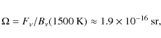
where
![\begin{figure}
\par\includegraphics[width=8.5cm,clip]{13840fg5.eps}
\end{figure}](/articles/aa/full_html/2010/09/aa13840-09/img34.png)
|
Figure 5:
K - L |
| Open with DEXTER | |
![\begin{figure}
\par\includegraphics[width=8.5cm,clip]{13840fg6.eps}
\end{figure}](/articles/aa/full_html/2010/09/aa13840-09/img35.png)
|
Figure 6:
K - 12.8 vs. K color-magnitude diagram of
T Tau Sa. The diamonds represent measurements in which the
Sa-Sb pair was spatially resolved in the K-band, crosses denote measurements in which we calculate the K-band magnitude of Sa from the total flux of T Tau S assuming Sb has K=8.6. The N-S pair was spatially resolved at 12.8 |
| Open with DEXTER | |
This velocity is much higher than the velocities one may expect in the
close environment of T Tau Sa. The Kepler speed at
0.24 AU, the absolute minimum distance from the star at which the
screen may be positioned in order to cover a region of 0.48 AU in
diameter, is ![]() 90 km s-1, assuming a mass of 2.2
90 km s-1, assuming a mass of 2.2 ![]() for Sa (Köhler 2008; Köhler et al. 2008). This velocity corresponds to a circular orbit, screens orbiting on eccentric orbits may reach velocities of up to
for Sa (Köhler 2008; Köhler et al. 2008). This velocity corresponds to a circular orbit, screens orbiting on eccentric orbits may reach velocities of up to ![]() 130 km s-1
at this distance. If the absorbing screen would be on an eccentric
orbit, though, it would itself become warmer and brighter at
12.8
130 km s-1
at this distance. If the absorbing screen would be on an eccentric
orbit, though, it would itself become warmer and brighter at
12.8 ![]() m
on closest approach, thus at least partially compensating for its own
dimming effect. Thus, extinction caused by a ``structure'' existing
within the disk, e.g. a warp or spiral arm, cannot be
responsible for the observed IR variability. Moreover,
the velocity dispersion within a molecular cloud is only
a few km s-1 (e.g. Larson 1981),
which excludes dust clouds in relatively close vicinity of the star,
but not directly related to it, as viable absorbing screens.
m
on closest approach, thus at least partially compensating for its own
dimming effect. Thus, extinction caused by a ``structure'' existing
within the disk, e.g. a warp or spiral arm, cannot be
responsible for the observed IR variability. Moreover,
the velocity dispersion within a molecular cloud is only
a few km s-1 (e.g. Larson 1981),
which excludes dust clouds in relatively close vicinity of the star,
but not directly related to it, as viable absorbing screens.
In the above analysis we have made several simplifications, which were all chosen to lower the required velocities for the observing screen, i.e. to favor the variable extinction scenario. The goal was to show that variable extinction can be ruled out, even with these unrealistically conservative assumptions:

- The required velocity of the obscuring screen that we derived
is the absolute minimum value that does not violate fundamental laws of
physics (Planck's or Kepler's law), under the assumption that the
observed IR continuum radiation is thermal dust emission. However, in
reality, the region of the disk that emits the bulk of the flux at
12.8 m
is likely much larger, leading to a correspondingly higher minimum
required velocity. For a typical disk model around an object with
approximately the stellar parameters of T Tau Sa, the
``size'' of the disk (here defined as the region within which 75%
of the flux at 12.8 m is emitted) is about 15 AU in radius (e.g. van Boekel et al. 2005).
In the special case of T Tau Sa, where the disk is likely
truncated on the outside at a radius of 3-5 AU due to tidal
interactions with T Tau Sb, the region we see at 12.8 m
probably encompasses the entire disk. Conservatively assuming an outer
radius of 3 AU for the disk, an absorbing screen would need to
travel at
 700 km s-1 in order to (un-) cover 26% of the emitting region within four days, whereas the Kepler velocity at this radius is only 26 km s-1.
-
- We assumed the absorbing screen to be 100% opaque at 12.8 m.
If the screen's transparency at this wavelength is considerable, a
larger area needs to be (un-) covered within the available time and the
required velocity becomes correspondingly higher.
Note that if we apply the same simple model to the fastest variations detected by Beck et al. (2004) at 2.2 ![]() m (
m (![]() 0.9 Jy in seven days)
0.9 Jy in seven days)![]() , we cannot exclude variable extinction: a 1500 K blackbody emitting the corresponding flux would have a diameter of
, we cannot exclude variable extinction: a 1500 K blackbody emitting the corresponding flux would have a diameter of ![]() 0.15 AU and the minimum speed needed for an opaque screen to (un-) cover this region within 7 days is only
0.15 AU and the minimum speed needed for an opaque screen to (un-) cover this region within 7 days is only ![]() 37 km s-1. This is substantially below the corresponding Kepler speed of
37 km s-1. This is substantially below the corresponding Kepler speed of ![]() 160 km s-1,
and thus variable extinction is a perfectly viable explanation for the
observed variations. Considering that the stellar photosphere may
contribute significantly to the total flux at 2.2
160 km s-1,
and thus variable extinction is a perfectly viable explanation for the
observed variations. Considering that the stellar photosphere may
contribute significantly to the total flux at 2.2 ![]() m, the case for variable extinction becomes even stronger. Only the long wavelength of our VISIR observations allows rejection of the variable extinction hypothesis.
m, the case for variable extinction becomes even stronger. Only the long wavelength of our VISIR observations allows rejection of the variable extinction hypothesis.
4.2 Can the observed long-term brightness fluctuations be caused by variable accretion?
In the previous section we showed that apparent brightness fluctuations due to variable extinction cannot be the cause of the observed short-term mid-IR photometric variations of T Tau Sa. Therefore the variability must be due to intrinsic changes in the luminosity of Sa. A high and strongly variable accretion rate would naturally lead to such luminosity changes in a young star like Sa, as already argued by Ghez et al. (1991). Thus, variable accretion is the prime candidate mechanism to explain the observed short-term variability. One may ask whether it can explain the observed long-term photometric variations, which are of much larger amplitude, as well. The variable accretion mechanism has previously been deemed unfit to explain the ``bluer when brighter'' color-magnitude behavior of the long-term brightness fluctuations (Beck et al. 2004). In this section we will show that constructing a disk model that qualitatively reproduces the observed color-magnitude behavior is in fact possible, with parameters that remain in a realistic range.
Our model of the Sa disk consists of two components: an ``active'' inner disk in which luminosity is generated by the release of gravitational energy from accreting material, and a ``passive'' outer disk that is irradiated by the central star and the inner disk, and reprocesses the absorbed optical/NIR photons into longer wavelength infrared radiation. The model parameters are briefly discussed here and are also listed in Table 5. They are chosen so that they represent Sa and its disk to the best of current knowledge. In particular the small outer radius of the disk and the near edge-on orientation are key features (e.g. Duchêne et al. 2005).
The active, inner part is modeled with an optically thick,
geometrically thin accretion disk with a radial temperature profile
following the Shakura & Sunyaev (1973)
model. In addition, a ``hot-spot'' covering 1% of the star,
representing the accretion shock of infalling material hitting the
stellar surface, is included by adding a blackbody of the corresponding
temperature and luminosity to the stellar spectrum. For the passive,
outer disk we used the 2D radiative transfer code RADMC (Dullemond & Dominik 2004) to calculate the temperature structure and emergent infrared SED. The passive disk part has an inner radius of
![]() = 0.5 AU, an outer radius of
= 0.5 AU, an outer radius of
![]() = 5 AU, a mass of
= 5 AU, a mass of
![]() = 10-3
= 10-3 ![]() (assuming a gas to dust ratio of 100) with a radial surface density profile of
(assuming a gas to dust ratio of 100) with a radial surface density profile of ![]()
![]() R-1, a flared geometry with a flaring index
R-1, a flared geometry with a flaring index![]() of
of ![]() = 2/7 and a scale height of H0 = 0.021 AU at the inner disk edge of the passive, re-processing disk (H/R = 0.042,
chosen to be the value corresponding to hydrostatic equilibrium in the
``high'' state). The outer radius is much smaller than that of typical
circumstellar disks because of tidal truncation by Sb, whose highly
eccentric orbit brings it to within
= 2/7 and a scale height of H0 = 0.021 AU at the inner disk edge of the passive, re-processing disk (H/R = 0.042,
chosen to be the value corresponding to hydrostatic equilibrium in the
``high'' state). The outer radius is much smaller than that of typical
circumstellar disks because of tidal truncation by Sb, whose highly
eccentric orbit brings it to within ![]() 12 AU from Sa at closest approach. This naturally explains the non-detection of the Sa disk at mm wavelengths by Hogerheijde et al. (1997) and Akeson et al. (1998), as argued before by Koresko (2000).
12 AU from Sa at closest approach. This naturally explains the non-detection of the Sa disk at mm wavelengths by Hogerheijde et al. (1997) and Akeson et al. (1998), as argued before by Koresko (2000).
By varying the accretion rate, we change the amount of energy that is
released in the center of the system, heating the circumstellar
material. The luminosity of the stellar photosphere dominates at low
accretion rates, providing a ``base level'' for the energy output. At
accretion rates above ![]() 7
7 ![]() 10-7
10-7 ![]() yr-1
accretion becomes the main energy source and the heating rate of the
circumstellar material scales roughly linearly with the accretion rate.
Variations in the central luminosity lead to essentially instantaneous
variations in the temperature of the circumstellar material and to
corresponding changes in the infrared emission because the dust grains
are small and attain their new equilibrium temperature practically
instantly if the radiation field changes, and the light travel time to
the outer disk edge is only about 30 min.
yr-1
accretion becomes the main energy source and the heating rate of the
circumstellar material scales roughly linearly with the accretion rate.
Variations in the central luminosity lead to essentially instantaneous
variations in the temperature of the circumstellar material and to
corresponding changes in the infrared emission because the dust grains
are small and attain their new equilibrium temperature practically
instantly if the radiation field changes, and the light travel time to
the outer disk edge is only about 30 min.
Table 5: Summary of the parameters of the radiative transfer model described in Sect. 4.2 and Figs. 5-7.
For the luminosity of the central star itself, we adopt a value of 10 ![]() .
This is lower by a factor of a few compared to the estimate by Duchêne et al. (2005), who base their value on a mass estimate of 2.5-3
.
This is lower by a factor of a few compared to the estimate by Duchêne et al. (2005), who base their value on a mass estimate of 2.5-3 ![]() for Sa. However, dynamical modeling of the Sa-Sb orbit including more recent data yields a mass estimate of
for Sa. However, dynamical modeling of the Sa-Sb orbit including more recent data yields a mass estimate of ![]() 2.2
2.2 ![]() for Sa (Köhler 2008; Köhler et al. 2008), which is essentially identical to the mass of T Tau N (2.1
for Sa (Köhler 2008; Köhler et al. 2008), which is essentially identical to the mass of T Tau N (2.1 ![]() ,
White & Ghez 2001). The bolometric luminosity of T Tau N is relatively well determined to be 7.3
+1.3-1.1
,
White & Ghez 2001). The bolometric luminosity of T Tau N is relatively well determined to be 7.3
+1.3-1.1 ![]() (White & Ghez 2001), and assuming the stars are co-eval therefore yields a luminosity of
(White & Ghez 2001), and assuming the stars are co-eval therefore yields a luminosity of ![]() 10
10 ![]() for
Sa. A lower stellar luminosity is favorable for a scenario in
which the IR variability is explained by variable accretion: the
required extra luminosity in ``high states'' is always relative to the
stellar photosphere and thus directly scales with the stellar
luminosity. The stellar parameters that we chose correspond to a
2 Myr-old star of 2.2
for
Sa. A lower stellar luminosity is favorable for a scenario in
which the IR variability is explained by variable accretion: the
required extra luminosity in ``high states'' is always relative to the
stellar photosphere and thus directly scales with the stellar
luminosity. The stellar parameters that we chose correspond to a
2 Myr-old star of 2.2 ![]() according to the pre-main sequence evolutionary tracks by Dotter et al. (2008).
according to the pre-main sequence evolutionary tracks by Dotter et al. (2008).
We performed model calculations for mass accretion rates of 10-8, 10-6, and 10-5 ![]() yr-1. For the lowest accretion rate, the accretion luminosity amounts to
yr-1. For the lowest accretion rate, the accretion luminosity amounts to ![]() 2%
of the stellar luminosity and the resulting fluxes are essentially
identical to those obtained with a zero accretion rate. We calculated
models for a range of nearly edge-on inclinations. Because our
objective is to demonstrate that a variable accretion model is in
principle capable of reproducing the observed color-magnitude behavior,
we searched for a model that gives a fair match to the observations but
did not comprehensively explore parameter space. A model with
parameters as listed earlier in this section and in Table 5, seen at an inclination of 74
2%
of the stellar luminosity and the resulting fluxes are essentially
identical to those obtained with a zero accretion rate. We calculated
models for a range of nearly edge-on inclinations. Because our
objective is to demonstrate that a variable accretion model is in
principle capable of reproducing the observed color-magnitude behavior,
we searched for a model that gives a fair match to the observations but
did not comprehensively explore parameter space. A model with
parameters as listed earlier in this section and in Table 5, seen at an inclination of 74![]() and with a foreground extinction of 15 mag agrees fairly well with
the observations (the extinction matches the value of the
foreground extinction observed toward Sb (Duchêne et al. 2005)).
This particular inclination yields the best fit for the set of model
parameters that we chose, but other choices of disk parameters will
result in slightly different best-fit inclinations. Thus, our model
does not accurately constrain the inclination of the Sa disk, but
we stress that a near edge-on inclination is required to obtain the
correct color-magnitude behavior of the variations, regardless of the
specific choice of disk parameters.
and with a foreground extinction of 15 mag agrees fairly well with
the observations (the extinction matches the value of the
foreground extinction observed toward Sb (Duchêne et al. 2005)).
This particular inclination yields the best fit for the set of model
parameters that we chose, but other choices of disk parameters will
result in slightly different best-fit inclinations. Thus, our model
does not accurately constrain the inclination of the Sa disk, but
we stress that a near edge-on inclination is required to obtain the
correct color-magnitude behavior of the variations, regardless of the
specific choice of disk parameters.
![\begin{figure}
\par\includegraphics[width=8.5cm,clip]{13840fg7-new.eps}
\end{figure}](/articles/aa/full_html/2010/09/aa13840-09/img51.png)
|
Figure 7: Observed infrared
photometry of Sa, with radiative transfer model SEDs over-plotted. The
photometry is the same as in Figs. 5 and 6. The model SED curves are for accretion rates of 10-5, 10-6, and 10-8 |
| Open with DEXTER | |
In Fig. 7 we show the model SEDs for accretion rates of 10-8, 10-6, and 10-5 ![]() yr-1,
as well as the observed infrared photometry. We also show the
model for the highest accretion rate as it would appear if the
foreground extinction is omitted (grey curve). In Figs. 5 and 6
we showed the observed color-magnitude behavior of the photometric
variations of Sa. The model magnitudes are over-plotted and labeled
with their respective accretion rates. The results of our modeling
efforts can be summarized as follows:
yr-1,
as well as the observed infrared photometry. We also show the
model for the highest accretion rate as it would appear if the
foreground extinction is omitted (grey curve). In Figs. 5 and 6
we showed the observed color-magnitude behavior of the photometric
variations of Sa. The model magnitudes are over-plotted and labeled
with their respective accretion rates. The results of our modeling
efforts can be summarized as follows:
-
- the near-infrared color and brightness variations are
qualitatively reproduced: we obtain a ``redder when fainter'' behavior
in a K - L
 vs. K color-magnitude plot (see Fig. 5). The slope of the relation in the model is somewhat shallower (i.e. closer to grey) than observed.
-
- the observed K-[12.8] vs. K color-magnitude behavior is qualitatively reproduced. The slope of the modeled relation fits the observations well. The considerable observed scatter can at least in part be attributed to the time lag between the near- and mid-infrared observations (see Fig. 6).
-
- the disk model always produces a 10 m silicate in emission, even at 90
 (edge-on) inclination. Additional foreground extinction is needed to explain the observed silicate absorption feature.
The variable accretion mechanism has been proposed previously,
based on the apparent grey behavior of the observed near- to
mid-infrared flux variations (Ghez et al. 1991; Duchêne et al. 2002). However, based on a much larger data set we show that the large, long-term flux variations at 2.2 and 12.8 ![]() m are accompanied by substantial color variations (Fig. 6),
which can be reproduced by our variable accretion model. However, these
data can also be explained with variable foreground extinction (see the
reddening vectors drawn in Figs. 5 and 6). The total amplitude of the foreground extinction required to cover the observed brightness range is
m are accompanied by substantial color variations (Fig. 6),
which can be reproduced by our variable accretion model. However, these
data can also be explained with variable foreground extinction (see the
reddening vectors drawn in Figs. 5 and 6). The total amplitude of the foreground extinction required to cover the observed brightness range is ![]()
![]()
![]() 40 mag.
40 mag.
4.2.1 Variable extinction causing variable disk-illumination?
In the previous paragraphs we showed that variable extinction in its simplest form, i.e. absorbing material passing in front of a source of approximately constant intrinsic luminosity, cannot cause the observed fast mid-IR brightness variations. However, the color-magnitude behavior of the large, multi-magnitude variations that have been observed during the last two decades, can be explained with variable extinction (see Sect. 4.2). The variable accretion model is in principle capable of explaining both the detected sub-magnitude fast variations, as well as the presumably slower multi-magnitude variations. Here we will consider a conceptually different realization of the variable extinction scheme, in which we attempt to explain both the short- and long-term variations with extinction alone.
To this purpose, we will introduce ``central extinction events'': variable absorption columns close to the central star that cause substantial changes in the illumination of the disk surface at larger radii with optical and near-infrared radiation. This could in principle lead to fast variations at mid-IR wavelengths because the material causing the variable disk illumination resides much closer to the central star than the material emitting the bulk of the mid-IR radiation, thereby circumventing the dynamical timescale problem encountered in the ``classical'' variable extinction scenario.
In order to explore this scheme in a more quantitative sense,
we constructed a passive disk model for Sa, in which we introduce
variable absorption columns by increasing the scale height at the inner
disk edge. The disk parameters![]() are the same as those of the model presented in Sect. 4.2, but as the central illuminating source we replaced the 10
are the same as those of the model presented in Sect. 4.2, but as the central illuminating source we replaced the 10 ![]() star plus variable accretion component with a star-only configuration with a constant luminosity of 40
star plus variable accretion component with a star-only configuration with a constant luminosity of 40 ![]() (Duchêne et al. 2005).
(Duchêne et al. 2005).
We considered both a scenario in which the scale height at the inner
disk edge is time variable, and one in which a fixed ``structure''
rotates at the inner disk edge with the Keplerian speed, casting a
shadow over the outer disk that rotates along with the same angular
velocity. For the former experiment, we artificially increased the
scale height of the disk between
![]() and 2
and 2
![]() ,
at all azimuthal angles. If we increase the scale height by 55%,
with respect to the disk parameters given in the previous paragraph,
the flux at 12.8
,
at all azimuthal angles. If we increase the scale height by 55%,
with respect to the disk parameters given in the previous paragraph,
the flux at 12.8 ![]() m decreases by 0.26 mag because the inner disk somewhat shadows the regions at larger radii. The
m decreases by 0.26 mag because the inner disk somewhat shadows the regions at larger radii. The ![]() 0.26 mag brightening at 12.8
0.26 mag brightening at 12.8 ![]() m
that we observed in February 2008 may conversely be explained by
the opposite change in inner rim structure: a reduction of the
pressure scale height from
m
that we observed in February 2008 may conversely be explained by
the opposite change in inner rim structure: a reduction of the
pressure scale height from ![]() 0.034 AU to
0.034 AU to ![]() 0.022 AU within
0.022 AU within ![]() 4 days. The height above the midplane where the disk becomes optically thin to the stellar irradiation
4 days. The height above the midplane where the disk becomes optically thin to the stellar irradiation![]() then decreases from
then decreases from ![]() 0.16 AU to
0.16 AU to ![]() 0.11 AU,
i.e. by more than twice the pressure scale height corresponding to
hydrostatic equilibrium. The orbital period at 0.5 AU from
a 2.2
0.11 AU,
i.e. by more than twice the pressure scale height corresponding to
hydrostatic equilibrium. The orbital period at 0.5 AU from
a 2.2 ![]() star is
star is ![]() 87 days,
and thus vertical movements on the order of one scale height require
roughly 20 days, which is much longer than our observational
constraint. Thus we conclude that changes in the inner disk structure
cannot cause the observed fast mid-IR brightness variations.
87 days,
and thus vertical movements on the order of one scale height require
roughly 20 days, which is much longer than our observational
constraint. Thus we conclude that changes in the inner disk structure
cannot cause the observed fast mid-IR brightness variations.
A somewhat different approach is to take a fixed enhancement of
the disk scale-height at the inner rim over only part of the azimuthal
range, causing a ``shadow'' to be cast over the disk behind it.
This shadow will move over the outer disk with an angular velocity
corresponding to the Kepler speed at the inner edge, and thus cause a
``cool region'' at larger radii that moves at locally vastly
super-keplerian velocities over the disk surface. For near edge-on
inclinations, where the mid-IR flux we see is dominated by the far side
of the disk, this can cause substantial dimming. We used the 3D version
of RADMC
(Dullemond et al., in prep.) to calculate light curves of a
system in which the scale height at the inner rim is increased with
respect to hydrostatic equilibrium over a limited azimuthal range![]() . With this we can achieve brightness variations of
. With this we can achieve brightness variations of ![]() 0.15 mag on timescales of
0.15 mag on timescales of ![]() 20 days.
Because the enhancement of the scale height is unrealistically large
and yet the brightness variations are substantially smaller and slower
than observed, we do not consider this scenario to be a viable
explanation for our observations.
20 days.
Because the enhancement of the scale height is unrealistically large
and yet the brightness variations are substantially smaller and slower
than observed, we do not consider this scenario to be a viable
explanation for our observations.
We conclude that variable accretion is the prime mechanism responsible for the observed short-term mid-IR variability, and exclude a significant role for variable extinction in this matter, as explained in Sect. 4.1.
The short-term near-IR photometric variations are naturally also
explained by variable accretion, though the existing data do not
strictly exclude variable extinction as their cause. Based on the
hitherto available data, both variable accretion and variable
extinction are viable mechanisms to explain the long-term
photometric variations and the associated color-magnitude behavior.
Data presented in past studies, in particular a time-variable optical
depth in the 3.05 ![]() m ice absorption feature (Beck et al. 2001), do suggest that at least part of the variability can be attributed to variable extinction.
m ice absorption feature (Beck et al. 2001), do suggest that at least part of the variability can be attributed to variable extinction.
4.2.2 The 10 m silicate feature in Sa
The fact that T Tau S shows a deep silicate absorption feature in the 10 ![]() m spectral region (Ghez et al. 1991), which was later shown to arise in Sa only (Ratzka et al. 2009; Skemer et al. 2008), has been regarded as evidence that the 10
m spectral region (Ghez et al. 1991), which was later shown to arise in Sa only (Ratzka et al. 2009; Skemer et al. 2008), has been regarded as evidence that the 10 ![]() m emission is dominated by a disk that is seen nearly edge-on from our vantage point (e.g. Duchêne et al. 2005).
Our radiative transfer model of the Sa disk, however, always shows a
silicate feature in emission, even for an edge-on inclination (see the
unreddened model curve in Fig. 7,
grey line). This is due to the ``artificial'' truncation of the Sa disk
by the tidal influence of Sb, with an outer radius of 5 AU in our
model. In ``normal'' T Tauri disks, which are much larger, cold
material in the outer disk regions obscures the warm inner disk when
viewed at near edge-on inclinations, causing a silicate feature in
absorption. In the special case of Sa, the entire disk is warm enough
to emit in the 10
m emission is dominated by a disk that is seen nearly edge-on from our vantage point (e.g. Duchêne et al. 2005).
Our radiative transfer model of the Sa disk, however, always shows a
silicate feature in emission, even for an edge-on inclination (see the
unreddened model curve in Fig. 7,
grey line). This is due to the ``artificial'' truncation of the Sa disk
by the tidal influence of Sb, with an outer radius of 5 AU in our
model. In ``normal'' T Tauri disks, which are much larger, cold
material in the outer disk regions obscures the warm inner disk when
viewed at near edge-on inclinations, causing a silicate feature in
absorption. In the special case of Sa, the entire disk is warm enough
to emit in the 10 ![]() m
spectral region. The radiation that we receive is dominated by the
optically thin upper disk layers, yielding a silicate feature in
emission, regardless of the viewing angle. Ratzka et al. (2009)
reach the same conclusion based on their radiative transfer model for
Sa using the MC3D code. Note that the shape and peak to continuum
ratio of the silicate band depend on the grain size used. The small,
sub-micron sized grains used in our model cause a relatively strong
emission band peaking just short-ward of 10
m
spectral region. The radiation that we receive is dominated by the
optically thin upper disk layers, yielding a silicate feature in
emission, regardless of the viewing angle. Ratzka et al. (2009)
reach the same conclusion based on their radiative transfer model for
Sa using the MC3D code. Note that the shape and peak to continuum
ratio of the silicate band depend on the grain size used. The small,
sub-micron sized grains used in our model cause a relatively strong
emission band peaking just short-ward of 10 ![]() m.
The use of larger grains results in a weaker, broader silicate feature,
and one can make the silicate band essentially disappear from the
spectrum by using very large (
m.
The use of larger grains results in a weaker, broader silicate feature,
and one can make the silicate band essentially disappear from the
spectrum by using very large (![]() 10
10 ![]() m)
grains. However, one never gets a silicate feature in absorption. Thus,
an additional, external absorption component needs to be invoked. This
is consistent with the fact that Sb, whose disk is thought to be seen
more or less face-on (e.g. Duchêne et al. 2005), suffers an extinction of
m)
grains. However, one never gets a silicate feature in absorption. Thus,
an additional, external absorption component needs to be invoked. This
is consistent with the fact that Sb, whose disk is thought to be seen
more or less face-on (e.g. Duchêne et al. 2005), suffers an extinction of ![]()
![]() 15 mag.
The shape of the observed silicate absorption feature implies that the
material causing the absorption consists predominantly of small (
15 mag.
The shape of the observed silicate absorption feature implies that the
material causing the absorption consists predominantly of small (![]() 1
1 ![]() m) grains.
m) grains.
4.3 A tentative scenario for T Tau Sa
The light curves shown in Fig. 4 can qualitatively be described as follows![]() .
From the beginning of the IR observations, in 1982, until 1989
T Tau S appears to have been in a ``low state''. Because
there are only three measurements in this period, it is by no means
certain that it has been faint during this whole period, but the
available measurements all show T Tau S to be of essentially
the same (low) brightness at 2.2
.
From the beginning of the IR observations, in 1982, until 1989
T Tau S appears to have been in a ``low state''. Because
there are only three measurements in this period, it is by no means
certain that it has been faint during this whole period, but the
available measurements all show T Tau S to be of essentially
the same (low) brightness at 2.2 ![]() m.
Sometime in 1989, the brightness of the southern component started to
increase strongly. Based on data from later epochs this increase, or at
least the vast majority of it, is attributed to Sa only. During the
period from
m.
Sometime in 1989, the brightness of the southern component started to
increase strongly. Based on data from later epochs this increase, or at
least the vast majority of it, is attributed to Sa only. During the
period from ![]() 1991 to
1991 to ![]() 1995 the temporal sampling was very poor, but the few available measurements suggest Sa to be relatively faint. From
1995 the temporal sampling was very poor, but the few available measurements suggest Sa to be relatively faint. From ![]() 1996 to late 2001 Sa has been in a ``high and variable'' state. This period has been very well sampled by Beck et al. (2004) and the K-band brightness varied between K
1996 to late 2001 Sa has been in a ``high and variable'' state. This period has been very well sampled by Beck et al. (2004) and the K-band brightness varied between K ![]() 7.5 mag and K
7.5 mag and K ![]() 6 mag. From late 2001 to late 2003 the brightness of Sa decreased to K
6 mag. From late 2001 to late 2003 the brightness of Sa decreased to K ![]() 10.5 mag.
The temporal coverage of the observations is poor and thus we cannot
assess how ``smooth'' this decrease was. Sometime between late 2004 and
late 2006 the brightness of Sa rose again to K
10.5 mag.
The temporal coverage of the observations is poor and thus we cannot
assess how ``smooth'' this decrease was. Sometime between late 2004 and
late 2006 the brightness of Sa rose again to K ![]() 9 mag, and is currently varying around this value.
9 mag, and is currently varying around this value.
In view of the variable accretion scenario, the dramatic brightening
events in the early and late 1990s and the interspersed episodes of
irregular flux variations, of which we may be seeing the last twitch at
the current time, could be interpreted as an ``outburst'' of accretion.
In this respect, it is particularly interesting to compare the timing
of the outburst with that of the periastron passage of the companion
Sb. In the current best-fit solution of the Sa-Sb orbit, the
closest approach occurred in June 1995, with an uncertainty of
somewhat more than a year (1![]() ), as we have indicated in Fig. 4
with a grey vertical band. Thus, we have a period of enhanced activity
around the time of closest approach of the companion, with the middle
of the active period timed somewhat after periastron passage, and the
strongest activity occurring in the second half of the active period.
We will now argue that this behavior provides a good qualitative match
to a scenario in which an accretion outburst in the center of the
Sa disk is induced by the gravitational influence of Sb, tidally
disturbing the Sa disk during periastron passage.
), as we have indicated in Fig. 4
with a grey vertical band. Thus, we have a period of enhanced activity
around the time of closest approach of the companion, with the middle
of the active period timed somewhat after periastron passage, and the
strongest activity occurring in the second half of the active period.
We will now argue that this behavior provides a good qualitative match
to a scenario in which an accretion outburst in the center of the
Sa disk is induced by the gravitational influence of Sb, tidally
disturbing the Sa disk during periastron passage.
When a young star and disk system has a low-mass companion, the
latter will tidally truncate the disk around the primary to ![]() 1/3 times the semi-major axis of the orbit (e.g. Artymowicz 1993).
If the companion is on an eccentric orbit, its gravitational
influence on the primary disk will be strongly time-dependent, being
relatively weak during most of the orbit but culminating near
periastron passage. Kley & Nelson (2008) modeled the close binary system
1/3 times the semi-major axis of the orbit (e.g. Artymowicz 1993).
If the companion is on an eccentric orbit, its gravitational
influence on the primary disk will be strongly time-dependent, being
relatively weak during most of the orbit but culminating near
periastron passage. Kley & Nelson (2008) modeled the close binary system ![]() Cephei
in its youth, which is thought to have been very similar to the Sa-Sb
system today. It has primary and secondary masses of
Cephei
in its youth, which is thought to have been very similar to the Sa-Sb
system today. It has primary and secondary masses of ![]() 1.59
1.59 ![]() and
and ![]() 0.38
0.38 ![]() ,
respectively, a semi-major axis of
,
respectively, a semi-major axis of ![]() 18 AU, and an eccentricity of
18 AU, and an eccentricity of ![]() 0.36 (Hatzes et al. 2003). In addition, the primary has a planetary companion with a mass of M sin i
0.36 (Hatzes et al. 2003). In addition, the primary has a planetary companion with a mass of M sin i ![]() 1.7
1.7
![]() (Hatzes et al. 2003), which is, however, not of central importance to the current discussion. Kley & Nelson (2008) performed hydro-dynamical simulations of the disk around the young
(Hatzes et al. 2003), which is, however, not of central importance to the current discussion. Kley & Nelson (2008) performed hydro-dynamical simulations of the disk around the young ![]() Cep
primary and considered the tidal effects of the low-mass secondary. The
simulations reveal a nearly undisturbed disk at most orbital phases,
when the companion is at relatively large distances. As the
companion approaches the primary, however, two strong spiral shock
waves are excited which propagate all the way to the inner disk
(see Fig. 8).
This takes some time, and therefore the gravitational disturbance of
the inner disk is not symmetrical in time with respect to the
periastron passage, but lags somewhat. The strongest disturbances at
the inner disk edge occur substantially after closest approach.
Cep
primary and considered the tidal effects of the low-mass secondary. The
simulations reveal a nearly undisturbed disk at most orbital phases,
when the companion is at relatively large distances. As the
companion approaches the primary, however, two strong spiral shock
waves are excited which propagate all the way to the inner disk
(see Fig. 8).
This takes some time, and therefore the gravitational disturbance of
the inner disk is not symmetrical in time with respect to the
periastron passage, but lags somewhat. The strongest disturbances at
the inner disk edge occur substantially after closest approach.
![\begin{figure}
\par\includegraphics[width=8.5cm,clip]{13840fg8.eps}
\end{figure}](/articles/aa/full_html/2010/09/aa13840-09/img57.png)
|
Figure 8: Two-dimensional temperature distribution of the Sa disk 10.8 yrs after the periastron passage of Sb, for a hydrodynamic simulation using the physical parameters of the T Tau S system. X and Y are spatial coordinates, and the disk is viewed face-on in this representation. To better bring out the entire range of temperatures we show T[K]1/4, the colors cover the temperature range of 10 to 2000 K. For a color version of this figure see the electronic version of this journal. |
| Open with DEXTER | |
We speculate that such shock waves induce enhanced accretion in the
innermost disk region of Sa when Sb is near periastron.
For example, the mechanical energy dissipated in the shocks may
cause a normally essentially neutral disk medium to be sufficiently
ionized for MRI to become effective, naturally leading to strongly
enhanced accretion. We have re-run the Kley & Nelson model
including viscous heating and radiative cooling for the parameters of
the Sa-Sb system, and find the same behavior as seen in the ![]() Cep calculations
Cep calculations![]() .
The simulations provide a good qualitative match to the observations: a
period of enhanced accretion activity near every periastron passage,
whose peak has a substantial time lag with respect to the closest
approach of the secondary. Quantitatively, the model shows much
more modest variations in the accretion rate than inferred by the
observations, and the time between periastron passage and maximum
accretion activity is longer in the simulations by a factor of
.
The simulations provide a good qualitative match to the observations: a
period of enhanced accretion activity near every periastron passage,
whose peak has a substantial time lag with respect to the closest
approach of the secondary. Quantitatively, the model shows much
more modest variations in the accretion rate than inferred by the
observations, and the time between periastron passage and maximum
accretion activity is longer in the simulations by a factor of ![]() 3.
The Kley & Nelson model focuses on the dynamical evolution and mass
loss of the disk at its outer edge, but does not attempt to treat the
accretion physics at the inner disk edge in detail. A model with a
more detailed treatment of the disk viscosity and accretion physics in
the innermost disk regions is needed, which allows the spiral shock
waves to propagate inward more quickly and can account for the required
high accretion rates. This is beyond the scope of the current work, and
whether our qualitative model can be refined to provide a quantitative
match to the observations once all the relevant physics are included
remains to be confirmed.
3.
The Kley & Nelson model focuses on the dynamical evolution and mass
loss of the disk at its outer edge, but does not attempt to treat the
accretion physics at the inner disk edge in detail. A model with a
more detailed treatment of the disk viscosity and accretion physics in
the innermost disk regions is needed, which allows the spiral shock
waves to propagate inward more quickly and can account for the required
high accretion rates. This is beyond the scope of the current work, and
whether our qualitative model can be refined to provide a quantitative
match to the observations once all the relevant physics are included
remains to be confirmed.
Here we pose the companion-induced accretion outburst as an
idea to explain the observed behavior of T Tau S during the
past decades, and provide a clear prediction that can be easily
verified observationally: if this scenario is correct, Sa should return
to its ``low state'' some time in the near future, and stay there until
the next periastron passage of Sb. Exactly how long it will take for Sa
to return to ``quiescence'' in detail depends on the actual accretion
physics and inner disk parameters, neither of which we know. Thus,
while it is technically trivial to test the proposed scenario with
currently available observing facilities, it may in practice take a
substantial number of years to convincingly falsify our scheme.
Supportive evidence could be built up over the years if Sa is observed
to remain faint, the final prove may come only many years from now if
the next outburst coincides with the next periastron passage. The
current astrometric data still allow a wide range of orbital periods,
from ![]() 25 to
25 to ![]() 100 years,
but as new observations accumulate over the coming years, we should be
able to fairly accurately predict the onset of the next outburst long
before it would occur.
100 years,
but as new observations accumulate over the coming years, we should be
able to fairly accurately predict the onset of the next outburst long
before it would occur.
4.4 Issues
Here we briefly discuss some issues that are relevant to the current discussion.
4.4.1 The mass and lifetime of the Sa disk
The amount of material that we can reasonable assume to be present in the Sa disk is at most a few times 10-3 ![]() .
If the average accretion rate during an outburst is 5
.
If the average accretion rate during an outburst is 5 ![]() 10-6
10-6 ![]() yr-1 and an outburst lasts for 10 years, we can have only on the order of 102
these events before the disk is all gone, unless the Sa disk can
be supplied with fresh material. If the orbital period of Sa-Sb is
50 yrs, this means the current situation can exist for only
yr-1 and an outburst lasts for 10 years, we can have only on the order of 102
these events before the disk is all gone, unless the Sa disk can
be supplied with fresh material. If the orbital period of Sa-Sb is
50 yrs, this means the current situation can exist for only ![]() 5000 yrs.
Possibly the Sa-Sb pair became a close binary only within the last
several thousand years due to gravitational interaction with a third
object. It may also be possible that the Sa disk is still supplied
with fresh material coming in at high latitudes with respect to the
orbital plane as the Sa-Sb pair moves through ambient cloud
material. Because the disks of Sa and Sb appear strongly misaligned (Ratzka et al. 2009; Duchêne et al. 2005), the Sa disk and the Sa-Sb orbit are misaligned, and cloud material is present close to the Sa-Sb system (Sect. 3.2.3, Herbst et al. 2007; Gustafsson et al. 2008; Beck et al. 2008), the notion that cloud material is still being freshly supplied to the Sa disk is realistic.
5000 yrs.
Possibly the Sa-Sb pair became a close binary only within the last
several thousand years due to gravitational interaction with a third
object. It may also be possible that the Sa disk is still supplied
with fresh material coming in at high latitudes with respect to the
orbital plane as the Sa-Sb pair moves through ambient cloud
material. Because the disks of Sa and Sb appear strongly misaligned (Ratzka et al. 2009; Duchêne et al. 2005), the Sa disk and the Sa-Sb orbit are misaligned, and cloud material is present close to the Sa-Sb system (Sect. 3.2.3, Herbst et al. 2007; Gustafsson et al. 2008; Beck et al. 2008), the notion that cloud material is still being freshly supplied to the Sa disk is realistic.
4.4.2 A note on the Sb disk
Like the primary star Sa, the low-mass companion Sb also shows a
substantial infrared excess, indicating that some circumstellar
material is still present, presumably also in a small circumstellar
disk. As our calculations show, Sb will strongly disturb the Sa
disk during periastron passage. Conversely, the gravitational pull of
Sa will affect the disk around Sb even more strongly, and accretion
onto Sb should also be enhanced during periastron passage. Therefore
one may wonder why the observed brightness variations are much smaller
in Sb (maximum amplitude ![]() 0.4 mag RMS = 0.2 mag) than in Sa (amplitude
0.4 mag RMS = 0.2 mag) than in Sa (amplitude ![]() 3 mag).
3 mag).
Duchêne et al. (2002,2005) measured the Br ![]() line flux of Sb to be 7.2
line flux of Sb to be 7.2 ![]() 10-17 Wm-2 on 2000 November 19, and 9.4
10-17 Wm-2 on 2000 November 19, and 9.4 ![]() 10-17 Wm-2 on 2003 December 12, with corresponding K-band continuum magnitudes of 8.77 and 8.50, respectively. the spectral type of Sb corresponds to
10-17 Wm-2 on 2003 December 12, with corresponding K-band continuum magnitudes of 8.77 and 8.50, respectively. the spectral type of Sb corresponds to
![]()
![]() 3800 K (Duchêne et al. 2005), and assuming an age of 2 Myr this yields a mass of approximately 0.6
3800 K (Duchêne et al. 2005), and assuming an age of 2 Myr this yields a mass of approximately 0.6 ![]() and a luminosity of
and a luminosity of ![]() 0.45
0.45 ![]() by comparison to the pre-main sequence evolutionary tracks of Dotter et al. (2008), which seem reasonable. The corresponding stellar radius of Sb is R* = 1.55
by comparison to the pre-main sequence evolutionary tracks of Dotter et al. (2008), which seem reasonable. The corresponding stellar radius of Sb is R* = 1.55 ![]() .
Assuming a foreground extinction of
.
Assuming a foreground extinction of
![]() = 15 mag, a standard extinction law (
= 15 mag, a standard extinction law (
![]() = 0.112
= 0.112
![]() ), the relation between Br
), the relation between Br ![]() luminosity and accretion luminosity given in Eq. (3) of Calvet et al. (2004), and using the approximate relation
luminosity and accretion luminosity given in Eq. (3) of Calvet et al. (2004), and using the approximate relation
![]() = GM*
= GM*
![]() /R*, one derives mass accretion rates of 3.5
/R*, one derives mass accretion rates of 3.5 ![]() 10-8
10-8 ![]() yr-1 and 4.4
yr-1 and 4.4 ![]() 10-8
10-8 ![]() yr-1
for the respective epochs. The corresponding accretion luminosities are
approximately equal to the stellar luminosity. Therefore, variable
accretion is a viable mechanism for the observed modest near-infrared
variations in Sb as well. How variations in the accretion luminosity
translate to variations in the near-infrared continuum excess emission
is somewhat dependent on the disk structure: the extra luminosity is
released in the UV which cannot be observed due to the high extinction,
and we only see the reprocessed radiation from the hot inner disk
regions.
yr-1
for the respective epochs. The corresponding accretion luminosities are
approximately equal to the stellar luminosity. Therefore, variable
accretion is a viable mechanism for the observed modest near-infrared
variations in Sb as well. How variations in the accretion luminosity
translate to variations in the near-infrared continuum excess emission
is somewhat dependent on the disk structure: the extra luminosity is
released in the UV which cannot be observed due to the high extinction,
and we only see the reprocessed radiation from the hot inner disk
regions.
We note, however, that the existing data also perfectly agree with a
time variable extinction towards Sb. Between the aforementioned epochs of Br ![]() spectroscopy by Duchêne et al. the extinction would have decreased by
spectroscopy by Duchêne et al. the extinction would have decreased by ![]()
![]()
![]() 2.4 mag, assuming a standard extinction law.
2.4 mag, assuming a standard extinction law.
4.4.3 Mid-infrared brightness during the peak of the outburst
We are not aware of mid-IR measurements performed between roughly
1998 January and 2001 November, but we argue Sa must have been
very bright during that period, peaking at ![]() 40 Jy at 12.8
40 Jy at 12.8 ![]() m.
Should any mid-IR observations have been performed during this period,
they are highly relevant to the current discussion. The variable
extinction scenario predicts a lower peak-brightness in mid-IR than the
variable accretion scenario. However, only if mid-IR observations have
been performed (near-) simultaneously with the existing K-band
data they may provide supportive evidenced for either scenario. In case
of a substantial time lag the potential short-term variations will
inhibit drawing firm conclusions.
m.
Should any mid-IR observations have been performed during this period,
they are highly relevant to the current discussion. The variable
extinction scenario predicts a lower peak-brightness in mid-IR than the
variable accretion scenario. However, only if mid-IR observations have
been performed (near-) simultaneously with the existing K-band
data they may provide supportive evidenced for either scenario. In case
of a substantial time lag the potential short-term variations will
inhibit drawing firm conclusions.
5 Summary
The southern infrared companion of T Tau is a close binary
system of which the more massive member, T Tau Sa, shows
strong long-term photometric variability, with an amplitude of ![]() 3 mag at 2.2
3 mag at 2.2 ![]() m and
m and ![]() 2 mag in the 10
2 mag in the 10 ![]() m region on timescales of years. Short-term variability of
m region on timescales of years. Short-term variability of ![]() 1 mag within one week has been detected at 2.2
1 mag within one week has been detected at 2.2 ![]() m.
The physical mechanism driving the observed flux variations has been
under debate, the originally proposed intrinsic luminosity variations
due to a variable accretion rate have later been challenged in favor of
apparent brightness fluctuations due to variable foreground extinction.
m.
The physical mechanism driving the observed flux variations has been
under debate, the originally proposed intrinsic luminosity variations
due to a variable accretion rate have later been challenged in favor of
apparent brightness fluctuations due to variable foreground extinction.
We revisited the nature of the photometric variability of
T Tau Sa using new observations in the mid-infrared. In
February 2008 we detected a very fast increase of the mid-IR
brightness of T Tau S which can be attributed to Sa: +26 ![]() 2% at 12.8
2% at 12.8 ![]() m in 3.94 days. Using simple geometric arguments and basic physic laws we can exclude that this short-term
variability is due to time-variable extinction. We show that the fast
brightness fluctuations must instead reflect changes in intrinsic
luminosity, and attribute these to variable accretion. The key aspect
of our argument is the short timescale of the variations in combination
with the long observing wavelength.
m in 3.94 days. Using simple geometric arguments and basic physic laws we can exclude that this short-term
variability is due to time-variable extinction. We show that the fast
brightness fluctuations must instead reflect changes in intrinsic
luminosity, and attribute these to variable accretion. The key aspect
of our argument is the short timescale of the variations in combination
with the long observing wavelength.
We show that variable accretion can plausibly explain also the much larger long-term variability and its associated near-infrared ``bluer when brighter'' color-magnitude behavior, by creating a 2D radiative transfer disk model of the Sa disk that qualitatively reproduces the observed properties. However, the hitherto observed long-term variability can also be explained within the variable foreground-extinction scenario. A combination of both mechanisms, variable accretion and variable foreground extinction, may be required to explain the collective photometric variability of T Tau Sa.
In view of the tentative scenario that both the short- and
long-term variability of Sa are caused by variable accretion, we
reviewed the infrared light curve in relation to the parameters of the
Sa-Sb orbit. We propose that the dramatic brightening events in the
early and late 1990s and the interspersed episodes of irregular flux
variations were an accretion outburst, induced by gravitational
perturbation of the Sa disk during the periastron passage of Sb, with
closest approach in ![]() 1995. The induced maximum accretion rate is on the order of 10-5
1995. The induced maximum accretion rate is on the order of 10-5 ![]() yr-1.
While we do not model the physics of this outburst in detail, we make a
clear observational prediction: if this scheme is correct, Sa should
return to ``quiescence'' some time in the near future, and remain in a
low state until the next periastron passage of Sb.
yr-1.
While we do not model the physics of this outburst in detail, we make a
clear observational prediction: if this scheme is correct, Sa should
return to ``quiescence'' some time in the near future, and remain in a
low state until the next periastron passage of Sb.
We thank the ESO staff for executing the VISIR observations in service mode. R.v.B. thanks Kees Dullemond for many insightful discusisons. An anonymous referee is gratefully acknowledged for a detailed and constructively critical report, from which the manuscript greatly benefited.
References
- Akeson, R. L., Koerner, D. W., & Jensen, E. L. N. 1998, ApJ, 505, 358 [NASA ADS] [CrossRef] [Google Scholar]
- Ambartsumian, V. A. 1947, Stellar Evolution and Astrophysics (Erevan: Acad. Sci. Armenian S. S. R.) [Google Scholar]
- Ambartsumian, V. A. 1949, AZh, 26, 3 [Google Scholar]
- Artymowicz, P. 1993, ApJ, 419, 166 [NASA ADS] [CrossRef] [Google Scholar]
- Beck, T. L., & Simon, M. 2001, AJ, 122, 413 [NASA ADS] [CrossRef] [Google Scholar]
- Beck, T. L., Prato, L., & Simon, M. 2001, ApJ, 551, 1031 [NASA ADS] [CrossRef] [Google Scholar]
- Beck, T. L., Schaefer, G. H., Simon, M., et al. 2004, ApJ, 614, 235 [NASA ADS] [CrossRef] [Google Scholar]
- Beck, T. L., McGregor, P. J., Takami, M., & Pyo, T.-S. 2008, ApJ, 676, 472 [NASA ADS] [CrossRef] [Google Scholar]
- Beckwith, S., Skrutskie, M. F., Zuckerman, B., & Dyck, H. M. 1984, ApJ, 287, 793 [NASA ADS] [CrossRef] [Google Scholar]
- Brandner, W., Rousset, G., Lenzen, R., et al. 2002, The Messenger, 107, 1 [Google Scholar]
- Calvet, N., Hartmann, L., & Strom, S. E. 1997, ApJ, 481, 912 [NASA ADS] [CrossRef] [Google Scholar]
- Calvet, N., Muzerolle, J., Briceño, C., et al. 2004, AJ, 128, 1294 [NASA ADS] [CrossRef] [Google Scholar]
- Cohen, M., Walker, R. G., Carter, B., et al. 1999, AJ, 117, 1864 [NASA ADS] [CrossRef] [Google Scholar]
- Diolaiti, E., Bendinelli, O., Bonaccini, D., et al. 2000, A&AS, 147, 335 [NASA ADS] [CrossRef] [EDP Sciences] [Google Scholar]
- Dotter, A., Chaboyer, B., Jevremovic, D., et al. 2008, ApJS, 178, 89 [NASA ADS] [CrossRef] [Google Scholar]
- Duchêne, G., Ghez, A. M., & McCabe, C. 2002, ApJ, 568, 771 [NASA ADS] [CrossRef] [Google Scholar]
- Duchêne, G., Ghez, A. M., McCabe, C., & Ceccarelli, C. 2005, ApJ, 628, 832 [NASA ADS] [CrossRef] [Google Scholar]
- Duchêne, G., Beust, H., Adjali, F., Konopacky, Q. M., & Ghez, A. M. 2006, A&A, 457, L9 [NASA ADS] [CrossRef] [EDP Sciences] [Google Scholar]
- Dullemond, C. P., & Dominik, C. 2004, A&A, 417, 159 [NASA ADS] [CrossRef] [EDP Sciences] [Google Scholar]
- Dyck, H. M., Simon, T., & Zuckerman, B. 1982, ApJ, 255, L103 [NASA ADS] [CrossRef] [Google Scholar]
- Furlan, E., Forrest, W. J., Watson, D. M., et al. 2003, ApJ, 596, L87 [NASA ADS] [CrossRef] [Google Scholar]
- Ghez, A. M., Neugebauer, G., Gorham, P. W., et al. 1991, AJ, 102, 2066 [NASA ADS] [CrossRef] [Google Scholar]
- Gustafsson, M., Labadie, L., Herbst, T. M., & Kasper, M. 2008, A&A, 488, 235 [NASA ADS] [CrossRef] [EDP Sciences] [Google Scholar]
- Hatzes, A. P., Cochran, W. D., Endl, M., et al. 2003, ApJ, 599, 1383 [NASA ADS] [CrossRef] [Google Scholar]
- Herbst, W., Herbst, D. K., Grossman, E. J., & Weinstein, D. 1994, AJ, 108, 1906 [NASA ADS] [CrossRef] [Google Scholar]
- Herbst, T. M., Robberto, M., & Beckwith, S. V. W. 1997, AJ, 114, 744 [NASA ADS] [CrossRef] [Google Scholar]
- Herbst, T. M., Hartung, M., Kasper, M. E., Leinert, C., & Ratzka, T. 2007, AJ, 134, 359 [NASA ADS] [CrossRef] [Google Scholar]
- Hogerheijde, M. R., van Langevelde, H. J., Mundy, L. G., Blake, G. A., & van Dishoeck, E. F. 1997, ApJ, 490, L99 [NASA ADS] [CrossRef] [Google Scholar]
- Joy, A. H. 1945, ApJ, 102, 168 [NASA ADS] [CrossRef] [Google Scholar]
- Kasper, M. E., Feldt, M., Herbst, T. M., et al. 2002, ApJ, 568, 267 [NASA ADS] [CrossRef] [Google Scholar]
- Kley, W., & Nelson, R. P. 2008, A&A, 486, 617 [NASA ADS] [CrossRef] [EDP Sciences] [Google Scholar]
- Kobayashi, N., Nagata, T., Hodapp, K.-W., & Hora, J. L. 1994, PASJ, 46, L183 [NASA ADS] [Google Scholar]
- Köhler, R. 2008, J. Phys. Conf. Ser., 131, 012028 [Google Scholar]
- Köhler, R., Ratzka, T., Herbst, T. M., & Kasper, M. 2008, A&A, 482, 929 [NASA ADS] [CrossRef] [EDP Sciences] [Google Scholar]
- Koresko, C. D. 2000, ApJ, 531, L147 [NASA ADS] [CrossRef] [PubMed] [Google Scholar]
- Kuhi, L. V. 1974, A&AS, 15, 47 [NASA ADS] [Google Scholar]
- Lagage, P. O., Pel, J. W., Authier, M., et al. 2004, The Messenger, 117, 12 [NASA ADS] [Google Scholar]
- Larson, R. B. 1981, MNRAS, 194, 809 [NASA ADS] [CrossRef] [Google Scholar]
- Loinard, L., Torres, R. M., Mioduszewski, A. J., et al. 2007, ApJ, 671, 546 [NASA ADS] [CrossRef] [Google Scholar]
- Lord, S. D. 1992, NASA Technical Memorandum, 103957 [Google Scholar]
- Lozinskii, A. M. 1949, Perem. Zvezdy, 7, 76 [Google Scholar]
- Maihara, T., & Kataza, H. 1991, A&A, 249, 392 [NASA ADS] [Google Scholar]
- Mel'nikov, S. Y., & Grankin, K. N. 2005, Astron. Lett., 31, 427 [NASA ADS] [CrossRef] [Google Scholar]
- Przygodda, F., van Boekel, R., Àbrahàm, P., et al. 2003, A&A, 412, L43 [NASA ADS] [CrossRef] [EDP Sciences] [Google Scholar]
- Ratzka, T., Schegerer, A. A., Leinert, C., et al. 2009, A&A, 502, 623 [NASA ADS] [CrossRef] [EDP Sciences] [Google Scholar]
- Reimann, H., Weinert, U., & Wagner, S. 1998, in Infrared Astronomical Instrumentation, ed. A. M. Fowler, Proc. SPIE, 3354, 865 [Google Scholar]
- Rieke, G. H., & Lebofsky, M. J. 1985, ApJ, 288, 618 [NASA ADS] [CrossRef] [Google Scholar]
- Roddier, F., Roddier, C., Brandner, W., et al. 2000, in IAU Symp., 200, 60P [Google Scholar]
- Shakura, N. I., & Sunyaev, R. A. 1973, A&A, 24, 337 [NASA ADS] [Google Scholar]
- Simon, M., Longmore, A. J., Shure, M. A., & Smillie, A. 1996, ApJ, 456, L41 [Google Scholar]
- Skemer, A. J., Close, L. M., Hinz, P. M., et al. 2008, ApJ, 676, 1082 [NASA ADS] [CrossRef] [Google Scholar]
- Stapelfeldt, K. R., Burrows, C. J., Krist, J. E., et al. 1998, ApJ, 508, 736 [NASA ADS] [CrossRef] [Google Scholar]
- Tessier, E., Bouvier, J., & Lacombe, F. 1994, A&A, 283, 827 [NASA ADS] [Google Scholar]
- van Boekel, R., Dullemond, C. P., & Dominik, C. 2005, A&A, 441, 563 [Google Scholar]
- van Boekel, R., Güdel, M., Henning, T., Lahuis, F., & Pantin, E. 2009, A&A, 497, 137 [NASA ADS] [CrossRef] [EDP Sciences] [Google Scholar]
- van den Ancker, M. E., Wesselius, P. R., Tielens, A. G. G. M., van Dishoeck, E. F., & Spinoglio, L. 1999, A&A, 348, 877 [NASA ADS] [Google Scholar]
- White, R. J., & Ghez, A. M. 2001, ApJ, 556, 265 [Google Scholar]
Footnotes
- ... T Tauri S
- Based on observations obtained at ESO's La Silla/Paranal observatory under programmes 280.C-5035, 068.D-0537, 070.C-0544, 070.C-0162, 072.C-0593, 074.C-0699, 074.C-0396, 078.C-0386, 380.C-0179, 382.C-0324, and 084.C-0783, as well as observations obtained at UKIRT.
- ... cube
- The T Tau system is very bright, allowing the beam shape
in each individual frame to be assessed. Both T Tau N and
T Tau S were detected at >100
 in every frame.
- ... circle
- The argument is qualitatively independent of the exact shape of the emitting region and we adopt the simplest possible geometry.
- ... days)
- The brightness of T Tau S increases from K = 7.4 mag on 1997 December 6 to K = 6.5 mag seven days later (Beck et al. 2004). Assuming Sb was constant at K = 8.6 mag, this implies that Sa went from K = 7.84 mag to K = 6.67 mag, i.e. it brightened by 1.2 mag, or 0.9 Jy.
- ... index
- The flaring index
 is defined so that the ratio of the disk scale height H and the distance to the central star R scales like H/R
 .
.
- ... parameters
-
 = 0.5 AU,
 = 5 AU,
 = 10-3
  ,
,
 R-1, = 2/7, H0 = 0.021 AU at 0.5 AU.
- ... irradiation
- Here this is taken to be the height where the optical depth in the radial direction at
 = 0.55 m falls below unity.
- ... range
- Over
 radians in azimuth the scale height is increased with a sinusoidal
shape, so that at the central azimuthal angle the scale height is
twice the hydrostatic value, and at angles of
radians in azimuth the scale height is increased with a sinusoidal
shape, so that at the central azimuthal angle the scale height is
twice the hydrostatic value, and at angles of  /2 and
  /2 with respect to the maximum it reaches the hydrostatic value.
- ... follows
- We will describe the K-band light curve because it has the best temporal sampling. The L
and 12.8 m light curves follow the K-band (see also Figs. 5 and 6).
- ... calculations
- Note that the model discussed here and shown in Fig. 8 is a hydrodynamical calculation and is independent of the radiative transfer model discussed in Sect. 4.2.
All Tables
Table 1: Summary of the VLT/VISIR observations.
Table 2:
UKIRT/MAX photometry of the T Tau system at 12.4 ![]() m.
m.
Table 3:
Summary of the VLT/NACO photometry in the ![]() band obtained between 2001 December and 2009 October.
band obtained between 2001 December and 2009 October.
Table 4: References for infrared photometry used in Figs. 4-6.
Table 5: Summary of the parameters of the radiative transfer model described in Sect. 4.2 and Figs. 5-7.
All Figures
| |
Figure 1:
Two-epoch VISIR imaging of the T Tau system in a narrow band filter centered on 12.81 |
| Open with DEXTER | |
| In the text | |
|
|
Figure 2:
PSF photometry (squares) and PSF spectroscopy performed with TIMMI2 in
2002. The northern and southern components are spatially marginally
resolved ( |
| Open with DEXTER | |
| In the text | |
|
|
Figure 3: Spatially extended K-band emission around Sa. Shown is a contour plot of the NACO images after subtraction of the best-fit point sources for T Tau N, Sa, and Sb (see Sects. 2.2.3 and 3.2.3 for details). All epochs were aligned and centered on Sa. + signs mark the positions of Sa and Sb. The inset shows the PSF with the 13.26 mas pixels of the s13 camera on the same scale as the main plot. The dashed contours show the best-fit point source of Sa, drawn at 25% and 75% of the Sa peak flux. |
| Open with DEXTER | |
| In the text | |
|
|
Figure 4:
Updated light curves of various components of the
T Tau system at various infrared wavelengths. References for
all measurements shown are given in Table 4. At the top (roughly between 0 and 3 mag) are N-band
measurements. Two epochs in which the observations were space based and
did not spatially resolve the N-S pair are indicated with
``1'' sub-scripts. The two epochs of TIMMI 2 observations
that only very marginally resolve the N-S pair are marked with
``2'' sub-scripts. In red we plot the total system brightness
(N+S), in black we plot the magnitude of the T Tau S (sum of
Sa and Sb). In the middle of the graph (roughly between 3 and 6 mag) we show L |
| Open with DEXTER | |
| In the text | |
|
|
Figure 5:
K - L |
| Open with DEXTER | |
| In the text | |
|
|
Figure 6:
K - 12.8 vs. K color-magnitude diagram of
T Tau Sa. The diamonds represent measurements in which the
Sa-Sb pair was spatially resolved in the K-band, crosses denote measurements in which we calculate the K-band magnitude of Sa from the total flux of T Tau S assuming Sb has K=8.6. The N-S pair was spatially resolved at 12.8 |
| Open with DEXTER | |
| In the text | |
|
|
Figure 7: Observed infrared
photometry of Sa, with radiative transfer model SEDs over-plotted. The
photometry is the same as in Figs. 5 and 6. The model SED curves are for accretion rates of 10-5, 10-6, and 10-8 |
| Open with DEXTER | |
| In the text | |
|
|
Figure 8: Two-dimensional temperature distribution of the Sa disk 10.8 yrs after the periastron passage of Sb, for a hydrodynamic simulation using the physical parameters of the T Tau S system. X and Y are spatial coordinates, and the disk is viewed face-on in this representation. To better bring out the entire range of temperatures we show T[K]1/4, the colors cover the temperature range of 10 to 2000 K. For a color version of this figure see the electronic version of this journal. |
| Open with DEXTER | |
| In the text | |
Copyright ESO 2010
Current usage metrics show cumulative count of Article Views (full-text article views including HTML views, PDF and ePub downloads, according to the available data) and Abstracts Views on Vision4Press platform.
Data correspond to usage on the plateform after 2015. The current usage metrics is available 48-96 hours after online publication and is updated daily on week days.
Initial download of the metrics may take a while.