| Issue |
A&A
Volume 517, July 2010
|
|
|---|---|---|
| Article Number | A19 | |
| Number of page(s) | 15 | |
| Section | Interstellar and circumstellar matter | |
| DOI | https://doi.org/10.1051/0004-6361/200913828 | |
| Published online | 27 July 2010 | |
The origin, excitation, and evolution of subarcsecond
outflows near T Tauri![[*]](/icons/foot_motif.png)
M. Gustafsson1 - L. E. Kristensen2 - M. Kasper3 - T. M. Herbst1,4
1 - Max Planck Institute for Astronomy, Königstuhl 17, 69117 Heidelberg, Germany
2 - Leiden Observatory, Leiden University, PO Box 9513, 2300 RA Leiden, The Netherlands
3 - European Southern Observatory, Karl-Schwarzschild-Str. 2, 85748 Garching, Germany
4 - Herzberg Institute of Astrophysics, National Research Council of Canada, Victoria, BC V9E 2E7, Canada
Received 8 December 2009 / Accepted 7 April 2010
Abstract
Aims. We study the complex H2 outflows in the
inner 300 AU of the young triple star system T Tauri, with
the goal of understanding the origin, excitation and evolution of the
circumstellar matter.
Methods. Using high spatial resolution, integral-field spectroscopy in the J and K photometric bands from SINFONI/VLT, we trace the spatial distribution of 12 H2
ro-vibrational emission lines, as well as one forbidden Fe II line. The
ratio of line strengths provides a two-dimensional view of both the
variable extinction and excitation temperature in this region, while
the line-center velocities, coupled with previously published imagery,
allow an assessment of the 3D space velocities and evolution of the
outflows.
Results. Several spatially distinct flows - some with a bow shock structure - appear within 1
![]() 5
of the stars. Data taken two years apart clearly show the evolution of
these flows. Some structures move and evolve, while others are
stationary in the plane of the sky. The two-dimensional extinction map
shows that the extinction between T Tau N and T Tau S is
very high. In addition to being clumpy the extincting material forms
part of a filament that extends to the east of the stars. In areas with
strong line emission, the v=1-0 S(1)/v=2-1 S(1) line ratio ranges from 8 to 20, indicating that all of the observed H2 is shock excited. The outflows in the immediate vicinity of T Tau S span
5
of the stars. Data taken two years apart clearly show the evolution of
these flows. Some structures move and evolve, while others are
stationary in the plane of the sky. The two-dimensional extinction map
shows that the extinction between T Tau N and T Tau S is
very high. In addition to being clumpy the extincting material forms
part of a filament that extends to the east of the stars. In areas with
strong line emission, the v=1-0 S(1)/v=2-1 S(1) line ratio ranges from 8 to 20, indicating that all of the observed H2 is shock excited. The outflows in the immediate vicinity of T Tau S span ![]()
![]() and are all blue-shifted, suggesting that they are produced by more
than one star. We propose that T Tau N drives the east-west
outflow, while T Tau Sa and T Tau Sb are the
sources of the southeast-northwest and a previously undetected
southwest outflow, respectively. There is a large spatial overlap
between the [Fe II] line emission and previously measured UV
fluorescent H2 emission, showing that both may be produced in J-shocks.
and are all blue-shifted, suggesting that they are produced by more
than one star. We propose that T Tau N drives the east-west
outflow, while T Tau Sa and T Tau Sb are the
sources of the southeast-northwest and a previously undetected
southwest outflow, respectively. There is a large spatial overlap
between the [Fe II] line emission and previously measured UV
fluorescent H2 emission, showing that both may be produced in J-shocks.
Key words: stars: individual: T Tauri - circumstellar matter - ISM: jets and outflows - stars: pre-main sequence
1 Introduction
T Tauri serves as the prototype of an entire class of pre-main sequence
objects, yet is has over the last decades become increasingly obvious that the
stellar system is very complex. T Tau (D = 147.6 pc, Loinard et al. 2007b) is a multiple system composed of an
optically visible K0 star, T Tau N (Beck et al. 2001; Joy 1945), and a heavily
extincted system, T Tau S (Dyck et al. 1982), approximately 0
![]() 7 south of the northern component. T Tau S is itself a binary with a separation of
7 south of the northern component. T Tau S is itself a binary with a separation of ![]() 50 mas
and PA = 225
50 mas
and PA = 225![]() at the time of discovery (Koresko 2000). The
orbital period of the close binary is
at the time of discovery (Koresko 2000). The
orbital period of the close binary is ![]() 21-28 years and the components
passed periastron in 1995 (Duchêne et al. 2006; Köhler 2008). At the time of
observation the separation of the southern binary was 110 mas with PA = 296
21-28 years and the components
passed periastron in 1995 (Duchêne et al. 2006; Köhler 2008). At the time of
observation the separation of the southern binary was 110 mas with PA = 296![]() .
While the western component of the binary, T Tau Sb,
appears to be a relatively normal T Tauri star residing behind an absorbing screen of
.
While the western component of the binary, T Tau Sb,
appears to be a relatively normal T Tauri star residing behind an absorbing screen of
![]() mag (Duchêne et al. 2005),
the other object (T Tau Sa) remains an enigmatic source.
T Tau Sa is the most massive object of the three (2.3
mag (Duchêne et al. 2005),
the other object (T Tau Sa) remains an enigmatic source.
T Tau Sa is the most massive object of the three (2.3 ![]() ,
Köhler 2008) and dominates the flux of the triple system at
,
Köhler 2008) and dominates the flux of the triple system at
![]() m (Herbst et al. 1997). Yet, it has never been detected at wavelengths
short-wards of the H-band (Herbst et al. 2007).
T Tau Sa is highly variable in the near-infrared (Beck et al. 2004). While it
was brighter than T Tau Sb before 2000 (
m (Herbst et al. 1997). Yet, it has never been detected at wavelengths
short-wards of the H-band (Herbst et al. 2007).
T Tau Sa is highly variable in the near-infrared (Beck et al. 2004). While it
was brighter than T Tau Sb before 2000 (
![]() ,
,
![]() in November 2000, Duchêne et al. 2002) it has undergone a rapid dimming and was the faintest of the three stars in December 2002 (
in November 2000, Duchêne et al. 2002) it has undergone a rapid dimming and was the faintest of the three stars in December 2002 (
![]() ,
,
![]() ,
Duchêne et al. 2005). According to Duchêne et al. (2005)
T Tau Sa is surrounded by an edge-on disk in addition to the
absorbing screen in which T Tau Sb is embedded. The presence
of an edge-on disk around T Tau Sa is supported by
interferometric observations (Ratzka et al. 2009), while the
orientation of the disk around T Tau Sb is largely unknown. T Tau N is on the
other hand surrounded by a nearly face-on disk (Akeson et al. 1998; Gustafsson et al. 2008) which is therefore misaligned with the
disk around T Tau Sa.
,
Duchêne et al. 2005). According to Duchêne et al. (2005)
T Tau Sa is surrounded by an edge-on disk in addition to the
absorbing screen in which T Tau Sb is embedded. The presence
of an edge-on disk around T Tau Sa is supported by
interferometric observations (Ratzka et al. 2009), while the
orientation of the disk around T Tau Sb is largely unknown. T Tau N is on the
other hand surrounded by a nearly face-on disk (Akeson et al. 1998; Gustafsson et al. 2008) which is therefore misaligned with the
disk around T Tau Sa.
Studies of the environment of T Tau have also produced a number of
surprises. Böhm & Solf (1994)
made the first subarcsecond study of the
circumstellar environment and identified two bipolar outflows. They
found a
modest velocity outflow oriented southeast-northwest which they
associated
with T Tau S (still considered a single star at that time)
and a second, high-velocity flow along the east-west direction
associated with T Tau N. Bright arcs of forbidden line
emission
(Robberto et al. 1995) and near-infrared H2 line emission
(Herbst et al. 1997,1996) are found at scales of ![]()
![]() ,
which reveals the complexity of the outflows in the T Tau
system. At least 15 interlocking loops and filaments of H2 lie within
10
,
which reveals the complexity of the outflows in the T Tau
system. At least 15 interlocking loops and filaments of H2 lie within
10
![]() of the stars. Recent high spatial resolution images of H2 showed
that the outflow pattern even in the immediate vicinity of the stars is highly
complex (Herbst et al. 2007). Four bright arcs of H2 emission - associated
with both the southeast-northwest flow and the east-west outflow - are found
within 1
of the stars. Recent high spatial resolution images of H2 showed
that the outflow pattern even in the immediate vicinity of the stars is highly
complex (Herbst et al. 2007). Four bright arcs of H2 emission - associated
with both the southeast-northwest flow and the east-west outflow - are found
within 1
![]() of the stars. In contrast to Böhm & Solf (1994),
Herbst et al. (2007) associate the east-west flow with one of the components in
the T Tau S binary. The southeast-northwest outflow would then be produced by one of the two remaining stars.
of the stars. In contrast to Böhm & Solf (1994),
Herbst et al. (2007) associate the east-west flow with one of the components in
the T Tau S binary. The southeast-northwest outflow would then be produced by one of the two remaining stars.
In this paper we revisit the immediate vicinity of T Tau. We present new high
spatial resolution data of the H2 line emission in the inner 2
![]() which enables us to analyse the excitation mechanism of the H2 gas in
unprecedented detail. With the new data together with the data of
Herbst et al. (2007), we are able to
follow the evolution of individual flows on a time base of two years.
The derived proper motions present a unique possibility to pin-point
the origin of the outflows in T Tau.
which enables us to analyse the excitation mechanism of the H2 gas in
unprecedented detail. With the new data together with the data of
Herbst et al. (2007), we are able to
follow the evolution of individual flows on a time base of two years.
The derived proper motions present a unique possibility to pin-point
the origin of the outflows in T Tau.
This paper is organised as follows. In Sect. 2 we describe the observations and data reduction and the main results are presented in Sect. 3. In Sect. 4 we discuss the implications on the ambient medium and the orientation of the stellar outflows. In Sect. 5 we give a summary of our findings.
2 Observations
T Tau was observed with the ESO-VLT as part of the SINFONI science
verification program on the nights of 2004 October 30th and November 2nd. SINFONI is a near-infrared integral field
spectrograph working in combination with adaptive optics
(Eisenhauer et al. 2003). Observations of the
region around the T Tau triple star system were obtained in the K-band using
the 3
![]() 2 field of view optics (100 mas pixel
scale) centered on the northern component and the 0
2 field of view optics (100 mas pixel
scale) centered on the northern component and the 0
![]() 8 field of view
optics (25 mas pixel scale) centered on the southern binary. In addition, we obtained J-band data using the 0
8 field of view
optics (25 mas pixel scale) centered on the southern binary. In addition, we obtained J-band data using the 0
![]() 8field of view centered on T Tau S, see Fig. 1. We used T Tau N (mV = 9.6) as the adaptive optics guide star throughout, producing diffraction limited spatial resolution.
The 2D image on the sky was sliced into 32 slitlets which were then dispersed
onto a 2k
8field of view centered on T Tau S, see Fig. 1. We used T Tau N (mV = 9.6) as the adaptive optics guide star throughout, producing diffraction limited spatial resolution.
The 2D image on the sky was sliced into 32 slitlets which were then dispersed
onto a 2k ![]() 2k detector. The spectrograph provides a spectral resolution of 4000 in the K-band and 2000 in the J-band. Exposure times, number of co-adds and the total integration times are summarised in Table 1.
The observations were carried out using a five-point nodding pattern
and the resulting mosaics have slightly larger fields of view than the
individual exposures (Fig. 1). Sky-frames with the same exposure times were obtained within the nodding cycle.
2k detector. The spectrograph provides a spectral resolution of 4000 in the K-band and 2000 in the J-band. Exposure times, number of co-adds and the total integration times are summarised in Table 1.
The observations were carried out using a five-point nodding pattern
and the resulting mosaics have slightly larger fields of view than the
individual exposures (Fig. 1). Sky-frames with the same exposure times were obtained within the nodding cycle.
![\begin{figure}
\par\includegraphics[width=7cm]{13828fg1.ps}
\end{figure}](/articles/aa/full_html/2010/09/aa13828-09/img29.png)
|
Figure 1:
Continuum images. Top: K-band broadband image computed by summing the spectral channels from 2.01-2.42 |
| Open with DEXTER | |
Data reduction and reconstruction of the 3D cubes were carried out
using the
SINFONI pipeline (version 1.3.0) provided by ESO. The 2D raw
frames were
corrected for sky background, flat field effects and optical
distortions.
Bad pixels and cosmic rays were identified and the frames were
calibrated in
wavelength. Then, the 3D cubes were constructed using calibration
data of the
locations of the slitlets on the detector. The cubes within a
nodding cycle were aligned spatially and coadded spectral plane by
spectral plane to create the final mosaic. Since the total exposure
time is less in the outer regions of the mosaic than in the centre, we
scaled the flux at all spatial points to the exposure time of a single
frame. The final 3D cube stores the spatial information in the x- and y-directions and the spectral information along the z-direction.
To improve the signal-to-noise ratio, each spectral plane was smoothed
with a 37.5 mas boxcar (the 25 mas pixel scale data) or a
150 mas boxcar (the 100 mas pixel scale data) in the spatial
domain. The resulting spatial resolution (
![]() )
is
)
is
![]() mas in the 100 mas pixel scale data,
mas in the 100 mas pixel scale data,
![]() mas (K) and
mas (K) and
![]() mas (J) in the 25 mas data.
mas (J) in the 25 mas data.
Table 1: Observing log.
![\begin{figure}
\par\includegraphics[width=18cm,clip]{13828fg2.ps}
\end{figure}](/articles/aa/full_html/2010/09/aa13828-09/img34.png)
|
Figure 2: Spectra of the three stars in the T Tau system. |
| Open with DEXTER | |
The B9 standard star Hip025657 was observed under the same
conditions and
similar airmass as T Tau and with the same instrumental setup in
order to correct for atmospheric absorption. The spectrum was extracted
after the data had been reduced following the same recipe as for the
T Tau
observations. The spectrum of Hip025657 is featureless in the K and J-bands, except for the hydrogen Br![]() and Pa
and Pa![]() lines in absorption. We removed those features and replaced them with a
linear fit to the surrounding continuum. Subsequently, the spectrum was
divided by a blackbody function of T=11 000 K
and normalised. Dividing each spectrum of the science cube by the
corrected standard star spectrum removed telluric absorption features
in the T Tau spectra very effectively.
lines in absorption. We removed those features and replaced them with a
linear fit to the surrounding continuum. Subsequently, the spectrum was
divided by a blackbody function of T=11 000 K
and normalised. Dividing each spectrum of the science cube by the
corrected standard star spectrum removed telluric absorption features
in the T Tau spectra very effectively.
Flux calibration was also performed using Hip025657 (mJ=7.446,
mK=7.455). The conversion factor between counts s-1 and erg s-1 cm-2 ![]() m-1 sr-1 was found by dividing the published K-band flux of the calibrator star (
m-1 sr-1 was found by dividing the published K-band flux of the calibrator star (
![]() erg s-1 cm-2
erg s-1 cm-2 ![]() m-1
m-1
![]() )
by the mean counts per second of its SINFONI
spectrum within
)
by the mean counts per second of its SINFONI
spectrum within
![]() m and dividing by the pixel area in steradians. Here we used the K-band zero-point flux from Campins et al. (1985). In the J-band we used the J-band zero-point flux of
m and dividing by the pixel area in steradians. Here we used the K-band zero-point flux from Campins et al. (1985). In the J-band we used the J-band zero-point flux of
![]() erg s-1 cm-2
erg s-1 cm-2 ![]() m-1 (Campins et al. 1985) to convert mJ into flux.
m-1 (Campins et al. 1985) to convert mJ into flux.
3 Results
3.1 Simultaneous spectroscopy of the individual stars
We have computed images of the K-band and the J-band continuum emission by
summing the emission in all spectral channels between 2.01-2.42 ![]() m and
1.13-1.37
m and
1.13-1.37 ![]() m, respectively (Fig. 1)
In the large field of view K-band image, T Tau N and the southern binary are clearly seen, but the two binary components are
not resolved. T Tau Sa and Sb are well separated in the 25 mas K-band
image. Scattered light from T Tau N at the northern edge of
the field of view is also evident in this image, as well as
the first Airy ring of the PSF of T Tau Sa and Sb. The
Airy ring is
somewhat deformed due to quasi-static aberrations in the optical system
with two peaks north and southwest of the main component. The PSF of
the reference star shows the
same wings north and southwest of the star. We used the PSF of the
reference
star to subtract the signal from T Tau Sb, which resulted in
a very clean
image of the PSF from T Tau Sa. This procedure allowed us to
isolate and
extract the spectra of the two components with minimal blending of the
signals. In the J-band image, only T Tau Sb is detected while Sa remains
undetected at wavelengths shorter than H-band (Herbst et al. 2007).
m, respectively (Fig. 1)
In the large field of view K-band image, T Tau N and the southern binary are clearly seen, but the two binary components are
not resolved. T Tau Sa and Sb are well separated in the 25 mas K-band
image. Scattered light from T Tau N at the northern edge of
the field of view is also evident in this image, as well as
the first Airy ring of the PSF of T Tau Sa and Sb. The
Airy ring is
somewhat deformed due to quasi-static aberrations in the optical system
with two peaks north and southwest of the main component. The PSF of
the reference star shows the
same wings north and southwest of the star. We used the PSF of the
reference
star to subtract the signal from T Tau Sb, which resulted in
a very clean
image of the PSF from T Tau Sa. This procedure allowed us to
isolate and
extract the spectra of the two components with minimal blending of the
signals. In the J-band image, only T Tau Sb is detected while Sa remains
undetected at wavelengths shorter than H-band (Herbst et al. 2007).
Broad-band photometry of the stellar components was performed using the
integrated continuum image (Fig. 1). The K-band magnitude of
T Tau N, Sa and Sb are estimated to
![]() mag,
mag,
![]() mag,
mag,
![]() mag, respectively. In the J-band the magnitude of T Tau Sb is
mag, respectively. In the J-band the magnitude of T Tau Sb is
![]() mag. The large uncertainty on the J-band
flux of T Tau Sb is due to the poor flux ratio between the
scattered light from T Tau N and the faint source. At this
epoch, the Sb component is much brighter in the K-band than the
Sa component, showing that Sa continues to be the faintest component
after the rapid dimming that it has undergone between 2000 and 2002 (Duchêne et al. 2005).
mag. The large uncertainty on the J-band
flux of T Tau Sb is due to the poor flux ratio between the
scattered light from T Tau N and the faint source. At this
epoch, the Sb component is much brighter in the K-band than the
Sa component, showing that Sa continues to be the faintest component
after the rapid dimming that it has undergone between 2000 and 2002 (Duchêne et al. 2005).
![\begin{figure}
\par\includegraphics[width=17cm,clip]{13828fg3.ps}
\end{figure}](/articles/aa/full_html/2010/09/aa13828-09/img44.png)
|
Figure 3: Images of H2 v=1-0 S(1) emission. Left - 100 mas pixel scale, Right - 25 mas pixel scale. The colourbars indicate the flux level in erg s-1 cm-2 sr-1. The spatial coverage of the small field of view ( right) is indicated by the white box in the large field of view image to the left. The position of the stars are marked with black crosses. |
| Open with DEXTER | |
Spectra of the three stellar components extracted from the data cubes appear
in Fig. 2. The spectrum of T Tau N is dominated by the
Br![]() emission line at 2.166
emission line at 2.166 ![]() m. The line appears asymmetric with very
broad wings, but that is mainly due to the lack of correction for the telluric
absorption in this spectral region. The telluric standard star has a strong
Br
m. The line appears asymmetric with very
broad wings, but that is mainly due to the lack of correction for the telluric
absorption in this spectral region. The telluric standard star has a strong
Br![]() absorption feature and therefore it was not possible to remove
telluric features within a spectral range of
absorption feature and therefore it was not possible to remove
telluric features within a spectral range of
![]() m (see
Sect. 2). The spectrum also contains several photospheric features, including NaI, CaI and the CO
m (see
Sect. 2). The spectrum also contains several photospheric features, including NaI, CaI and the CO
![]() bandheads as
previously reported by Beck et al. (2004).
bandheads as
previously reported by Beck et al. (2004).
The infrared companion, T Tau Sa, has a very red continuum slope.
The spectrum is completely featureless except for Br![]() emission and the recombination line of helium at 2.058
emission and the recombination line of helium at 2.058 ![]() m first identified in T Tau Sa/Sb by Herbst et al. (2007).
Neutral helium is ionised by EUV radiation. We studied the spatial
extent of the He I emission by analysing the line to continuum
ratio. We did not find any evidence of the He I emission
being spatial extended. The presence of HeI emission and the fact that
the emission is not
extended, thus indicates that, while the EUV radiation from the star is
strong
enough to ionise helium significantly, the helium ionisation front is
situated
close to the stellar surface. The continuum slope of T Tau Sb
is less red than that of T Tau Sa and both the
Br
m first identified in T Tau Sa/Sb by Herbst et al. (2007).
Neutral helium is ionised by EUV radiation. We studied the spatial
extent of the He I emission by analysing the line to continuum
ratio. We did not find any evidence of the He I emission
being spatial extended. The presence of HeI emission and the fact that
the emission is not
extended, thus indicates that, while the EUV radiation from the star is
strong
enough to ionise helium significantly, the helium ionisation front is
situated
close to the stellar surface. The continuum slope of T Tau Sb
is less red than that of T Tau Sa and both the
Br![]() and the He I emission lines are stronger than in the infrared
companion. The He I emission line flux has been measured to
and the He I emission lines are stronger than in the infrared
companion. The He I emission line flux has been measured to
![]() W m-2 and
W m-2 and
![]() W m-2 in T Tau Sa and Sb,
respectively. Photospheric features from Na, Ca and CO are also seen in the spectrum of T Tau Sb. The J-band spectrum of T Tau Sb is featureless except for Pa
W m-2 in T Tau Sa and Sb,
respectively. Photospheric features from Na, Ca and CO are also seen in the spectrum of T Tau Sb. The J-band spectrum of T Tau Sb is featureless except for Pa![]() in emission.
in emission.
3.2 H lines
lines
Within the K-band data cubes, several H2 rovibrational emission lines are clearly detected. No H2 emission was detected in the J-band data where the H2 lines are intrinsically weaker than those in the K-band. Thus, the following only relates to K-band lines.
Emission from the H2 v=1-0 S(1) line at 2.1218 ![]() m is detected everywhere within 2
m is detected everywhere within 2
![]() from T Tau N (Herbst et al. 1996), see Fig. 3. The strongest emission is concentrated in the immediate surroundings of T Tau S within a radius of 0
from T Tau N (Herbst et al. 1996), see Fig. 3. The strongest emission is concentrated in the immediate surroundings of T Tau S within a radius of 0
![]() 8 and strong emission is found as close as 0
8 and strong emission is found as close as 0
![]() 1 (
1 (![]() 14 AU) from T Tau Sb. A number of the strongly emitting regions have a
morphology resembling bow-shocks.
To the north in the large field of view the
southern tip of the emission knot called T Tau NW (Herbst et al. 1996) is seen.
No molecular hydrogen emission was found in
any of the three stellar components, confirming that the line
emission seen in lower spatial resolution spectra of the stars stems from
excited gas in the vicinity of the stars (Duchêne et al. 2005; Beck et al. 2004).
In Fig. 3 we have marked seven distinct emission regions, some
of which clearly resemble bow shocks.
14 AU) from T Tau Sb. A number of the strongly emitting regions have a
morphology resembling bow-shocks.
To the north in the large field of view the
southern tip of the emission knot called T Tau NW (Herbst et al. 1996) is seen.
No molecular hydrogen emission was found in
any of the three stellar components, confirming that the line
emission seen in lower spatial resolution spectra of the stars stems from
excited gas in the vicinity of the stars (Duchêne et al. 2005; Beck et al. 2004).
In Fig. 3 we have marked seven distinct emission regions, some
of which clearly resemble bow shocks.
With the SINFONI datacube, we can construct line maps of all detected H2lines. We calculate the line brightness based on fits of gaussian profiles (
![]() )
to the line profiles. This procedure assumes that only one spectral
peak is present and includes a linear fit of the continuum. Given the
high spatial resolution and the spectral resolution of
)
to the line profiles. This procedure assumes that only one spectral
peak is present and includes a linear fit of the continuum. Given the
high spatial resolution and the spectral resolution of ![]() 75 km s-1 of
SINFONI, this is always the case in our data. The
flux is given by the integral of the emission profile
75 km s-1 of
SINFONI, this is always the case in our data. The
flux is given by the integral of the emission profile
![]() and the formal uncertainty is
and the formal uncertainty is
![]() ,
where
,
where ![]() and
and
![]() are those changes in the A and
are those changes in the A and ![]() parameters which
increase the
parameters which
increase the ![]() per degree of freedom by 1 (Bevington 1969).
The uncertainty on the line flux depends on line strength. In strongly
emitting regions the relative uncertainty is typically around 10%, whereas
the uncertainty reaches
per degree of freedom by 1 (Bevington 1969).
The uncertainty on the line flux depends on line strength. In strongly
emitting regions the relative uncertainty is typically around 10%, whereas
the uncertainty reaches ![]() 50% in weakly emitting regions.
50% in weakly emitting regions.
Detection of weaker excitation lines is generally limited
to regions of strong v=1-0 S(1) emission, although the flux ratios of H2lines are found to vary with position. That is, in regions where the v=1-0
S(1) emission is equally strong, the emission in other lines may vary.
The K-band spectrum of one of the regions with the strongest v=1-0 S(1) emission (labelled 2 in Fig. 3) shows clear detections of almost all H2 rovibrational lines from the v=1-0 and v=2-1 bands within the K-band (see Fig. 4). An exception is the v=2-1 S(4) line at 2.00 ![]() m which, in addition to being weak, is located in a
spectral region where correction for atmospheric H2O and OH lines is known to be problematic. Note also that the v=1-0 S(3) line and the v=1-0 Q-branch
are located in spectral regions with strong atmospheric absorption and
care should be exercised when using the derived flux of these lines.
Emission from the hydrogen Br
m which, in addition to being weak, is located in a
spectral region where correction for atmospheric H2O and OH lines is known to be problematic. Note also that the v=1-0 S(3) line and the v=1-0 Q-branch
are located in spectral regions with strong atmospheric absorption and
care should be exercised when using the derived flux of these lines.
Emission from the hydrogen Br![]() line is also seen in Fig. 4. In order to locate the origin of
the Br
line is also seen in Fig. 4. In order to locate the origin of
the Br![]() emission we inspected the spatial distribution of the
emission. It turned out that the line to continuum ratio
remains constant throughout the region. We therefore conclude that
the Br
emission we inspected the spatial distribution of the
emission. It turned out that the line to continuum ratio
remains constant throughout the region. We therefore conclude that
the Br![]() emission is not produced locally, but is caused by
scattered light from the stars which permeates the entire region.
emission is not produced locally, but is caused by
scattered light from the stars which permeates the entire region.
The strength of the line emission of all the detected H2 lines from the seven regions marked in Fig. 3 is listed in Table 2. The recorded line emission is the average value in the region in which the line brightness is larger than half of the local maximum brightness. Table 2 also lists the sizes of the emitting regions.
3.2.1 Extinction
The extinction along the line-of-sight can be estimated by considering the
flux of two transitions arising from the same upper level.
For an optically thin transition at wavelength ![]() ,
the line intensity I is given by
,
the line intensity I is given by
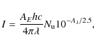
|
(1) |
where
|
(2) |
Standard interstellar extinction laws can be used to convert
![\begin{figure}
\par\includegraphics[width=9cm]{13828fg4.ps}
\end{figure}](/articles/aa/full_html/2010/09/aa13828-09/img63.png)
|
Figure 4:
K-band spectrum of the strongly H2 emitting region southeast of T Tau S at (0
|
| Open with DEXTER | |
In our data, two sets of lines share the same upper level. The v=1-0 S(1) and the v=1-0 Q(3) lines both arise from the v=1, J=3 level and the v=1-0 S(0) and the v=1-0 Q(2) lines both arise from the v=1, J=2 level. The Q-branch
is located in a spectral region where atmospheric correction is known
to be difficult, but by careful inspection of the corrected and the
uncorrected spectrum in the
![]() m interval, we find that the telluric absorption lines located in the continuum between the H2
lines are very well removed. That is, the continuum is featureless as
it should be with no or a few, weak traces of telluric lines after the
correction. We
assume that the correction for atmospheric absorption at the position
of H2lines is equally good and conclude that in these data the derived line flux is
not heavily biased by absorption. However, the atmospheric correction does
introduce an uncertainty to the derived line flux which we estimate to be
m interval, we find that the telluric absorption lines located in the continuum between the H2
lines are very well removed. That is, the continuum is featureless as
it should be with no or a few, weak traces of telluric lines after the
correction. We
assume that the correction for atmospheric absorption at the position
of H2lines is equally good and conclude that in these data the derived line flux is
not heavily biased by absorption. However, the atmospheric correction does
introduce an uncertainty to the derived line flux which we estimate to be ![]() 10%, but as this is generally smaller than the formal
uncertainty of the line flux we choose to ignore it.
10%, but as this is generally smaller than the formal
uncertainty of the line flux we choose to ignore it.
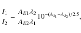
The visual extinction AV is estimated as
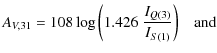
|
(3) | ||
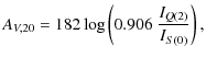
|
(4) |
where we have used the Einstein A coefficients from Turner et al. (1977).
Table 2: Line emission (in 10-2 erg s-1 cm-2 sr-1), radial velocity with respect to the rest velocity of T Tau Sa, tangential velocity, inclination angle, excitation temperature and size of the seven regions marked in Fig. 3.
In Fig. 5 we plot AV,31 vs. AV,20 for all spatial
points in the 25 mas data. The two estimates of the extinction do not agree very well. The majority of points lie
far from the
AV,31 = AV,20 line. While values of AV,31 are found
in the interval between 0 and 30, the AV,20 values show a much larger
spread ranging from -60 to 60. The large spread and the unphysical
negative values reflects the fact that the v=1-0 S(0) and the
v=1-0 Q(2) lines are much weaker than the v=1-0 S(1) and the
v=1-0 Q(3) lines and are therefore associated with much larger relative
uncertainty. For both AV,31 and AV,20 we calculated the AVinterval that is spanned when the flux of the lines is allowed to vary ![]()
![]() .
This analysis showed
three things: i) within the uncertainty, the AV,20 value is
always consistent with being positive; ii) for all pixels the AV,31 interval is smaller than the AV,20 interval and the AV,31 interval is always contained within the AV,20 interval; iii) even the AV,31 value, which is derived from two of the strongest H2 lines, spans a large range of values. The interval varies from
AV,31 =[0,15] in strongly emitting regions,
where the relative uncertainty on the line flux is typically 10%,
to [-30,80] in weak regions where the relative uncertainty is as high
as
.
This analysis showed
three things: i) within the uncertainty, the AV,20 value is
always consistent with being positive; ii) for all pixels the AV,31 interval is smaller than the AV,20 interval and the AV,31 interval is always contained within the AV,20 interval; iii) even the AV,31 value, which is derived from two of the strongest H2 lines, spans a large range of values. The interval varies from
AV,31 =[0,15] in strongly emitting regions,
where the relative uncertainty on the line flux is typically 10%,
to [-30,80] in weak regions where the relative uncertainty is as high
as ![]()
![]() .
For AV,20 the interval is typically
AV,20=[-15,65] in strongly emitting regions.
.
For AV,20 the interval is typically
AV,20=[-15,65] in strongly emitting regions.
![\begin{figure}
\par\includegraphics[width=9cm]{13828fg5.ps}
\end{figure}](/articles/aa/full_html/2010/09/aa13828-09/img70.png)
|
Figure 5: AV,31 vs AV,20 calculated for each spatial point in the 25 mas data. The solid line represents AV,31 = AV,20. |
| Open with DEXTER | |
This analysis shows that the derivation of extinction from line ratios is highly dependent on high signal-to-noise and high accuracy of flux determination. Our results clearly demonstrate the difficulty in obtaining reliable estimates of the extinction. Even a modest flux uncertainty of 10% results in a large uncertainty of the extinction value.
With this in mind, we use the AV values derived from the strongest lines, that is AV,31, as the best estimate of the extinction towards T Tau. Maps of AV,31 are shown in Fig. 6 and comparison with the contours of H2 brightness gives an impression of the uncertainty, keeping the above mentioned uncertainty limits in mind. Due to the large uncertainty in the values of AV we have not corrected the H2 line flux for extinction in any line.
Even though the absolute values of the extinction are highly uncertain, there
is reason to believe that the variations in AV are real. Variations of 15 mag AV are found in regions with the same v=1-0 S(1) brightness level. This means that AV is not correlated with H2 line brightness.
Furthermore, the overlapping regions in the 100 mas and 25 mas map in Fig. 6 show the same AVstructure around T Tau S. In addition, our 100 mas pixel scale image
(Fig. 6 left) agrees very well with the recently published
extinction map of Beck et al. (2008). In the 100 mas image (Fig. 6left)
the obscuring material between the north and south components is seen
to be part of a filament that continues to the east of T Tau.
South
of T Tau S, the extinction is lower by
![]() .
If the AV variations are real it implies that the circumstellar material is very clumpy. For a discussion of the implications see
Sect. 4.
.
If the AV variations are real it implies that the circumstellar material is very clumpy. For a discussion of the implications see
Sect. 4.
3.2.2 The  -0 S(1) /
  -1 S(1) line ratio
Near-infrared rovibrational emission lines from H2 arise in a number of physical processes, the most common of which are shock excitation and ultraviolet fluorescence. Line ratios of different H2 lines can be used to discriminate between these two mechanisms. The excitation mechanism at play is most clearly distinguished by comparing the emission in the v=1-0 to the emission in the v=2-1 vibrational band. Fluorescence results in stronger excitation to the high energy band than shock excitation. Here, we use the v=2-1 S(1) line as a representative for the emission in the v=2-1 band.
![\begin{figure}
\par\includegraphics[width=17.5cm,clip]{13828fg6.ps}
\end{figure}](/articles/aa/full_html/2010/09/aa13828-09/img71.png)
|
Figure 6:
Maps of extinction. The estimate AV,31 is shown for the 100 mas ( left) and 25 mas ( right) pixel scale. The colourbars indicate the magnitude of AV. Only regions in which the H2 v=1-0 S(1) line is detected at a 8 |
| Open with DEXTER | |
![\begin{figure}
\par\includegraphics[width=17.5cm,clip]{13828fg7.ps}
\vspace*{-2mm}
\end{figure}](/articles/aa/full_html/2010/09/aa13828-09/img72.png)
|
Figure 7:
H2 v=2-1 S(1) brightness in erg s-1 cm-2 sr-1. Left: 100 mas pixel scale, right: 25 mas pixel scale. Contours outline the v=1-0 S(1)
brightness. Only regions in which the v=2-1 S(1) line is detected at a 2 |
| Open with DEXTER | |
![\begin{figure}
\par\includegraphics[width=17cm]{13828fg8.ps}
\end{figure}](/articles/aa/full_html/2010/09/aa13828-09/img73.png)
|
Figure 8:
The ratio of H2 v=1-0 S(1) to v=2-1 S(1) line emission. Left: 100 mas pixel scale, right: 25 mas pixel scale. Contours outline the v=1-0 S(1) brightness. Only regions in
which the v=2-1 S(1) line is detected at a 2 |
| Open with DEXTER | |
Figure 7 shows the distribution of the v=2-1 S(1) line together with contours of the v=1-0 S(1) line. The v=2-1 S(1) emission is only detected around T Tau S and in the NW knot (Fig. 7 left). The spatial distribution of the v=2-1 S(1) emission is not identical to that of the v=1-0 S(1) emission. This becomes clearer in the right-hand side of the figure which shows the distribution of the v=2-1 S(1) line in the 25 mas pixel scale data. Emission from the v=2-1 S(1) transition is only detected southwest and southeast of T Tau S. Surprisingly, no v=2-1 S(1) emission is found northwest of the southern binary, even though the v=1-0 S(1) emission is strong in that region. Figure 8 shows the corresponding v=1-0 S(1)/v=2-1 S(1) line ratio map.
The different distribution of v=1-0 S(1) and v=2-1 S(1) emission results in a high variability in the line ratio. In Fig. 8 right, the lowest value of ![]() 8 is found southwest and southeast of T Tau S and is coincident with peaks in the v=1-0 S(1) emission. Closer to T Tau S and northwest of the binary, very little v=2-1 S(1) emission is detected and the line ratio reaches values of
8 is found southwest and southeast of T Tau S and is coincident with peaks in the v=1-0 S(1) emission. Closer to T Tau S and northwest of the binary, very little v=2-1 S(1) emission is detected and the line ratio reaches values of ![]() 15-20. A particular noteworthy feature is the flow at (-0
15-20. A particular noteworthy feature is the flow at (-0
![]() 1,-1
1,-1
![]() 0) (labelled
1a/1b in Fig. 3) which in the v=1-0 S(1) line appears to be one coherent entity with the shape of a horseshoe. In the v=2-1 S(1) line, the western side of the horseshoe (1b) closest to
T Tau S is weaker than the eastern side (1a) and in the line ratio map
there is no evidence of a horseshoe shape. The horseshoe could therefore
be the result of two flows instead of a single coherent flow.
0) (labelled
1a/1b in Fig. 3) which in the v=1-0 S(1) line appears to be one coherent entity with the shape of a horseshoe. In the v=2-1 S(1) line, the western side of the horseshoe (1b) closest to
T Tau S is weaker than the eastern side (1a) and in the line ratio map
there is no evidence of a horseshoe shape. The horseshoe could therefore
be the result of two flows instead of a single coherent flow.
The strength of the line emission from all the detected H2 lines in the
K-band extracted from the seven distinct emission features marked in Fig. 3 is listed in Table 2. In all seven regions the v=1-0 S(1)/v = 2-1 S(1)
line ratio is larger than 10. These values are only compatible
with shock excitation, since fluorescence produces values of ![]() 2 (Black & van Dishoeck 1987).
In the following sections, we work with the hypothesis that all - or at
least most - of the observed emission is caused by shocks.
2 (Black & van Dishoeck 1987).
In the following sections, we work with the hypothesis that all - or at
least most - of the observed emission is caused by shocks.
3.2.3 Excitation temperature
In the case of shock excitation, a super-Alfvenic shock wave rapidly heats the gas to temperatures of >1000 K. The temperature reached depends on the type of shock (J-shock or C-shock) as well as the shock velocity and the pre-shock conditions in the medium (Kristensen et al. 2007).
Using the line strengths of all available H2 lines,
we calculate the
excitation temperature in every spatial pixel. The excitation
temperature is the temperature that reproduces the observed line
ratios, assuming local
thermodynamic equilibrium, LTE. In LTE conditions, the column density
of level (v,J) is
| (5) |
where
|
(6) |
In Fig. 9, we plot
The line ratios in Fig. 9
are well represented within the uncertainties by a single linear fit
with an excitation temperature of 1990 K. The only exception is
the v=1-0 S(3) line which lies significantly
displaced from the linear fit. We ascribe this to poor correction for telluric
absorption in the 1.95 ![]() m spectral region and ignore the v=1-0 S(3) line in all further analysis. Note that the derived column densities of the Q-branch lines (Fig. 9) agree within the uncertainties with the column densities of the corresponding S-branch lines which share the same upper level. This is very comforting and supports our earlier
conclusion that the Q-branch is not significantly affected by errors in the correction for atmospheric absorption. Note also that no correction for
extinction has been applied to the line strengths. However, since all lines
lie in the K-band, any differential effect of extinction would be small,
m spectral region and ignore the v=1-0 S(3) line in all further analysis. Note that the derived column densities of the Q-branch lines (Fig. 9) agree within the uncertainties with the column densities of the corresponding S-branch lines which share the same upper level. This is very comforting and supports our earlier
conclusion that the Q-branch is not significantly affected by errors in the correction for atmospheric absorption. Note also that no correction for
extinction has been applied to the line strengths. However, since all lines
lie in the K-band, any differential effect of extinction would be small,
![]() from 2.0
from 2.0 ![]() m to 2.4
m to 2.4 ![]() m.
This is demonstrated in Fig. 9 where the column densities of
both uncorrected and dereddened data are plotted. The dereddening corresponds
to
m.
This is demonstrated in Fig. 9 where the column densities of
both uncorrected and dereddened data are plotted. The dereddening corresponds
to
![]() ,
which is the measured extinction in the emission region 2 (Fig. 6).
Dereddening causes small changes in the column densities which shifts
the fit towards higher temperatures. The temperature shift is well
within the uncertainty of the fit to the uncorrected data, however.
,
which is the measured extinction in the emission region 2 (Fig. 6).
Dereddening causes small changes in the column densities which shifts
the fit towards higher temperatures. The temperature shift is well
within the uncertainty of the fit to the uncorrected data, however.
![\begin{figure}
\par\includegraphics[width=9cm]{13828fg9.ps}
\end{figure}](/articles/aa/full_html/2010/09/aa13828-09/img80.png)
|
Figure 9:
Excitation diagram of the H2 emitting region
southeast of T Tau S at (0
|
| Open with DEXTER | |
The excitation temperature has been derived in all
spatial pixels, producing a map of excitation temperature
(Fig. 10). Only lines which are
detected at a >2![]() level are included in the fit.
This means that for the majority of spatial positions, only the S(1) line from
the v=2-1 band is included in the fit, since most of the other lines
from this band are weak and are rejected in the fit.
level are included in the fit.
This means that for the majority of spatial positions, only the S(1) line from
the v=2-1 band is included in the fit, since most of the other lines
from this band are weak and are rejected in the fit.
![\begin{figure}
\par\includegraphics[width=17cm]{13828f10.ps}
\end{figure}](/articles/aa/full_html/2010/09/aa13828-09/img81.png)
|
Figure 10:
Maps of excitation temperature. Left: 100 mas pixel scale, right: 25 mas pixel scale. The colourbars indicate the temperature in Kelvin. Only regions in which the v=2-1 S(1) line is detected at a 2 |
| Open with DEXTER | |
From Fig. 10, it is clear that the local peaks in H2 v=1-0 S(1) emission are associated with a large range of excitation temperatures.
The excitation temperature in the emission peaks at (0
![]() 35, -0
35, -0
![]() 65) and
(0
65) and
(0
![]() 3,-0
3,-0
![]() 4) (labelled 4 and 5 in Fig. 3) is
approximately 1300 K, while it is roughly 2100 K in
the peak at (-0
4) (labelled 4 and 5 in Fig. 3) is
approximately 1300 K, while it is roughly 2100 K in
the peak at (-0
![]() 02,-1
02,-1
![]() 15) (2 in Fig. 3). The cooler
regions are generally associated with more extinction than the warmer regions, but
although dereddening of the H2 lines would result in higher temperatures,
it is not sufficient to explain the temperature differences. The
difference in excitation temperature is real and indicates that the excitation
conditions of molecular hydrogen are not the same throughout the region.
15) (2 in Fig. 3). The cooler
regions are generally associated with more extinction than the warmer regions, but
although dereddening of the H2 lines would result in higher temperatures,
it is not sufficient to explain the temperature differences. The
difference in excitation temperature is real and indicates that the excitation
conditions of molecular hydrogen are not the same throughout the region.
3.2.4 Radial velocity
![\begin{figure}
\par\includegraphics[width=17cm]{13828f11.ps}
\end{figure}](/articles/aa/full_html/2010/09/aa13828-09/img82.png)
|
Figure 11:
Maps of radial velocity. Left: 100 mas pixel scale, right: 25 pixel scale mas. The colourbars indicate velocity in km s-1 with respect to the rest velocity of T Tau Sa of 22.0 km s-1. Contours outline the v=1-0 S(1) line brightness and only regions in which the v=1-0 S(1) line is detected at a 3 |
| Open with DEXTER | |
The radial velocity of H2 emitting gas has been calculated using the v=1-0 S(1) line at 2.12 ![]() m. Although SINFONI only has a spectral resolution
of
m. Although SINFONI only has a spectral resolution
of ![]() 75 km s-1 in the K-band, it is possible to determine the peak
position of the lines with much higher accuracy through line fitting. We have
derived the radial velocity corresponding to every H2 emitting position by
fitting a Gaussian profile to the unresolved line profiles on a pixel by pixel
basis and the velocity is found from the fitted peak position,
75 km s-1 in the K-band, it is possible to determine the peak
position of the lines with much higher accuracy through line fitting. We have
derived the radial velocity corresponding to every H2 emitting position by
fitting a Gaussian profile to the unresolved line profiles on a pixel by pixel
basis and the velocity is found from the fitted peak position, ![]() (see Sect. 3.2).
In our data, we do not find multiple peaks in the
spectral profiles. If more than one kinematic component should be
present in the line-of-sight, the multiple peaks in the spectrum are
smoothed by the spectral profile of SINFONI to the point where the
individual
peaks are indistinguishable. The derived radial velocity effectively
corresponds to the centroid velocity. The radial velocities have been
corrected for the
Earth's motion around the Sun at the time of observations. All
velocities are quoted as local velocities with respect to the
rest velocity of T Tau Sa of +22.0 km s-1 (Duchêne et al. 2005).
For reference, the heliocentric radial velocity
of T Tau Sb is +21.1 km s-1(Duchêne et al. 2005), while the radial velocity of T Tau N is +19.1 km s-1(Hartmann et al. 1986). In regions of the 25 mas pixel scale image with strong
signal and a high
signal-to-noise ratio, the estimated uncertainty from the fit,
(see Sect. 3.2).
In our data, we do not find multiple peaks in the
spectral profiles. If more than one kinematic component should be
present in the line-of-sight, the multiple peaks in the spectrum are
smoothed by the spectral profile of SINFONI to the point where the
individual
peaks are indistinguishable. The derived radial velocity effectively
corresponds to the centroid velocity. The radial velocities have been
corrected for the
Earth's motion around the Sun at the time of observations. All
velocities are quoted as local velocities with respect to the
rest velocity of T Tau Sa of +22.0 km s-1 (Duchêne et al. 2005).
For reference, the heliocentric radial velocity
of T Tau Sb is +21.1 km s-1(Duchêne et al. 2005), while the radial velocity of T Tau N is +19.1 km s-1(Hartmann et al. 1986). In regions of the 25 mas pixel scale image with strong
signal and a high
signal-to-noise ratio, the estimated uncertainty from the fit,
![]() ,
is on the order of 3-4 km s-1. In regions with weaker
emission the uncertainty is larger and may be as large as 20 km s-1.
For the 100 mas pixel size data, the typical uncertainty is
,
is on the order of 3-4 km s-1. In regions with weaker
emission the uncertainty is larger and may be as large as 20 km s-1.
For the 100 mas pixel size data, the typical uncertainty is ![]() 10 km s-1 in strong emission regions and up to 50 km s-1
in weak emission regions. The larger uncertainty in the 100 mas
pixel size data is due to lower signal-to-noise ratio than in the
25 mas data.
10 km s-1 in strong emission regions and up to 50 km s-1
in weak emission regions. The larger uncertainty in the 100 mas
pixel size data is due to lower signal-to-noise ratio than in the
25 mas data.
The velocity field appears in Fig. 11.
In the left hand side of Fig. 11, we see that the radial velocities
in the immediate surroundings of T Tau N are ![]() -2 km s-1, that is,
almost at rest in the rest frame of T Tau N. The gas around T Tau N is
associated with a nearly face-on circumstellar disk
(Gustafsson et al. 2008). South of T Tau N, the velocity of the gas is
-2 km s-1, that is,
almost at rest in the rest frame of T Tau N. The gas around T Tau N is
associated with a nearly face-on circumstellar disk
(Gustafsson et al. 2008). South of T Tau N, the velocity of the gas is ![]() -22 km s-1 and the velocity of
the NW filament is
-22 km s-1 and the velocity of
the NW filament is ![]() -7 km s-1. The measured velocities are
consistent with the velocities recorded in Herbst et al. (1997) and
Duchêne et al. (2005), as well as the velocity gradient in the
southeast-northwest direction detected in Herbst et al. (1997).
-7 km s-1. The measured velocities are
consistent with the velocities recorded in Herbst et al. (1997) and
Duchêne et al. (2005), as well as the velocity gradient in the
southeast-northwest direction detected in Herbst et al. (1997).
From the close-up (25 mas pixel scale data - right hand
side in figure), we find that the H2 blobs southeast and southwest of T Tau S are ![]() 20 km s-1
blue-shifted with respect to the stars. There seems to be a velocity
gradient with increasing velocity from the southeast to the northwest
of T Tau S. The northwest
corner is however still slightly blue-shifted with respect to the
stars. The horseshoe-shaped emission region southeast of
T Tau S (1a/1b in
Fig. 3) shows two distinct
velocity regions. The eastern most side (1a) has the highest velocity of
20 km s-1
blue-shifted with respect to the stars. There seems to be a velocity
gradient with increasing velocity from the southeast to the northwest
of T Tau S. The northwest
corner is however still slightly blue-shifted with respect to the
stars. The horseshoe-shaped emission region southeast of
T Tau S (1a/1b in
Fig. 3) shows two distinct
velocity regions. The eastern most side (1a) has the highest velocity of ![]() -22 km s-1 while the western side (1b) shows significantly lower velocities of
-22 km s-1 while the western side (1b) shows significantly lower velocities of ![]() -19 km s-1. This again argues
that the horseshoe-shaped emission feature is the result of two individual
shocks, as suggested in Sect. 3.2.2 based on the distribution
of the v=2-1 S(1) emission. The radial velocities of the seven flows marked in Fig. 3 are listed in Table 2.
-19 km s-1. This again argues
that the horseshoe-shaped emission feature is the result of two individual
shocks, as suggested in Sect. 3.2.2 based on the distribution
of the v=2-1 S(1) emission. The radial velocities of the seven flows marked in Fig. 3 are listed in Table 2.
![\begin{figure}
\par\includegraphics[width=17cm]{13828f12.ps}
\end{figure}](/articles/aa/full_html/2010/09/aa13828-09/img85.png)
|
Figure 12: H2 v=1-0 S(1) emission from December 2002 (colours, Herbst et al. 2007) and November 2004 (contours, our data). The data are aligned on T Tau Sa both in the large field of view image ( left) and in the small field of view ( right). The labeling of the flows of Herbst et al. (2007) is displayed in the large field of view for reference. |
| Open with DEXTER | |
In the immediate vicinity of T Tau Sb (at (0
![]() 2, -0
2, -0
![]() 7), labelled ``disk'' in Fig. 11) there is an elongated feature with velocities close to the velocity of the stars. The uncertainties
on the velocities of this feature are
7), labelled ``disk'' in Fig. 11) there is an elongated feature with velocities close to the velocity of the stars. The uncertainties
on the velocities of this feature are ![]() 10 km s-1, which are large
compared to the span of velocities in the surroundings (
10 km s-1, which are large
compared to the span of velocities in the surroundings (![]() 20 km s-1). However, the
feature shows up in each individual exposure with different nodding offsets
and it is also clearly distinguishable in the 100 mas data (left hand side of
Fig. 11). Thus, little doubt can remain that this feature is real
and we speculate that it might be related to a rotating circumstellar or
circumbinary disk within the T Tau S system.
20 km s-1). However, the
feature shows up in each individual exposure with different nodding offsets
and it is also clearly distinguishable in the 100 mas data (left hand side of
Fig. 11). Thus, little doubt can remain that this feature is real
and we speculate that it might be related to a rotating circumstellar or
circumbinary disk within the T Tau S system.
The velocities measured here are consistent with the results from
Duchêne et al. (2005), who found that the emission became increasingly
blue-shifted moving away from the southern binary in the east-west direction
until a blue-shift of 10 km s-1 was reached ![]()
![]() away on either side of the stars. The velocity map is also consistent with that of Beck et al. (2008).
away on either side of the stars. The velocity map is also consistent with that of Beck et al. (2008).
3.2.5 Proper motions
Recently, Herbst et al. (2007) published high spatial resolution images of H2in the T Tau system. Their data were obtained with NACO on the ESO-VLT on the
nights of December 14-15 2002.
By a direct comparison where we plot the data of Herbst et al. (2007)
together with our data (Fig. 12) we can see how the H2 emission has evolved in the central region of T Tau on a
timescale of ![]() 2 years. The data are aligned on T Tau Sa, which is the most massive star in the triple system (Köhler 2008).
2 years. The data are aligned on T Tau Sa, which is the most massive star in the triple system (Köhler 2008).
From the large field of view, it seems that the NW emission knot, of which only the southern tip is visible in our data, has remained in the same position during the time-span of 2 years. The outline of the main emission region around T Tau S is also roughly the same in the two epochs, although the contours suggest that the southern part has expanded. No proper motions are detectable in these data for the H2 flows NW and W of T Tau S labelled C1 and C2 in Herbst et al. (2007) (flow called bow and nr 5+6 in Fig. 3). The proper motions of the flows south of T Tau S, labelled C3 and C4 in Herbst et al. (2007) are discussed below.
A more detailed picture is found in the smaller field. The strongly emitting
peak or complex of peaks to the northwest of T Tau S (4, 5, 6 in
Fig. 3, C2 in Herbst et al. 2007) does not seem to have
changed position. In contrast, the southwestern peak (3 in
Fig. 3, C3 in Herbst et al. 2007), which resembles a
bow shock originating in one of the T Tau S stellar components, has moved away from the stars by ![]() 0
0
![]() 09, corresponding to an average velocity of
09, corresponding to an average velocity of ![]() 32 km s-1. Using the radial velocity of
32 km s-1. Using the radial velocity of ![]() 17 km s-1 with respect to T Tau Sa/Sb found in this bow shock (Fig. 11) we derive a 3D velocity of
17 km s-1 with respect to T Tau Sa/Sb found in this bow shock (Fig. 11) we derive a 3D velocity of ![]() 36 km s-1 and an inclination of the flow to the line of sight of
36 km s-1 and an inclination of the flow to the line of sight of ![]()
![]() .
The direction of the proper motion indicates that this bow shock comes from T Tau Sb.
.
The direction of the proper motion indicates that this bow shock comes from T Tau Sb.
The peak which appeared southeast at (-0
![]() 05,-0
05,-0
![]() 95) in
2002 (C4 in Herbst et al. 2007)
has clearly developed, but it is unclear with
which blob in the 2004 data the 2002 blob should be associated. It
could have developed into either of the two southeastern blobs at (0
95) in
2002 (C4 in Herbst et al. 2007)
has clearly developed, but it is unclear with
which blob in the 2004 data the 2002 blob should be associated. It
could have developed into either of the two southeastern blobs at (0
![]() 05, -1
05, -1
![]() 2) and (-0
2) and (-0
![]() 1,-1
1,-1
![]() 05) (1a/1b and 2 in Fig. 3). As
mentioned above, the horseshoe-shaped flow at (-0
05) (1a/1b and 2 in Fig. 3). As
mentioned above, the horseshoe-shaped flow at (-0
![]() 1, -1
1, -1
![]() 05) is most
likely made up of two distinct flows. Thus, the 2002 southeast blob could have
developed into any of the three flows in 2004. Judging from the morphology and
the implied direction of the proper motions, we consider it most likely that
the 2002 blob has developed into the eastern flow of the horseshoe (1a). This
flow
would then originate in T Tau Sa and from the proper motion of 0
05) is most
likely made up of two distinct flows. Thus, the 2002 southeast blob could have
developed into any of the three flows in 2004. Judging from the morphology and
the implied direction of the proper motions, we consider it most likely that
the 2002 blob has developed into the eastern flow of the horseshoe (1a). This
flow
would then originate in T Tau Sa and from the proper motion of 0
![]() 15 we
derive a space velocity of
15 we
derive a space velocity of ![]() 53 km s-1. Together with the radial
velocity of
53 km s-1. Together with the radial
velocity of ![]() 22 km s-1 with respect to T Tau Sa the 3D velocity is
then
22 km s-1 with respect to T Tau Sa the 3D velocity is
then ![]() 57 km s-1 and the inclination of the flow is
57 km s-1 and the inclination of the flow is ![]()
![]() .
.
3.3 Lines in J-band
Only two extended emission lines were detected in the J-band, namely
Pa![]() at 1.282
at 1.282 ![]() m and [Fe II] at 1.257
m and [Fe II] at 1.257 ![]() m. The fact that Pa
m. The fact that Pa![]() is
observed to be spatially extended is most likely due to scattering of
light from the stars - mainly T Tau N - and not local
emission. Further evidence favouring this conclusion is given by the
fact that the
Pa
is
observed to be spatially extended is most likely due to scattering of
light from the stars - mainly T Tau N - and not local
emission. Further evidence favouring this conclusion is given by the
fact that the
Pa![]() line to continuum ratio is more or less constant over the whole field of view. The extent of the continuum emission and thus Pa
line to continuum ratio is more or less constant over the whole field of view. The extent of the continuum emission and thus Pa![]() can be seen in Fig. 1.
can be seen in Fig. 1.
![\begin{figure}
\par\includegraphics[width=9cm]{13828f13.ps}
\end{figure}](/articles/aa/full_html/2010/09/aa13828-09/img89.png)
|
Figure 13:
Small field of view. [Fe II] emission at 1.257 |
| Open with DEXTER | |
Table 3: Best fit 1D shock models to the seven flows in Fig. 3.
The [Fe II] emission shows a different spatial distribution (Fig. 13)
to that of Pa![]() with a region of very strong emission in the northern
part of the field between T Tau S and T Tau N,
extending to the west. [Fe II] emission must therefore be emitted
locally in the ambient
gas. To the southeast of T Tau S there is a strong
[Fe II] emission region as well. It is also clear that
[Fe II] and H2 emission are
not spatially coincident. In the region between T Tau N and T Tau S both the
H2 and the [Fe II] emission are strong, whereas we detect very little
[Fe II] emission from the H2 flow to the southwest of T Tau S (flow nr 3).
To the southeast of T Tau S both H2 and Fe emission is detected but the peak
of the [Fe II] emission is spatially offset from that of the H2 and is found
closer to the stars. The different spatial distributions of H2 and Fe emission is to be expected since [Fe II] emission is mainly produced in J-type shocks where H2 is dissociated and the H2 emission is consequently low.
with a region of very strong emission in the northern
part of the field between T Tau S and T Tau N,
extending to the west. [Fe II] emission must therefore be emitted
locally in the ambient
gas. To the southeast of T Tau S there is a strong
[Fe II] emission region as well. It is also clear that
[Fe II] and H2 emission are
not spatially coincident. In the region between T Tau N and T Tau S both the
H2 and the [Fe II] emission are strong, whereas we detect very little
[Fe II] emission from the H2 flow to the southwest of T Tau S (flow nr 3).
To the southeast of T Tau S both H2 and Fe emission is detected but the peak
of the [Fe II] emission is spatially offset from that of the H2 and is found
closer to the stars. The different spatial distributions of H2 and Fe emission is to be expected since [Fe II] emission is mainly produced in J-type shocks where H2 is dissociated and the H2 emission is consequently low.
4 Discussion
We now use the measurements of the H2 emission to model the physical conditions in the environment of T Tau. H2 emission offset from the central source is usually associated with shocks produced by outflows and the excitation pattern of H2 is very sensitive to the shock conditions. We seek to reproduce the H2 brightness of the seven emission regions given in Table 2 with state-of-the-art planar shock models in order to estimate the underlying shock parameters.
First, we note that the size of the observed shocks constrains the density of
the pre-shock gas. In a
![]() cm-3 medium, the shock width
is
cm-3 medium, the shock width
is ![]() 100 AU (see Fig. 8 in Kristensen et al. 2007), that is, much
larger than the size of the observed shocks. On the other hand, in a
100 AU (see Fig. 8 in Kristensen et al. 2007), that is, much
larger than the size of the observed shocks. On the other hand, in a
![]() cm-3 medium the shock width is a few AU, which is very narrow
compared to what we observe even if projection effects are considered.
Thus, the pre-shock densities are most likely to be found in the
cm-3 medium the shock width is a few AU, which is very narrow
compared to what we observe even if projection effects are considered.
Thus, the pre-shock densities are most likely to be found in the
![]() -
-
![]() cm-3 range.
cm-3 range.
We use the grid of planar
C-shocks described in Kristensen et al. (2007) and a ![]() analysis to find
the shock that best matches the observed line emission of the 12 H2 lines.
The grid in Kristensen et al. (2007) was calculated using the shock code described
in Flower & Pineau des Forêts (2003) and references therein, in which a large chemical reaction
network with 1065 processes involving 136 species is included.
The range of input parameters in the shock grid is as follows:
analysis to find
the shock that best matches the observed line emission of the 12 H2 lines.
The grid in Kristensen et al. (2007) was calculated using the shock code described
in Flower & Pineau des Forêts (2003) and references therein, in which a large chemical reaction
network with 1065 processes involving 136 species is included.
The range of input parameters in the shock grid is as follows:
- pre-shock density, nH:
 ,
105,
,
105,
 ,
106,
,
106,
 ,
107 cm-3;
,
107 cm-3;
- shock velocity: 10-50 km s-1, step size of 1 km s-1;
- transverse magnetic flux density,
 G with the
scaling factor
b= 0.5-10, step size of 0.5;
G with the
scaling factor
b= 0.5-10, step size of 0.5;
- initial ortho/para ratio: 3.0.
The modelling of the flows in the vicinity of T Tau shows that the ambient
material is very dense with a pre-shock density of ![]()
![]() cm-3. All flows are consistent with being excited by a shock wave
moving at a speed of 17-24 km s-1 in a
B=0.35-0.70 mG medium.
These shock velocities are considerable lower than the 3D velocities of flow
1a (57 km s-1) and 3 (36 km s-1) derived in Sect. 3.2.5
from the radial velocities and proper motions. One way to reconcile
these
seemingly contradictory facts is if the shocked medium has been
accelerated
prior to the arrival of the shock wave. This could have been done by a
previous passing shock wave that simultaneously would have compressed
the gas. If this scenario is true, the velocity of the impinging
outflow is higher than the modelled shock velocity and at least as high
as the 3D velocity of the flows.
cm-3. All flows are consistent with being excited by a shock wave
moving at a speed of 17-24 km s-1 in a
B=0.35-0.70 mG medium.
These shock velocities are considerable lower than the 3D velocities of flow
1a (57 km s-1) and 3 (36 km s-1) derived in Sect. 3.2.5
from the radial velocities and proper motions. One way to reconcile
these
seemingly contradictory facts is if the shocked medium has been
accelerated
prior to the arrival of the shock wave. This could have been done by a
previous passing shock wave that simultaneously would have compressed
the gas. If this scenario is true, the velocity of the impinging
outflow is higher than the modelled shock velocity and at least as high
as the 3D velocity of the flows.
The complex outflow pattern with many arcs and filaments within 10
![]() of
the stars (Herbst et al. 1997) is also evidence of past episodic flows.
Further support of the idea that shock waves have previously crossed the region
is found in the short cooling times of the modelled shocks of a few years. The cooling time of a
shock is closely associated with the cooling distance and is therefore largely
set by the observed size of the emission region. Given the tight constraint the
observed shock width puts on the cooling time, it is certain that the flows we
see have not been detectable for more than a few years. Therefore, a succesive
generation of shocks seems
necessary in order to explain that the presence of
strong H2 emission in the inner 1
of
the stars (Herbst et al. 1997) is also evidence of past episodic flows.
Further support of the idea that shock waves have previously crossed the region
is found in the short cooling times of the modelled shocks of a few years. The cooling time of a
shock is closely associated with the cooling distance and is therefore largely
set by the observed size of the emission region. Given the tight constraint the
observed shock width puts on the cooling time, it is certain that the flows we
see have not been detectable for more than a few years. Therefore, a succesive
generation of shocks seems
necessary in order to explain that the presence of
strong H2 emission in the inner 1
![]() of T Tau S has been observed
for more than a decade (e.g. Herbst et al. 1996). With the recent high spatial
resolution data, it has for the first time become feasible to trace individual
flows, and with future follow up observations, these ideas can be fully tested.
of T Tau S has been observed
for more than a decade (e.g. Herbst et al. 1996). With the recent high spatial
resolution data, it has for the first time become feasible to trace individual
flows, and with future follow up observations, these ideas can be fully tested.
![\begin{figure}
\par\includegraphics[angle=0, width=16cm]{13828f14.eps}
\end{figure}](/articles/aa/full_html/2010/09/aa13828-09/img103.png)
|
Figure 14:
Overlay of the UV fluorescent H2 emission (contours) from Saucedo et al. (2003) on the H2 2.12 |
| Open with DEXTER | |
The modelling of the flows in T Tau shows that flow 1a and 1b can both - even
though treated independently - arise from a C-shock with the same
parameters. Perhaps they should not be attributed to two different shock waves afterall. 3D modelling of
shocks shows that a bow shock can create a horseshoe shaped emission morphology
like that of 1a/1b if the direction of the magnetic field is inclined with
respect to the propagation axis of the bow shock and the shock is moving at an
angle to the line-of-sight of ![]()
![]() (Fig. A.3
in Gustafsson et al. 2009). The radial velocity map of a shock with this geometry (Fig. 10 in Gustafsson et al. 2009) is also consistent with our observations
(Fig. 11). One side of the horseshoe displays significantly higher
blueshifted velocities than the other side.
(Fig. A.3
in Gustafsson et al. 2009). The radial velocity map of a shock with this geometry (Fig. 10 in Gustafsson et al. 2009) is also consistent with our observations
(Fig. 11). One side of the horseshoe displays significantly higher
blueshifted velocities than the other side.
The seven flows in the vicinity of T Tau S have all been successfully modelled with C-type shocks. In C-shocks the production of [Fe II] emission is very low and not sufficient to explain the observed [Fe II] brightness. Instead, the [Fe II] brightness indicates that J-type shocks in which [Fe II] emission is more readily produced surround the C-shocks. In the simplest possible geometry, where a bow shock is seen edge-on, J-shocks are usually found on the outside of C-shocks. At other inclinations the Fe emission from J-shocks may appear on the inside of the H2 emission produced by C-shocks (Gustafsson et al. 2009). This is indeed what we see to the southeast of T Tau S.
Saucedo et al. (2003) detected UV fluorescent H2 emission in two arcs south of T Tau S close to the 2.12 ![]() m flows (1a, 1b, 2) and in a lobe SW of T Tau N
coincident with the flows nr 5 and 6 here (Fig. 14).
There is a considerable spatial overlap between flourescent H2 and [Fe II]
emission (Fig. 14 right) and it is very plausible that the
J-shocks associated with the [Fe II] emission powers the flourescence as suggested in Saucedo et al. (2003). It is interesting that the northern lobe of fluorescent H2 emission is spatially coincident with our flows nr 5 and 6 where little or no emission
in the H2 v=2-1 S(1) line was detected. This led us to rule out
fluorescence as the excitation mechanism of the near-infrared H2 emission.
From the distribution of the near-infrared H2 emission, the UV H2fluorescence and the [Fe II] emission, we conclude that the near-infrared H2emission is dominated by excitation in C-shocks. Fluorescence also
contribute to the population of the H2 levels, but since it is powered by
J-shocks the associated excitation is overwhelmed by the much stronger
excitation from the C-shocks.
m flows (1a, 1b, 2) and in a lobe SW of T Tau N
coincident with the flows nr 5 and 6 here (Fig. 14).
There is a considerable spatial overlap between flourescent H2 and [Fe II]
emission (Fig. 14 right) and it is very plausible that the
J-shocks associated with the [Fe II] emission powers the flourescence as suggested in Saucedo et al. (2003). It is interesting that the northern lobe of fluorescent H2 emission is spatially coincident with our flows nr 5 and 6 where little or no emission
in the H2 v=2-1 S(1) line was detected. This led us to rule out
fluorescence as the excitation mechanism of the near-infrared H2 emission.
From the distribution of the near-infrared H2 emission, the UV H2fluorescence and the [Fe II] emission, we conclude that the near-infrared H2emission is dominated by excitation in C-shocks. Fluorescence also
contribute to the population of the H2 levels, but since it is powered by
J-shocks the associated excitation is overwhelmed by the much stronger
excitation from the C-shocks.
4.1 The origin of the flows
There are two clear outflow systems arising from the three stars in the T Tau system, but it has proven difficult to settle to which star each outflow should be assigned. There is an east-west jet ending in the Herbig-Haro object HH 155 (Bührke et al. 1986) which was assigned to T Tau N by Böhm & Solf (1994) and Solf & Böhm (1999) on the basis of position-velocity diagrams from long-slit spectra. In contrast, near-infrared observations of H2 led Herbst et al. (1996) to associate T Tau S with the east-west flow. In Herbst et al. (2007) the morphology of the H2 flows in the vicinity of T Tau S was interpreted as a bow shock (C1 in Herbst et al. (2007), named ``bow'' in Fig. 3) coming from T Tau S with bright, oblique shocks lining the flow channel (C2 and C3 in Herbst et al. (2007), flows number 3, 5, and 6 here). This would unambiguously identify T Tau S as the source of the east-west flow. This interpretation is however challenged by the proper motions of the H2 filaments derived in this paper. The proper motions show that the flow 3/C3 is moving in the southwest direction away from T Tau S whereas the flows 5+6/C2 and bow/C1 have not moved in the intermediate time period. It is difficult to see how such a flow pattern could arise in a single bow shock with limb brightened shocks in the wings. It is therefore more likely that the 3/C3 flow constitutes an independent outflow (the ``missing'' third outflow from the three stars?) and should not be associated with the C1 and 5+6/C2 flows. The proper motion shows that outflow 3 is coming from the southern binary with a preference for T Tau Sb. However, given the small separation of the binary, T Tau Sa cannot be ruled out as the source.
From the geometry of the outflows and the radial velocity we argue that the flows 1a/1b and 2 are the blue-shifted counterparts to the more red-shifted NW flow (Herbst et al. 1997). The flows 1a/1b and 2 are thus part of the southeast-northwest outflow called C-D in Böhm & Solf (1994). The proper motions pin-point the origin of the 1a/1b flow and thus the southeast-northwest outflow to the T Tau S binary. Radio emission at 6 cm in the southeast-northwest direction has also been found centered on T Tau S (Ray et al. 1997) and recently van Boekel et al. (2009) found bright [NeII] emission centered on T Tau S and extending to the NW filament. All this is further evidence favouring T Tau S as the driving source of the southeast-northwest outflow. However, as with the flow nr 3, there is an ambiguity between T Tau Sa and Sb.
Loinard et al. (2007a) identified the radio source
south of T Tau N with T Tau Sb and detected extended radio emission at 3.6 cm
from this source at position angle (PA)
![]() (or
(or
![]() ). The radio emission is presumably produced by the interaction of a stellar wind with
circumstellar material. The PA of flow 3 is
). The radio emission is presumably produced by the interaction of a stellar wind with
circumstellar material. The PA of flow 3 is
![]() with respect to T Tau Sb and is remarkably close to the PA of the radio emission.
We argue that the flow 3 originates in T Tau Sb and is one of the shocks
produced when the wind from the star impinges on the ambient gas.
with respect to T Tau Sb and is remarkably close to the PA of the radio emission.
We argue that the flow 3 originates in T Tau Sb and is one of the shocks
produced when the wind from the star impinges on the ambient gas.
Based on mid-infrared interferometry Ratzka et al. (2009) modelled the inclination
of the disk around T Tau Sa to be ![]()
![]() compared to
compared to
![]() for the disk around T Tau Sb. The inclination of the disk of
T Tau Sa fits very well with the inclination of the
southeast-northwest outflow of
for the disk around T Tau Sb. The inclination of the disk of
T Tau Sa fits very well with the inclination of the
southeast-northwest outflow of
![]() (Solf & Böhm 1999). We have used the proper motions and radial velocities to estimate the inclination of flow 1a. The inclination,
(Solf & Böhm 1999). We have used the proper motions and radial velocities to estimate the inclination of flow 1a. The inclination,
![]() is consistent with the
inclination of the southeast-northwest outflow.
This all seems to favour T Tau Sa as the source of the southeast-northwest
flow and T Tau Sb as the source of the ``new'' southwest outflow. The
inclination of flow 3 of
is consistent with the
inclination of the southeast-northwest outflow.
This all seems to favour T Tau Sa as the source of the southeast-northwest
flow and T Tau Sb as the source of the ``new'' southwest outflow. The
inclination of flow 3 of ![]()
![]() is larger than the inferred
inclination of the disk around T Tau Sb of
is larger than the inferred
inclination of the disk around T Tau Sb of
![]() (Ratzka et al. 2009) but
since both results are relatively uncertain the values are not irreconcilable.
(Ratzka et al. 2009) but
since both results are relatively uncertain the values are not irreconcilable.
Since the orbital period of the southern binary is only 21-28 years
(Duchêne et al. 2006; Köhler 2008) the position of the stellar components was
quite different when the exciting jets were launched than at the time of
observation. If we assume that the
velocity of the jets equals the derived space
velocity - 32 km s-1 and 53 km s-1 of flow 3 and 1a, respectively
(Sect. 3.2.5) - the exciting jets from T Tau Sa and T Tau Sb should
have been launched close to the periastron passage, namely between 1995 and
1999. In that period the position angle was ![]()
![]() (Köhler 2008). The star-jet association above is fully consistent with the
stellar positions at the time of launch. The extended structure 1a/1b/2,
consisting of short-lived emission regions, originating from a sequence of
outflows, might be the result of precession of the jet from T Tau Sa due to
the orbital motion of T Tau Sb. Thus, the H2 emission regions might
bear witness to the short orbital period of the binary.
(Köhler 2008). The star-jet association above is fully consistent with the
stellar positions at the time of launch. The extended structure 1a/1b/2,
consisting of short-lived emission regions, originating from a sequence of
outflows, might be the result of precession of the jet from T Tau Sa due to
the orbital motion of T Tau Sb. Thus, the H2 emission regions might
bear witness to the short orbital period of the binary.
If the southern binary drives the southeast-northwest and the southwest
outflow, T Tau N must be the driving source of the east-west flow, which in
our data are represented by flow 5+6 and the flow called ``bow''.
That is further supported by the presence of
extended radio emission at 2 cm from T Tau N at position angle
![]() or
or
![]() (Loinard et al. 2007a). The angle of the radio outflow is consistent with the PA from T Tau N to
``bow'' of
(Loinard et al. 2007a). The angle of the radio outflow is consistent with the PA from T Tau N to
``bow'' of ![]()
![]() .
Furthermore, the low (unmeasurable) tangential velocities in the flow
5+6 and ``bow'' indicate that the east-west flow is moving at a low
inclination to the line of sight. The inclination of T Tau N
is
.
Furthermore, the low (unmeasurable) tangential velocities in the flow
5+6 and ``bow'' indicate that the east-west flow is moving at a low
inclination to the line of sight. The inclination of T Tau N
is
![]() (Herbst et al. 1997) and the inclination of HH 155 which is believed to be the
working surface of the east-west jet is
(Herbst et al. 1997) and the inclination of HH 155 which is believed to be the
working surface of the east-west jet is
![]() (Eislöffel & Mundt 1998).
Our proposed solution to the enigma of the outflows in T Tauri is summarized
in Table 4.
The proposed association of stars and flow implies that all three disks are
misaligned and that three different stars
are driving the flows in the immediate vicinity of T Tau S. T Tau Sa drives
flow 1a/1b and 2, T Tau Sb drives flow nr 3 and T Tau N drives flow nr 5 and
6. With this association it is easily explained why all flows in a
(Eislöffel & Mundt 1998).
Our proposed solution to the enigma of the outflows in T Tauri is summarized
in Table 4.
The proposed association of stars and flow implies that all three disks are
misaligned and that three different stars
are driving the flows in the immediate vicinity of T Tau S. T Tau Sa drives
flow 1a/1b and 2, T Tau Sb drives flow nr 3 and T Tau N drives flow nr 5 and
6. With this association it is easily explained why all flows in a
![]() angle around T Tau S are blueshifted.
The misalignment of the three disks in T Tauri is quite puzzling. For a
detailed discussion of possible formation scenarios we refer to
Ratzka et al. (2009).
angle around T Tau S are blueshifted.
The misalignment of the three disks in T Tauri is quite puzzling. For a
detailed discussion of possible formation scenarios we refer to
Ratzka et al. (2009).
Table 4: Outflows and associated sources in T Tauri.
4.2 The nature of the obscuring material
From our extinction maps (Fig. 6)
it is evident that the extinction
is high in the immediate surroundings of T Tau S and in the
area between T Tau N and T Tau S. As mentioned
previously (Fig. 6 left) the obscuring material between
the north and south components is seen to be part of a
filament that continues to the east of T Tau. South
of T Tau S, the extinction is lower by
![]() .
The extinction close to T Tau N cannot be assessed due to the large amount of scattered light which
swamps the H2 lines. The extinction of
.
The extinction close to T Tau N cannot be assessed due to the large amount of scattered light which
swamps the H2 lines. The extinction of
![]() close to T Tau S is consistent with what previous authors find towards T Tau S (
AV = 17.4, van den Ancker et al. (1999);
AV = 5-27, Beck et al. 2004). The region of high extinction northeast of T Tau S may be associated with the 0
close to T Tau S is consistent with what previous authors find towards T Tau S (
AV = 17.4, van den Ancker et al. (1999);
AV = 5-27, Beck et al. 2004). The region of high extinction northeast of T Tau S may be associated with the 0
![]() 5
5 ![]() 0
0
![]() 64 structure of obscuring material observed by Walter et al. (2003). From our map, it is clear
that the northeast structure does not resemble a simple edge-on disk around T Tau Sa as suggested by Walter et al. (2003) or a circumbinary disk around both T Tau S components (Duchêne et al. 2005). Instead, we suggest that the obscuration is due to a
combination of a circumbinary disk around T Tau S, the circumstellar disk
around T Tau N (Gustafsson et al. 2008) and a long (>2
64 structure of obscuring material observed by Walter et al. (2003). From our map, it is clear
that the northeast structure does not resemble a simple edge-on disk around T Tau Sa as suggested by Walter et al. (2003) or a circumbinary disk around both T Tau S components (Duchêne et al. 2005). Instead, we suggest that the obscuration is due to a
combination of a circumbinary disk around T Tau S, the circumstellar disk
around T Tau N (Gustafsson et al. 2008) and a long (>2
![]() in the
east-west direction) dust filament between T Tau N and
T Tau S. A circumstellar disk around T Tau Sa may
also be present in order to explain the non-detection of this star at
wavelengths short-ward of 1.6
in the
east-west direction) dust filament between T Tau N and
T Tau S. A circumstellar disk around T Tau Sa may
also be present in order to explain the non-detection of this star at
wavelengths short-ward of 1.6 ![]() m.
The dust filament may be a result of the star-star interaction or it may be a foreground object.
m.
The dust filament may be a result of the star-star interaction or it may be a foreground object.
5 Summary
We have presented new high spatial resolution observations of T Tau in the
near-infrared. The integral field spectroscopic data obtained with SINFONI
enables us to trace the emission produced in shocks from outflows in 12 H2 rovibrational emission lines as well as the [Fe II] line at 1.257 ![]() m.
m.
H2 is detected everywhere within 2
![]() of T Tau N, with the strongest
emission concentrated around the southern binary T Tau S. A number of the
strongly emitting regions have a bow shock morphology. We have not detected
any H2 emission in the stellar components.
of T Tau N, with the strongest
emission concentrated around the southern binary T Tau S. A number of the
strongly emitting regions have a bow shock morphology. We have not detected
any H2 emission in the stellar components.
We have used four H2 lines - two pairs with the same upper energy level - to analyse the extinction around T Tau. The absolute values of AV are highly uncertain and relies on high accuracy of flux determination in the lines involved. The variations in AV are however uncorrelated with brightness and are believed to be real. The extinction is very high around T Tau S and in the region between T Tau S and N. The obscuring material seems to be part of a filament that stretches to the east of T Tau.
The v=1-0 S(1)/ v=2-1 S(1) line ratio is highly variable ranging from ![]() 8-20. The high values are incompatible with excitation by UV
fluorescence and indicates that all - or at least most - of the detected H2 emission arises in shocks.
8-20. The high values are incompatible with excitation by UV
fluorescence and indicates that all - or at least most - of the detected H2 emission arises in shocks.
We have derived the map of excitation temperature using all H2 lines which
are detected at a >2![]() level. The excitation temperature varies between 1200 K and
2600 K and there is a clear trend of increasing temperature at
increasing distance to the stars.
level. The excitation temperature varies between 1200 K and
2600 K and there is a clear trend of increasing temperature at
increasing distance to the stars.
The radial velocity of H2 emitting gas has been calculated from line fitting
to the v=1-0 S(1)
line. The radial velocities in the vicinity of T Tau N are
very close to the rest velocity of the star and are associated with a
nearly
face-on circumstellar disk (Gustafsson et al. 2008). The shocks southeast and
southwest of T Tau S are ![]() 20 km s-1 blueshifted with respect to the
stars, while the shocks northwest of T Tau S are
20 km s-1 blueshifted with respect to the
stars, while the shocks northwest of T Tau S are ![]() 7 km s-1blueshifted. All the shocked gas surrounding T Tau S is thus blueshifted.
7 km s-1blueshifted. All the shocked gas surrounding T Tau S is thus blueshifted.
Based on data taken two years prior to our observations (Herbst et al. 2007)
we have measured the proper motions of the observed shocks. These show that
the southwest flow is moving away from T Tau Sb with a speed of 36 km s-1at an inclination of ![]()
![]() .
The southeast flow is moving at a
higher speed of 57 km s-1 at an inclination of
.
The southeast flow is moving at a
higher speed of 57 km s-1 at an inclination of ![]()
![]() .
In
contrast, there are no detectable proper motions for the shocks northwest and
west of T Tau S, which suggests that they move at lower velocities or close to
the line of sight.
.
In
contrast, there are no detectable proper motions for the shocks northwest and
west of T Tau S, which suggests that they move at lower velocities or close to
the line of sight.
We have modelled seven individual flows in T Tau with state of the art C-shock
models. The modelling shows that the ambient medium in which the shocks
propagate is very dense with pre-shock densities of
![]() cm-3. All flows are consistent with being excited by a shock
wave at a speed of 17-24 km s-1 in a
B= 0.35-0.70 mG medium. The
inferred shock velocity is lower than the measured 3D velocity, which might
suggest that the gas around T Tau has been accelerated by an earlier
passing shock wave.
cm-3. All flows are consistent with being excited by a shock
wave at a speed of 17-24 km s-1 in a
B= 0.35-0.70 mG medium. The
inferred shock velocity is lower than the measured 3D velocity, which might
suggest that the gas around T Tau has been accelerated by an earlier
passing shock wave.
We detect strong [Fe II] emission northwest and south of T Tau S. The [Fe II] and H2 emission are not spatially coincident. [Fe II] is mainly produced in J-type shocks where H2 is dissociated. There is a strong overlap between the distribution of [Fe II] emission and UV flourescent H2 emission. The UV flourescence might be powered by J-shocks.
Based on the SINFONI data together with the proper motions we propose that outflows from all three stars in the T Tau system contribute to the H2emission in the immediate vicinity of T Tau S. T Tau N drives the shocks northwest of T Tau S and is associated with the east-west outflow. T Tau Sa drives the flows southeast of the southern binary and is the source of the southeast-northwest outflow. T Tau Sb is the origin of a previously undetected outflow in the southwest direction. The proposed association of stars and outflows implies that all three disks are misaligned.
AcknowledgementsPart of this paper was written during an extended visit to Aarhus University, Denmark. M.G. gratefully acknowledge the support of Aarhus University and MPIA in order to make this possible.
References
- Akeson, R. L., Koerner, D. W., & Jensen, E. L. N. 1998, ApJ, 505, 358 [NASA ADS] [CrossRef] [Google Scholar]
- Beck, T. L., Prato, L., & Simon, M. 2001, ApJ, 551, 1031 [NASA ADS] [CrossRef] [Google Scholar]
- Beck, T. L., Schaefer, G. H., Simon, M., et al. 2004, ApJ, 614, 235 [NASA ADS] [CrossRef] [Google Scholar]
- Beck, T. L., McGregor, P. J., Takami, M., et al. 2008, ApJ, 676, 472 [NASA ADS] [CrossRef] [Google Scholar]
- Bevington, P. 1969, Data reduction and Error Analysis for the Physical Sciences (New York: McGraw-Hill) [Google Scholar]
- Black, J. H., & van Dishoeck, E. F. 1987, ApJ, 322, 412 [NASA ADS] [CrossRef] [Google Scholar]
- Böhm, K., & Solf, J. 1994, ApJ, 430, 277 [NASA ADS] [CrossRef] [Google Scholar]
- Bührke, T., Brugel, E. W., & Mundt, R. 1986, A&A, 163, 83 [NASA ADS] [Google Scholar]
- Campins, H., Rieke, G. H., & Lebofsky, M. J. 1985, AJ, 90, 896 [NASA ADS] [CrossRef] [Google Scholar]
- Duchêne, G., Ghez, A. M., & McCabe, C. 2002, ApJ, 568, 771 [NASA ADS] [CrossRef] [Google Scholar]
- Duchêne, G., Ghez, A. M., McCabe, C., et al. 2005, ApJ, 628, 832 [NASA ADS] [CrossRef] [Google Scholar]
- Duchêne, G., Beust, H., Adjali, F., Konopacky, Q. M., & Ghez, A. M. 2006, A&A, 457, L9 [NASA ADS] [CrossRef] [EDP Sciences] [Google Scholar]
- Dyck, H. M., Simon, T., & Zuckerman, B. 1982, ApJ, 255, L103 [NASA ADS] [CrossRef] [Google Scholar]
- Eisenhauer, F., Abuter, R., Bickert, K., et al. 2003, in Instrument Design and Performance for Optical/Infrared Ground-based Telescopes, ed. M. Iye, & A. F. M. Moorwood, Presented at the Society of Photo-Optical Instrumentation Engineers (SPIE) Conf., Proc. SPIE, 4841, 1548 [Google Scholar]
- Eislöffel, J., & Mundt, R. 1998, AJ, 115, 1554 [NASA ADS] [CrossRef] [Google Scholar]
- Flower, D. R., & Pineau des Forêts, G. 2003, MNRAS, 343, 390 [NASA ADS] [CrossRef] [Google Scholar]
- Flower, D. R., Le Bourlot, J., Pineau des Forêts, G., et al. 2003, MNRAS, 341, 70 [NASA ADS] [CrossRef] [Google Scholar]
- Gustafsson, M., Labadie, L., Herbst, T. M., et al. 2008, A&A, 488, 235 [NASA ADS] [CrossRef] [EDP Sciences] [Google Scholar]
- Gustafsson, M., Ravkilde, T., Kristensen, L., et al. 2010, A&A, A&A, 513, A5 [Google Scholar]
- Hartmann, L., Hewett, R., Stahler, S., et al. 1986, ApJ, 309, 275 [NASA ADS] [CrossRef] [Google Scholar]
- Herbst, T. M., Beckwith, S. V. W., Glindemann, A., et al. 1996, AJ, 111, 2403 [NASA ADS] [CrossRef] [Google Scholar]
- Herbst, T. M., Robberto, M., & Beckwith, S. V. W. 1997, AJ, 114, 744 [NASA ADS] [CrossRef] [Google Scholar]
- Herbst, T. M., Hartung, M., Kasper, M. E., Leinert, C., & Ratzka, T. 2007, AJ, 134, 359 [NASA ADS] [CrossRef] [Google Scholar]
- Joy, A. H. 1945, ApJ, 102, 168 [NASA ADS] [CrossRef] [Google Scholar]
- Köhler, R. 2008, J. Phys. Conf. Ser., 131, 012028 [Google Scholar]
- Koresko, C. D. 2000, ApJ, 531, L147 [NASA ADS] [CrossRef] [PubMed] [Google Scholar]
- Kristensen, L. E., Ravkilde, T. L., Field, D., Lemaire, J. L., & Pineau Des Forêts, G. 2007, A&A, 469, 561 [NASA ADS] [CrossRef] [EDP Sciences] [Google Scholar]
- Loinard, L., Rodríguez, L. F., D'Alessio, P., Rodríguez, M. I., & González, R. F. 2007a, ApJ, 657, 916 [NASA ADS] [CrossRef] [Google Scholar]
- Loinard, L., Torres, R. M., Mioduszewski, A. J., et al. 2007b, ApJ, 671, 546 [NASA ADS] [CrossRef] [Google Scholar]
- Mathis, J. S. 1990, ARA&A, 28, 37 [NASA ADS] [CrossRef] [Google Scholar]
- Ratzka, T., Schegerer, A. A., Leinert, C., et al. 2009, A&A, 502, 623 [NASA ADS] [CrossRef] [EDP Sciences] [Google Scholar]
- Ray, T. P., Muxlow, T. W. B., Axon, D. J., et al. 1997, Nature, 385, 415 [NASA ADS] [CrossRef] [Google Scholar]
- Robberto, M., Clampin, M., Ligori, S., et al. 1995, A&A, 296, 431 [NASA ADS] [Google Scholar]
- Saucedo, J., Calvet, N., Hartmann, L., et al. 2003, ApJ, 591, 275 [NASA ADS] [CrossRef] [Google Scholar]
- Solf, J., & Böhm, K.-H. 1999, ApJ, 523, 709 [NASA ADS] [CrossRef] [Google Scholar]
- Turner, J., Kirby-Docken, K., & Dalgarno, A. 1977, ApJS, 35, 281 [Google Scholar]
- van Boekel, R., Güdel, M., Henning, T., et al. 2009, A&A, 497, 137 [NASA ADS] [CrossRef] [EDP Sciences] [Google Scholar]
- van den Ancker, M. E., Wesselius, P. R., Tielens, A. G. G. M., van Dishoeck, E. F., & Spinoglio, L. 1999, A&A, 348, 877 [NASA ADS] [Google Scholar]
- Walter, F. M., Herczeg, G., Brown, A., et al. 2003, AJ, 126, 3076 [NASA ADS] [CrossRef] [Google Scholar]
Footnotes
- ... T Tauri
- Based on observations collected at the European Southern Observatory, Paranal, Chile under the programme 60.A-9041(A).
All Tables
Table 1: Observing log.
Table 2: Line emission (in 10-2 erg s-1 cm-2 sr-1), radial velocity with respect to the rest velocity of T Tau Sa, tangential velocity, inclination angle, excitation temperature and size of the seven regions marked in Fig. 3.
Table 3: Best fit 1D shock models to the seven flows in Fig. 3.
Table 4: Outflows and associated sources in T Tauri.
All Figures
|
|
Figure 1:
Continuum images. Top: K-band broadband image computed by summing the spectral channels from 2.01-2.42 |
| Open with DEXTER | |
| In the text | |
|
|
Figure 2: Spectra of the three stars in the T Tau system. |
| Open with DEXTER | |
| In the text | |
|
|
Figure 3: Images of H2 v=1-0 S(1) emission. Left - 100 mas pixel scale, Right - 25 mas pixel scale. The colourbars indicate the flux level in erg s-1 cm-2 sr-1. The spatial coverage of the small field of view ( right) is indicated by the white box in the large field of view image to the left. The position of the stars are marked with black crosses. |
| Open with DEXTER | |
| In the text | |
|
|
Figure 4:
K-band spectrum of the strongly H2 emitting region southeast of T Tau S at (0
|
| Open with DEXTER | |
| In the text | |
|
|
Figure 5: AV,31 vs AV,20 calculated for each spatial point in the 25 mas data. The solid line represents AV,31 = AV,20. |
| Open with DEXTER | |
| In the text | |
|
|
Figure 6:
Maps of extinction. The estimate AV,31 is shown for the 100 mas ( left) and 25 mas ( right) pixel scale. The colourbars indicate the magnitude of AV. Only regions in which the H2 v=1-0 S(1) line is detected at a 8 |
| Open with DEXTER | |
| In the text | |
|
|
Figure 7:
H2 v=2-1 S(1) brightness in erg s-1 cm-2 sr-1. Left: 100 mas pixel scale, right: 25 mas pixel scale. Contours outline the v=1-0 S(1)
brightness. Only regions in which the v=2-1 S(1) line is detected at a 2 |
| Open with DEXTER | |
| In the text | |
|
|
Figure 8:
The ratio of H2 v=1-0 S(1) to v=2-1 S(1) line emission. Left: 100 mas pixel scale, right: 25 mas pixel scale. Contours outline the v=1-0 S(1) brightness. Only regions in
which the v=2-1 S(1) line is detected at a 2 |
| Open with DEXTER | |
| In the text | |
|
|
Figure 9:
Excitation diagram of the H2 emitting region
southeast of T Tau S at (0
|
| Open with DEXTER | |
| In the text | |
|
|
Figure 10:
Maps of excitation temperature. Left: 100 mas pixel scale, right: 25 mas pixel scale. The colourbars indicate the temperature in Kelvin. Only regions in which the v=2-1 S(1) line is detected at a 2 |
| Open with DEXTER | |
| In the text | |
|
|
Figure 11:
Maps of radial velocity. Left: 100 mas pixel scale, right: 25 pixel scale mas. The colourbars indicate velocity in km s-1 with respect to the rest velocity of T Tau Sa of 22.0 km s-1. Contours outline the v=1-0 S(1) line brightness and only regions in which the v=1-0 S(1) line is detected at a 3 |
| Open with DEXTER | |
| In the text | |
|
|
Figure 12: H2 v=1-0 S(1) emission from December 2002 (colours, Herbst et al. 2007) and November 2004 (contours, our data). The data are aligned on T Tau Sa both in the large field of view image ( left) and in the small field of view ( right). The labeling of the flows of Herbst et al. (2007) is displayed in the large field of view for reference. |
| Open with DEXTER | |
| In the text | |
|
|
Figure 13:
Small field of view. [Fe II] emission at 1.257 |
| Open with DEXTER | |
| In the text | |
|
|
Figure 14:
Overlay of the UV fluorescent H2 emission (contours) from Saucedo et al. (2003) on the H2 2.12 |
| Open with DEXTER | |
| In the text | |
Copyright ESO 2010
Current usage metrics show cumulative count of Article Views (full-text article views including HTML views, PDF and ePub downloads, according to the available data) and Abstracts Views on Vision4Press platform.
Data correspond to usage on the plateform after 2015. The current usage metrics is available 48-96 hours after online publication and is updated daily on week days.
Initial download of the metrics may take a while.