How to deal with measurement errors and lacking data in nonlinear force-free coronal magnetic field modelling?

T. Wiegelmann; B. Inhester

doi:10.1051/0004-6361/201014391

Home

All issues

Volume 516 (June-July 2010)

A&A, 516 (2010) A107

Full HTML

Free Access

Issue		A&A Volume 516, June-July 2010


Article Number		A107
Number of page(s)		5
Section		The Sun
DOI		https://doi.org/10.1051/0004-6361/201014391
Published online		22 July 2010

A&A 516, A107 (2010)

How to deal with measurement errors and lacking data in nonlinear force-free coronal magnetic field modelling?
(Research Note)

T. Wiegelmann - B. Inhester

Max-Planck-Institut für Sonnensystemforschung, Max-Planck-Strasse 2, 37191 Katlenburg-Lindau, Germany

Received 9 March 2010 / Accepted 4 May 2010

Abstract
Context. The measured solar photospheric magnetic field vector is extrapolated into the solar corona under the assumption of a force-free plasma. In the generic case this problem is nonlinear.
Aims. We aim to improve an algorithm for computing the nonlinear force-free coronal magnetic field. We are in particular interested to incorporate measurement errors and to handle lacking data in the boundary conditions.
Methods. We solve the nonlinear force-free field equations by minimizing a functional. Within this work we extend the functional by an additional term, which allows us to incorporate measurement errors and treat regions with lacking observational data. We test the new code with the help of a well known semi-analytic test case. We compare coronal magnetic field extrapolations from ideal boundary conditions and boundary conditions where the transversal magnetic field information is lacking or has a poor signal-to-noise ratio in weak field regions.
Results. For ideal boundary conditions the new code gives the same result as the old code. The advantage of the new approach, which includes an error matrix, is visible only for non-ideal boundary conditions. The force-free and solenoidal conditions are fulfilled significantly better and the solutions agrees somewhat better with the exact solution. The new approach also relaxes the boundary and allows a deviation from the boundary data in poor signal-to-noise ratio areas.
Conclusions. The incorporation of measurement errors in the updated extrapolation code significantly improves the quality of nonlinear force-free field extrapolation from imperfect boundary conditions.

Key words: Sun: corona - Sun: photosphere - magnetic fields

1 Introduction

Because routine measurements of the coronal magnetic field are not available, we have to rely on measurements of the photospheric magnetic field vector to estimate the coronal magnetic field distribution. The extrapolation of this surface field into the corona constitutes a boundary value problem, which can be solved numerically if some simplifying model assumptions for the coronal field are made. Because of the low plasma $\beta$ in the solar corona non-magnetic forces are often neglected to lowest order. We have to solve the corresponding nonlinear force-free boundary value problem

$\displaystyle (\nabla \times \vec{B }) \times\vec{B}$	=	$\displaystyle \vec{0}$	(1)
$\displaystyle \nabla\cdot\vec{B}$	=	0	(2)
$\displaystyle \vec{B}$	=	$\displaystyle \vec{B}_{\rm obs}\;{\rm on~photosphere},$	(3)

where $\vec{B}$ is the magnetic field. Several methods have been developed to solve these equations, (see, e.g., Schrijver et al. 2006; Metcalf et al. 2008, for an overview and a comparison and evaluation of codes.) The comparison of different nonlinear force-free extrapolation codes revealed that the algorithms can reliably reconstruct model fields from consistent boundary data.

However, in a recent joined study by DeRosa et al. (2009) which deals with an observed data-set (vector magnetogram taken with Hinode/SOT embedded in a line-of-sight magnetogram from SOHO/MDI) the force-free codes did not find consistent solutions. A major problem was that only for a part of the model region vector magnetograms were observed (in the Hinode field-of-view, FOV) and the transverse magnetic field component $B_{\rm trans}$ was unknown in the remaining photospheric area. In the study, the lacking field components were replaced by zeros, which was a simple way to treat the lacking data. In view of the inconsistency of the results DeRosa et al. (2009) concluded that a successful nonlinear force-free reconstruction requires

1.: A large computational domain with a high resolution, which accommodates most of the connectivity within the coronal region under study.
2.: Taking account of measurement uncertainties, in particular for the transverse field component.
3.: ``Preprocessing'' of the observed vector field that approximates the physics of the photosphere-to-chromosphere interface as it transforms the observed, forced, photospheric field to a more realistic approximation of the near force-free field in the upper chromosphere,

Photospheric magnetic field measurements in extended areas of the photosphere (1) will become available soon from the recently launched SDO/HMI instrument. The problem of preprocessing (3) has been addressed in several works (Tadesse et al. 2009; Fuhrmann et al. 2007; Wiegelmann et al. 2008,2006). Here we will address problem (2): how uncertainties in the boundary data can be taken into account in the nonlinear force-free magnetic field extrapolation.

2 Method

To solve the force-free equations, we extended the optimisation approach introduced by Wheatland et al. (2000):

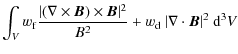
L	=	$\displaystyle \int_{V} w_{\rm f} \frac{\vert( \nabla \times \vec{B}) \times \vec{B}\vert^2}{B^2} + w_{\rm d} ~\vert\nabla \cdot \vec{B}\vert^2 ~ {\rm d}^3V$
		$\displaystyle ~+ \nu \int_{S} (\vec{B} - \vec{B}_{\rm obs})\cdot\vec{W}\cdot(\vec{B} - \vec{B}_{\rm obs}) {\rm d}^2S .$	(4)

The first integral contains the conditions (1) and (2) as quadratic forms and obviously for $w_{\rm f}, w_{\rm d} >0$ that the force-free conditions (1, 2) are fulfilled when the functional reaches its minimum at L=0. This was the approach used in before (see Wiegelmann 2004; Wheatland et al. 2000, for details) where the boundary conditions entered directly as iterative improvements of $\vec{B}$ to minimize L were constrained to $\vec{B}=\vec{B}_{\rm obs}$ at the photospheric boundary.

Here, we propose to extend the functional by adding the surface integral over the photosphere (4) and iterating $\vec{B}$ to minimize L, which is otherwise unconstrained. In this integral, $\vec{W}(x,y)$ is a diagonal error matrix, the elements $w_{\rm los},w_{\rm trans},w_{\rm trans}$ of which are chosen inversely proportional to the local measurement error of the respective photospheric field component at x,y. In principle $\vec{W}$ should be specified by the instrument, and it is likely that this error distribution will be provided along with the data for SDO/HMI vector magnetograms. Because the line-of-sight photospheric magnetic field is measured with much higher accuracy than the transverse field $B_{\rm trans}$ , we typically set the component $w_{\rm los}$ to unity, while the transverse components of $w_{\rm trans}$ are typically small but positive. In regions where $B_{\rm trans}$ has not been measured or where the signal-to-noise ratio is very poor, we set $w_{\rm trans}=0$ .

The boundary value problem (1) and (2) is nonlinear, and there is no guarantee that a solution exists for all sets of boundary values in the sense that we can obtain L=0exactly. Boulmezaoud & Amari (2000) have shown that the full vector field as boundary condition overdetermines the problem, and Wiegelmann et al. (2010) investigated the influence of photospheric measurement errors. Observed and noisy boundary fields $\vec{B}_{\rm obs}$ are very probably inconsistent and belong to the set of boundary values for which a strict solution does not exist. In these cases the first integral in (4) alone could often not be iterated to values of the order of the numerical roundoff-error. With the new formulation (4) we allow deviations between the model field $\vec{B}$ and the observed $\vec{B}_{\rm obs}$ and so the model field can be iterated closer to a force-free field even if the observations are inconsistent. This balance is controlled by the Lagrangian multiplier $\nu$ .

2.1 Encoding of old code

The previous version of our optimisation code worked as follows (see also Wiegelmann 2004, for details):

Set initial $\vec{B}$ to the potential field computed from the normal component of $\vec{B}_{\rm obs}$ at the photospheric boundary.
Replace the transverse field component of the initial $\vec{B}$ by the observed field components of $\vec{B}_{\rm obs}$ at the photospheric boundary.
Minimise L (Eq. (4)) iteratively, keeping $\vec{B}$ unchanged at the photospheric boundary. Only the first two terms are influenced and the surface integral vanishes by construction at each iteration step.

2.2 Encoding of new code

Set initial $\vec{B}$ to the potential field computed from the normal component of $\vec{B}_{\rm obs}$ at the photospheric boundary as above.
Minimise L (Eq. (4)) iteratively without constraining $\vec{B}$ at the photospheric boundary. The transverse magnetic field $B_{\rm trans}$ is gradually driven towards the observations while the field relaxes to a force-free field. If the observed field is inconsistent, the difference $\vec{B} - \vec{B}_{\rm obs}$ remains finite depending on the control parameter $\nu$ . Where $w_{\rm trans}=0$ the observed field is automatically ignored.
Different from the old code the magnetic field is also relaxed in the bottom boundary. Consequently the boundary values of $B_{\rm trans}$ in regions with poor signal to noise ratio ( $w_{\rm trans}=0$ ) are automatically relaxed towards force-free consistent values.
The state L=0 corresponds to a perfect force-free and divergence-free state and exact agreement of the boundary values $B_{\rm trans}$ with observations in regions with $w_{\rm trans}>0$ . For inconsistent boundary data the force-free and solenoidal conditions can still be fulfiled, but the third surface term will remain finite. This results in some deviation of the bottom boundary data from the observations in regions, where $w_{\rm trans}$ is small.

For both codes the iteration stops when L becomes stationary. Numerically stationarity is assumed when $\frac{{\rm d}L }{{\rm d}t}/L < 10^{-4}$ for 100 consecutive iteration steps.

Table 1: Evaluation of the reconstruction quality.

$\begin{figure} \par\includegraphics[width=14cm,clip]{14391f1NEW.eps}\vspace*{-2mm} \end{figure}$	Figure 1: Magnetic fieldline plots for the reference equilibrium (panel a)), the initial potential field b) and the other panels show nonlinear force-free reconstructions with the old and new code for different cases, see text.
Open with DEXTER

$\begin{figure} \par\includegraphics[width=18cm,clip]{14391f2NEW.eps} \end{figure}$	Figure 2: Evolution of the entire functional L (solid line, see Eq. (4)) and its three terms (see Eq. (5)-(7)).
Open with DEXTER

3 Code testing

We tested the new code with the well known semi-analytic equilibrium from Low & Lou (1990). These are force-free axis-symmetric equilibria in spherical geometry, but the symmetry has broken for our tests by cutting a rectangular obliquely orientated box out of the spherical solution. By means of a linear shift l and a rotation angle $\Phi$ , we positioned the centre of the equilibrium solution and tilted its axis orientation relative to the cartesian geometry of the computational domain (see Low & Lou 1990, for details). These equilibria have become a standard for testing nonlinear force-free extrapolation codes, (see, e.g., Tadesse et al. 2009; Wiegelmann & Neukirch 2003; Amari et al. 2006; Inhester & Wiegelmann 2006; Schrijver et al. 2006; Valori et al. 2007; Wheatland et al. 2000, for earlier studies with this equilibrium). We here chose l=0.3 and $\Phi=0.15 \pi$ for our tests and computed the equilibrium in a box with nx=ny=80, nz=72.

Table 1 shows the results of these tests, where Col. 1 names the used code. The second and third column list the values of the new parameters for the code in (4), the Lagrangian multiplier $\nu$ and the matrix element $w_{\rm trans}$ while $w_{\rm los}$ was set to unity throughout.

These parameters were not present in the old code.

We treated the equilibrium field on the bottom boundary as the observed field $\vec{B}_{\rm obs}$ input for both our old and new extrapolation code. After the extrapolation, we evaluated the quality of our reconstruction by comparing the extrapolation result with the exact reference solution in the center 64³ cube by a number of figures of merit in Table 1 Cols. 4-8. These are the vector correlation (VC), Chauchy Schwarz (CS), normalized vector error (NE), mean vector error (ME) and the ratio of the computed magnetic energy and the energy of the Low and Lou reference field (Energy). For a perfect reconstruction NE and ME are zero and all other quantities are unity (see Schrijver et al. 2006, for a detailed explanation of these figures and the corresponding mathematical equations).

We also evaluated how well the force-free condition

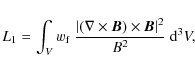
$\begin{displaymath}L_1= \int_{V} w_{\rm f} ~ \frac{\vert( \nabla \times \vec{B}) \times \vec{B}\vert^2}{B^2} ~ {\rm d}^3V, \end{displaymath}$

(5)

the divergence-free condition

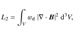
$\begin{displaymath}L_2=\int_{V} w_{\rm d} ~ \vert\nabla \cdot \vec{B}\vert^2 ~ {\rm d}^3V, \end{displaymath}$

(6)

and the boundary data term

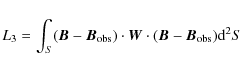
$\begin{displaymath}L_3=\int_{S} (\vec{B} - \vec{B}_{\rm obs})\cdot\vec{W}\cdot(\vec{B} - \vec{B}_{\rm obs}) {\rm d}^2S \end{displaymath}$

(7)

are satisfied. The respective numbers are listed in Table 1 in Cols. 9 and 10. The last column displays the number of iteration steps needed to obtain the reconstruction. In practical computations L₁, L₂ and L₃ never vanish exactly, but the code stops when $\sum_i L_i$ becomes more or less stationary. The final values of L₁, L₂ may be high if the imposed boundary conditions are inconsistent. In this case a force-free solution that matches the boundary fields does not exist. However, even for consistent boundary conditions L₁ and L₂ remain finite for numerical reasons. As a typical error we expect $L \simeq N^3 (10^{-5}/\Delta x)^2$ , where $\Delta x=1/N$ is the grid spacing and N the number of grid points along each axis. For N=64 this yields $L\simeq 0.1$ . The typical discretisation error can be estimated from the entries for the analytical solution in the first row and for the potential field in the second row. They are of the same order of magnitude as the estimated error above except for L₁ of the potential field, which diminishes to roundoff errors because it was obtained from a numerical gradient of a potential. An iterative solution of the potential field gave residual values for both, L₁ and L₂slightly below the estimated numerical error of 0.1.

3.1 Tests with ideally measured boundary conditions

The first two rows in Table 1 show for reference the figures of merit for the original reference solution and the initial potential field, respectively. Rows 3-9 display test results with ideal boundary conditions $\vec{B}_{\rm obs}$ from the exact solution. For the new code we varied the Lagrangian multiplier $\nu$ and the matrix elements $w_{\rm trans}$ . For $w_{\rm trans}=1$ all pixels in the magnetogram are treated equally, which is reasonable for perfectly measured data. Figure 1c and 1d show the respective reconstructed field lines with the old and new code $(w_{\rm trans}=1, \nu=0.01)$ , respectively. Within a reasonable range of parameters the new code gives the same result as the old one. If the Lagrangian multiplier $\nu$ is chosen too small or $w_{\rm trans}$ is nonzero mainly only for strong field regions, the reconstructed solution is gradually decoupled from $\vec{B}_{\rm obs}$ and the resulting field deviates from the exact solution towards a potential field. For $\nu=0$ the code should stop immediately and return the initial potential field for which L₁=L₂=0. For $\nu\rightarrow\infty$ the bottom boundary field is forced to agree with $\vec{B}_{\rm obs}$ at every iteration step and the iteration should perform as for the old code.

A main difference between old and new code is the evolution of the functional L during the iteration as shown in Fig. 2 panel a) and b). For the new code the force-part L₁ and divergence-part L₂ remain small during the entire iteration. The final state is almost identical for both implementations, however.

3.2 Tests with boundary conditions with lacking data

The main reason for the new implementation of our code is that we need to deal with boundary data of different noise levels and qualities or even miss some data points completely. This occurs e.g. due to the limited field of view of some vector magnetographs like Hinode-SOT. The line-of-sight magnetic field is usually available for the entire solar disk, e.g. from SOHO/MDI, but the transverse components $B_{\rm trans}$ are often not available in parts of an active region. SDO/HMI will observe full-disk vector-magnetograms, but $B_{\rm trans}$ will suffer from a poor signal-to-noise ratio in weak field regions. This makes $B_{\rm trans}$ measurements less reliable in these regions.

We mimiced this effect by removing the information regarding the transverse field in certain areas, e.g. where $\vert B_{\rm trans}\vert < 0.05 \max(\vert B_{\rm trans}\vert)$ and $\vert B_{\rm trans}\vert < 0.1 \max(\vert B_{\rm trans}\vert)$ , respectively. For our test field, this affects $73 \%$ and $85 \%$ of the bottom boundary, respectively. Finally as an extreme test we assigned $B_{\rm trans}$ only in a very restricted area close to a local field concentration. This simulates measurements with a vector magnetograph of a very small FOV. For our test field $B_{\rm trans}$ is then available for only $5\%$ of the bottom boundary. In the new code, the boundary area with lacking data is marked by $w_{\rm trans}=0$ , in the old code the lacking transverse field components are filled with zeros, which implies a vertical magnetic field (see DeRosa et al. 2009, for details.)

The fieldline plots from these latter two reconstructions are shown in Fig. 1e-h. The comparison with the exact solution and numerical residuals of the $\vec{j}~\times~\vec{B}$ force and the divergence are displayed in rows 10-18 of Table 1. We find that the new code is closer to a force- and divergence-free field in all cases and L₁ and L₂ are significantly smaller, in particular for low values of the Lagrangian multiplier $\nu$ . The result of the new code agrees also somewhat better with the original solution than the output of the old code, but the difference is not as significant as the difference in force-free and solenoidal conditions.

The reason for these results is that the old and new code react differently to inconsistent boundary conditions caused by noisy data and by assuming a vertical field in regions where transversal field measurements are lacking. As seen in Fig. 2 panel c) the functional L iterated in the old code soon reaches a stationary state at a finite value of L if the boundary data are inconsistent. This is different with the new code, shown in panels d) and e). Here L₁ and L₂ remain very small during the entire evolution and the inconsistency in the boundary data is absorbed in the L₃ term. L₃ can also become relatively low however, because regions with $w_{\rm trans}=0$ (where the transverse field has a poor signal-to-noise ratio or is even unknown) do scarcely or not at all contribute to the functional. For a reasonably small Lagrangian multiplier $\nu$ as shown in panel e) the functionals L₁ and L₂ stay at a very low level (discretisation error). The new code also relaxes the bottom boundary values and changes the field there in order to find force-free consistent boundary conditions. If information on $B_{\rm trans}$ are lacking in a significant part of the magnetogram (up to $95 \%$ of the pixels in our example), there is no unique solution for consistently specifying $B_{\rm trans}$ , and one cannot expect the final equilibrium to agree with the model solution. Yet we have the most probable magnetic field model, because it is close to force- and divergence-free and agrees with the sparse observed boundary data.

3.3 Influence of noise

Finally we investigate how noise influences the quality of the reconstructed magnetic field in the last three rows of Table 1. We added a uniform noise of $5\%$ of the maxim transversal magnetic field onto $B_{\rm trans}$ For the old code the inconsistency in the boundary data leads to significant deviations from the force-free L₁ and solenoidal condition L₂. Computations with the new code lead to significantly better agreement of the force and solenoidal condition, e.g., by almost two orders of magnitude for a small Lagrangian multiplier $\nu=0.001$ . The effect of noise in the transversal field is similar to lacking data, which is natural, as regions with a very poor signal-to-noise ratio in $B_{\rm trans}$ can be as well considered as regions where we do not know $B_{\rm trans}$ . The new code still finds a force-free solution for these cases, which are, however, more potential field like than the solution with full information. But even for this relatively high noise level the reconstructed solution still has similarities to the original Low and Lou reference field (error of $3{-}4 \%$ in the vector correlation and an under-estimation of the energy of $12{-}14 \%$ .) and is a significantly better approximation than a potential field, which as an error of $12 \%$ and $33 \%$ for the vector correlation and energy estimate, respectively.

4 Conclusions

Different from previous implementations our new code allows us to deal with lacking data and regions with poor signal-to-noise ratio in the extrapolation in a systematic manner because it produces a field which is closer to to a force- and divergence-free field and tries to match the boundary only where it has been reliably measured. For ideal and consistent data the extrapolation result is identical with previous implementations of our code. This old result could also artificially be enforced by the choice $\nu\rightarrow\infty$ and $w_{\rm trans}=1$ .

For finite $\nu$ , the new code also relaxes the boundary and allows us to fulfill the solenoidal and force-free condition significantly better because it allows deviations between the extrapolated boundary field and inconsistent boundary data. This deviation can be controlled by setting the weight factors $w_{\rm trans}$ inversely proportional to the measurement error or $w_{\rm trans}=0$ , where the field information is lacking.

If no transverse magnetic field has been observed on a significant part of the vector magnetogram, the magnetic energy of the final relaxed state is underestimated. In an extreme case when no $B_{\rm trans}$ at all is available in the entire region, the code would produce the initial potential field.

Acknowledgements

The work of T. Wiegelmann was supported by DLR-grant 50 OC 0501. This work was inspired by discussions with our colleagues in the NLFFF-consortium (a group of scientist sharing their experience on nonlinear force-free field modelling) during six annual workshops in the years 2004-2009.

References

Amari, T., Boulmezaoud, T. Z., & Aly, J. J. 2006, A&A, 446, 691 [NASA ADS] [CrossRef] [EDP Sciences] [Google Scholar]
Boulmezaoud, T. Z., & Amari, T. 2000, Z. Angew. Math. Phys., 51, 942 [Google Scholar]
DeRosa, M. L., Schrijver, C. J., Barnes, G., et al. 2009, ApJ, 696, 1780 [Google Scholar]
Fuhrmann, M., Seehafer, N., & Valori, G. 2007, A&A, 476, 349 [NASA ADS] [CrossRef] [EDP Sciences] [Google Scholar]
Inhester, B., & Wiegelmann, T. 2006, Sol. Phys., 235, 201 [NASA ADS] [CrossRef] [Google Scholar]
Low, B. C., & Lou, Y. Q. 1990, ApJ, 352, 343 [NASA ADS] [CrossRef] [Google Scholar]
Metcalf, T. R., Derosa, M. L., Schrijver, C. J., et al. 2008, Sol. Phys., 247, 269 [Google Scholar]
Schrijver, C. J., Derosa, M. L., Metcalf, T. R., et al. 2006, Sol. Phys., 235, 161 [Google Scholar]
Tadesse, T., Wiegelmann, T., & Inhester, B. 2009, A&A, 508, 421 [NASA ADS] [CrossRef] [EDP Sciences] [Google Scholar]
Valori, G., Kliem, B., & Fuhrmann, M. 2007, Sol. Phys., 245, 263 [NASA ADS] [CrossRef] [Google Scholar]
Wheatland, M. S., Sturrock, P. A., & Roumeliotis, G. 2000, ApJ, 540, 1150 [Google Scholar]
Wiegelmann, T. 2004, Sol. Phys., 219, 87 [NASA ADS] [CrossRef] [Google Scholar]
Wiegelmann, T., & Neukirch, T. 2003, Nonlin. Processes Geophys., 10, 313 [Google Scholar]
Wiegelmann, T., Inhester, B., & Sakurai, T. 2006, Sol. Phys., 233, 215 [NASA ADS] [CrossRef] [Google Scholar]
Wiegelmann, T., Thalmann, J. K., Schrijver, C. J., Derosa, M. L., & Metcalf, T. R. 2008, Sol. Phys., 247, 249 [NASA ADS] [CrossRef] [Google Scholar]
Wiegelmann, T., Yelles Chaouche, L., Solanki, S. K., & Lagg, A. 2010, A&A, 511, A4 [Google Scholar]

Footnotes

... throughout: We investigated several forms of $w_{\rm trans}$ as indicated in the third column of the table. 1,0 means that we chose $w_{\rm trans}=1$ in the valid $B_{\rm trans}$ area and 0 elsewhere.
...: This would correspond to a noise level of about 100 G for real measurements.

All Tables