| Issue |
A&A
Volume 516, June-July 2010
|
|
|---|---|---|
| Article Number | A18 | |
| Number of page(s) | 8 | |
| Section | Astrophysical processes | |
| DOI | https://doi.org/10.1051/0004-6361/201014023 | |
| Published online | 17 June 2010 | |
Relativistic Doppler-boosted emission in gamma-ray binaries
G. Dubus - B. Cerutti - G. Henri
Laboratoire d'Astrophysique de Grenoble, UMR 5571 Université Joseph Fourier Grenoble I/CNRS, BP 53, 38041 Grenoble, France
Received 8 January 2010 / Accepted 29 March 2010
Abstract
Context. Gamma-ray binaries could be compact pulsar wind
nebulae formed when a young pulsar orbits a massive star. The pulsar
wind is contained by the stellar wind of the O or Be companion,
creating a relativistic comet-like structure accompanying the pulsar
along its orbit.
Aims. The X-ray and the very high energy (>100 GeV, VHE)
gamma-ray emission from the binary LS 5039 are modulated on the orbital
period of the system. Maximum and minimum flux occur at the
conjunctions of the orbit, suggesting that the explanation is linked to
the orbital geometry. The VHE modulation has been proposed to be due to
the combined effect of Compton scattering and pair production on
stellar photons, both of which depend on orbital phase. The X-ray
modulation could be due to relativistic Doppler boosting in the comet
tail where both the X-ray and VHE photons would be emitted.
Methods. Relativistic aberrations change the seed stellar photon
flux in the comoving frame so Doppler boosting affects synchrotron and
inverse Compton emission differently. The dependence with orbital phase
of relativistic Doppler-boosted (isotropic) synchrotron and
(anisotropic) inverse Compton emission is calculated, assuming that the
flow is oriented radially away from the star (LS 5039) or
tangentially to the orbit (LS I +61
![]() 303, PSR B1259-63).
303, PSR B1259-63).
Results. Doppler boosting of the synchrotron emission in
LS 5039 produces a lightcurve whose shape corresponds to the X-ray
modulation. The observations imply an outflow velocity of 0.15-0.33c consistent with the expected flow speed at the pulsar wind termination shock. In LS I +61
![]() 303, the calculated Doppler boosted emission peaks in phase with the observed VHE and X-ray maximum.
303, the calculated Doppler boosted emission peaks in phase with the observed VHE and X-ray maximum.
Conclusions. Doppler boosting is not negligible in gamma-ray
binaries, even for mildly relativistic speeds. The boosted modulation
reproduces the X-ray modulation in LS 5039 and could also provide
an explanation for the puzzling phasing of the VHE peak in
LS I +61
![]() 303.
303.
Key words: radiation mechanisms: non-thermal - gamma rays: stars - X-rays: binaries - astroparticle physics
1 Introduction
Gamma-ray binaries display non-thermal emission from radio to very
high energy gamma rays (VHE, >100 GeV). Their spectral
luminosities peak at energies greater than a MeV. At present,
three such systems are known: PSR B1259-63 (Aharonian et al. 2005b), LS 5039 (Aharonian et al. 2005a) and LS I +61
![]() 303 (Albert et al. 2006). A fourth system, HESS J0632+057 may also be a gamma-ray binary (Hinton et al. 2009).
The systems are composed of a O or Be massive star and a compact
object, identified as a young radio pulsar in PSR B1259-63. All
gamma-ray binaries could harbour young pulsars (Dubus 2006).
303 (Albert et al. 2006). A fourth system, HESS J0632+057 may also be a gamma-ray binary (Hinton et al. 2009).
The systems are composed of a O or Be massive star and a compact
object, identified as a young radio pulsar in PSR B1259-63. All
gamma-ray binaries could harbour young pulsars (Dubus 2006).
Electrons accelerated in the binary system upscatter UV photons from the companion to gamma-ray energies. The Compton scattered radiation received by the observer is anisotropic because the source of seed photons is the companion star. VHE gamma-rays will also produce e+e- pairs as they propagate through the dense radiation field, absorbing part of the primary emission. This is also anisotropic. Both effects combine to produce an orbital modulation of the gamma-ray flux if the electrons are in a compact enough region. This modulation depends only on the geometry. Orbital modulations of the high-energy (HE, >100 MeV) and VHE fluxes have indeed been observed. The modulations unambiguously identify the gamma-ray source with the binary (Albert et al. 2006; Acciari et al. 2008; Aharonian et al. 2006).
Synchrotron emission can dominate over inverse Compton scattering at X-ray energies, providing additional information to disentangle geometrical effects from intrinsic variations of the source. Suzaku and INTEGRAL observations of LS 5039 have revealed a stable modulation of the X-ray flux (Hoffmann et al. 2009; Takahashi et al. 2009). Possible interpretations are discussed in Sect. 2. None are satisfying. The key point is that the X-ray flux is maximum and minimum at conjunctions and that this excludes any explanation unrelated to the system's geometry as seen by the observer.
In the pulsar wind scenario, the synchrotron emission is expected to
arise in shocked pulsar wind material collimated by the stellar wind.
This creates a cometary tail with a mildly relativistic bulk motion
(Fig. 1).
Relativistic Doppler boosting of the emission due to this bulk motion
is calculated in Sect. 3 with details given in Appendix A. The
orbital motion leads to a modulation of the Doppler boost, as
previously proposed in the context of black widow pulsars (Huang & Becker 2007; Arons & Tavani 1993).
The calculated synchrotron modulation is similar to that seen in X-rays
in LS 5039. Although this is not formally confirmed due to their
long orbital periods, LS I +61
![]() 303 and PSR B1259-63 also appear to have modulated X-ray emission (Chernyakova et al. 2006,2009; Acciari et al. 2009; Anderhub et al. 2009). The application to these gamma-ray binaries is discussed in Sect. 4.
303 and PSR B1259-63 also appear to have modulated X-ray emission (Chernyakova et al. 2006,2009; Acciari et al. 2009; Anderhub et al. 2009). The application to these gamma-ray binaries is discussed in Sect. 4.
![\begin{figure}
\par\includegraphics[width=7cm,clip]{14023fig1}
\end{figure}](/articles/aa/full_html/2010/08/aa14023-10/img14.png)
|
Figure 1: Geometry of Doppler
boosted emission from a collimated shock pulsar wind nebula. The orbit
is that of LS 5039 (to scale). The comet tail moves away from the
pulsar with a speed |
| Open with DEXTER | |
2 The X-ray modulation in LS 5039
2.1 X-ray observations
LS 5039 has shown steady, hard X-ray emission since its discovery (Martocchia et al. 2005; Ribó et al. 1999; Motch et al. 1997; Reig et al. 2003; Bosch-Ramon et al. 2005,2007). RXTE observations hinted at orbital variability (Bosch-Ramon et al. 2005) but confirmation had to wait the Suzaku and INTEGRAL observations (Hoffmann et al. 2009; Takahashi et al. 2009). The average spectrum seen by Suzaku from 0.6 keV to 70 keV is an absorbed power-law with spectral index
![]() (
(
![]() )
and
)
and
![]() cm-2 and
cm-2 and
![]() erg cm-2 s-1, consistent with previous observations. There is no evidence for a cutoff up to 70 keV.
erg cm-2 s-1, consistent with previous observations. There is no evidence for a cutoff up to 70 keV.
Variability in Suzaku is dominated by a well-resolved
modulation followed over an orbit and a half. The X-ray flux varies by
a factor 2 with a minimum at
![]() ,
slightly after superior conjunction (
,
slightly after superior conjunction (
![]() based on Aragona et al. 2009) and a maximum at inferior conjunction (
based on Aragona et al. 2009) and a maximum at inferior conjunction (
![]() ). The 1-10 keV photon index is also modulated, varying between 1.61
). The 1-10 keV photon index is also modulated, varying between 1.61![]() at minimum flux and
at minimum flux and
![]() at maximum flux. The comparison with Chandra and XMM measurements suggests the modulation is stable on timescales of years (Kishishita et al. 2009).
The column density is constant with orbital phase, as if there were
only absorption from the ISM. The lack of significant wind absorption
suggests that the X-ray source is located far from the system or that
the wind is highly ionised and/or has a mass-loss rate
at maximum flux. The comparison with Chandra and XMM measurements suggests the modulation is stable on timescales of years (Kishishita et al. 2009).
The column density is constant with orbital phase, as if there were
only absorption from the ISM. The lack of significant wind absorption
suggests that the X-ray source is located far from the system or that
the wind is highly ionised and/or has a mass-loss rate ![]()
![]() (Bosch-Ramon et al. 2007). Here, we assume that the X-ray source is situated within the orbital system.
(Bosch-Ramon et al. 2007). Here, we assume that the X-ray source is situated within the orbital system.
2.2 Inverse Compton X-ray emission?
The phases of X-ray and VHE maximum (minimum) are identical. If both
are due to inverse Compton scattering off stellar photons then maximum
emissivity is at superior conjunction. Subsequent in-system absorption
due to pair production moves the observed VHE maximum flux to the
inferior conjunction. X-ray photons are too weak for pair production
but could be absorbed in the stellar wind with a similar result. This
can be ruled out since the modulation is seen in hard X-rays above
10 keV and ![]() is constant with orbital phase. Thomson scattering of the hard X-rays
is unlikely as it would require a column density of scattering
electrons
is constant with orbital phase. Thomson scattering of the hard X-rays
is unlikely as it would require a column density of scattering
electrons ![]() 1024 cm-2
(e.g. a Wolf-Rayet wind as in Cyg X-3 rather than an O star wind), two
orders-of-magnitude above the observed absorbing column density and
plausible stellar wind column densities.
1024 cm-2
(e.g. a Wolf-Rayet wind as in Cyg X-3 rather than an O star wind), two
orders-of-magnitude above the observed absorbing column density and
plausible stellar wind column densities.
2.3 Synchrotron X-ray emission?
Alternatively, the X-ray emission is synchrotron radiation from the same electrons that emit HE and VHE ![]() -rays. In Dubus et al. (2008), we proposed that several features of the VHE observations could be explained by assuming continuous injection of a E-2 power-law of electrons at the location of the compact object in a zone with a homogeneous magnetic field B of order 1 G (Dubus et al. 2008).
The synchrotron X-ray spectrum expected in this model
-rays. In Dubus et al. (2008), we proposed that several features of the VHE observations could be explained by assuming continuous injection of a E-2 power-law of electrons at the location of the compact object in a zone with a homogeneous magnetic field B of order 1 G (Dubus et al. 2008).
The synchrotron X-ray spectrum expected in this model![]() is shown in Fig. 2. It is hard with
is shown in Fig. 2. It is hard with
![]() .
The electrons producing this X-ray synchrotron emission have energies
between 10 GeV and 1 TeV, for which the dominant cooling
mechanism is inverse Compton scattering in the Klein-Nishina regime.
This keeps the steady-state distribution close to the E-2 power law (Fig. 3 in Dubus et al. 2008). Synchrotron cooling takes over at higher energies, causing a break to
.
The electrons producing this X-ray synchrotron emission have energies
between 10 GeV and 1 TeV, for which the dominant cooling
mechanism is inverse Compton scattering in the Klein-Nishina regime.
This keeps the steady-state distribution close to the E-2 power law (Fig. 3 in Dubus et al. 2008). Synchrotron cooling takes over at higher energies, causing a break to
![]() .
In fact, the spectral index seen by INTEGRAL up to 200 keV is softer (
.
In fact, the spectral index seen by INTEGRAL up to 200 keV is softer (
![]() )
than the average index measured by Suzaku up to 70 keV (
)
than the average index measured by Suzaku up to 70 keV (
![]() ).
).
Whereas it is promising to have the hard X-ray spectral shape correctly reproduced, the level of X-ray emission is too low and, more importantly, the orbital X-ray lightcurve from the model is inconsistent with the observed modulation. The expected 1-10 keV lightcurve shows only a very modest change with a peak at periastron (Fig. 2). The reason is that the variations in particle and magnetic energy densities (a factor 4) compensate to keep the synchrotron emission almost constant.
![\begin{figure}
\par\includegraphics[width=8.8cm,clip]{14023fig2a}\vspace*{2.8mm}
\hspace*{2.8mm}\includegraphics[width=8.5cm,clip]{14023fig2b}
\end{figure}](/articles/aa/full_html/2010/08/aa14023-10/img32.png)
|
Figure 2: Comparison of the model for LS 5039 described in Sect. 2.3 with observations. Top panel: spectral energy distribution showing the Suzaku 1-10 keV maximum and minimum spectra (Takahashi et al. 2009), the 100 MeV-10 GeV average Fermi spectrum (Abdo et al. 2009b) and the VHE spectra averaged over phases INFC (dark points) and SUPC (grey points) as defined in Aharonian et al. (2006). The model spectra averaged over INFC and SUPC are shown as dark and grey curves. Middle and bottom panels: expected VHE gamma-ray and X-ray orbital modulation compared to the HESS and Suzaku observations. |
| Open with DEXTER | |
2.4 Variations in parameters?
A better fit is possible by treating B or particle injection as free functions of orbital phase or by taking adiabatic losses into account. Takahashi et al. (2009) argued that the X-ray spectrum necessarily implies dominant adiabatic cooling of an E-2
electron distribution (this is sufficient but not necessary: as
discussed above, Klein-Nishina cooling also keeps the distribution
hard). The X-ray and VHE observations were then be fitted by adjusting
the adiabatic timescale
![]() with orbital phase. The derived variation in
with orbital phase. The derived variation in
![]() mirrors the X-ray lightcurve with
mirrors the X-ray lightcurve with
![]() reaching a maximum at
reaching a maximum at
![]() .
There is no obvious reason why
.
There is no obvious reason why
![]() should peak at this phase. Takahashi et al. (2009) expect the variation in
should peak at this phase. Takahashi et al. (2009) expect the variation in
![]() to reflect variations in the size of the emitting zone, itself
modulated by the external pressure of the wind. The relevant phases are
those of apastron (low pressure) and periastron (high pressure), but
not inferior conjunction which is an observer-dependent phase unrelated
to wind pressure. In LS 5039,
to reflect variations in the size of the emitting zone, itself
modulated by the external pressure of the wind. The relevant phases are
those of apastron (low pressure) and periastron (high pressure), but
not inferior conjunction which is an observer-dependent phase unrelated
to wind pressure. In LS 5039,
![]() is significantly different from the phases of periastron and apastron
passage. Hence, it would require a coincidence for any intrinsic change
in the source (B, number of particles,
is significantly different from the phases of periastron and apastron
passage. Hence, it would require a coincidence for any intrinsic change
in the source (B, number of particles,
![]() ,
size, etc.) to result in a peak at this conjunction.
,
size, etc.) to result in a peak at this conjunction.
The link between the extrema of the X-ray lightcurve and conjunctions calls for a geometrical explanation related to how the observer views the X-ray source. Doppler boosting (see Fig. 1) is a possible solution to this puzzle.
3 Relativistic Doppler boosting
In the interacting winds scenario, the X-ray emission is expected to occur beyond the shock where the ram pressures balance (Dubus 2006; Maraschi & Treves 1981; Tavani et al. 1994; Bignami et al. 1977).
Particles in the shocked pulsar wind are randomized and accelerated.
MHD jump conditions for a perpendicular shock and a low magnetisation
pulsar wind give a post-shock flow speed of c/3 (Kennel & Coroniti 1984). If the ratio of wind momenta
![]() is small then the shocked pulsar wind is confined by the stellar wind.
The shocked wind flows away from the companion star forming a
comet-like tail of emission. Relativistic hydrodynamical calculations
show the flow is conical with an opening angle set by
is small then the shocked pulsar wind is confined by the stellar wind.
The shocked wind flows away from the companion star forming a
comet-like tail of emission. Relativistic hydrodynamical calculations
show the flow is conical with an opening angle set by ![]() and can reach highly relativistic speeds (Bogovalov et al. 2008).
High energy electrons emit VHE gamma-rays and synchrotron X-rays close
to the pulsar and lose energy as they flow out, emitting in the radio
band far from the system (Dubus 2006). Here, the relativistic electrons radiating X-rays (by synchrotron) and VHE
and can reach highly relativistic speeds (Bogovalov et al. 2008).
High energy electrons emit VHE gamma-rays and synchrotron X-rays close
to the pulsar and lose energy as they flow out, emitting in the radio
band far from the system (Dubus 2006). Here, the relativistic electrons radiating X-rays (by synchrotron) and VHE ![]() -rays
(by inverse Compton) are assumed to be localized at the compact object
location. The calculation of the relativistic Doppler boosting in the
flow is general and can also be applied e.g. to the case of a
relativistic jet in a binary (Dubus et al. 2010).
-rays
(by inverse Compton) are assumed to be localized at the compact object
location. The calculation of the relativistic Doppler boosting in the
flow is general and can also be applied e.g. to the case of a
relativistic jet in a binary (Dubus et al. 2010).
3.1 Synchrotron
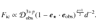
Even if the flow is only mildly relativistic, Doppler boosting can
introduce a geometry-dependent modulation of emission that is isotropic
in the comoving frame (Fig. 1). This will be the case for synchrotron emission. The relativistic boost is given by
where
The outgoing energy will be modified by
![]() and the outgoing flux will be
and the outgoing flux will be
![]() ,
with primed quantities referring to the comoving frame.
In the case of a constant synchrotron power-law spectrum in the comoving frame with index
,
with primed quantities referring to the comoving frame.
In the case of a constant synchrotron power-law spectrum in the comoving frame with index ![]() then
then

The ratio of maximum to minimum flux is (see also Pelling et al. 1987)
for
3.2 Inverse Compton
Inverse Compton emission will also be modified by relativistic
aberration. The spectrum of the target photons seen in a given solid
angle in the comoving flow frame will be changed according to a
different relativistic transform. If the star is assumed to be
point-like, the relativistic boost involved is
|
(4) |
The total energy density from the star in the flow frame is
|
(5) |
with the Stefan-Boltzmann constant
Because of this double transform, and because of the intrinsic
orbital phase dependence of scattering on stellar photons, the
Doppler-boosted inverse Compton flux variability can be quite different
from the Doppler-boosted synchrotron variability. In the case of
Thomson scattering off a power-law of electrons d
![]() d
d![]() (see Appendix A)
(see Appendix A)
Note that
![\begin{figure}
\par\includegraphics[width=9cm,clip]{14023fig3}
\end{figure}](/articles/aa/full_html/2010/08/aa14023-10/img54.png)
|
Figure 3:
Doppler-boosted synchrotron (
|
| Open with DEXTER | |
4 Discussion
The Doppler-boosted synchrotron (
![]() ,
Eq. (2)) and inverse Compton (
,
Eq. (2)) and inverse Compton (
![]() ,
Eq. (6))
intensity variations were calculated for the three gamma-ray binaries
and are discussed here. Full calculations were also carried out for
LS 5039 and LS I +61
,
Eq. (6))
intensity variations were calculated for the three gamma-ray binaries
and are discussed here. Full calculations were also carried out for
LS 5039 and LS I +61
![]() 303. The orbital parameters are taken from Manchester et al. (1995) for PSR B1259-63 and from Aragona et al. (2009) for LS 5039 and LS I +61
303. The orbital parameters are taken from Manchester et al. (1995) for PSR B1259-63 and from Aragona et al. (2009) for LS 5039 and LS I +61
![]() 303. The inclination i is assumed to be
303. The inclination i is assumed to be
![]() for PSR B1259-63, and 60
for PSR B1259-63, and 60
![]() for both LS 5039 and LS I +61
for both LS 5039 and LS I +61
![]() 303 (Dubus 2006).
303 (Dubus 2006).
4.1 LS 5039
LS 5039 has a stellar wind velocity (
![]() km s-1) significantly greater than the compact object orbital velocity (
km s-1) significantly greater than the compact object orbital velocity (
![]() km s-1) so that the cometary flow is assumed to be purely radial (
km s-1) so that the cometary flow is assumed to be purely radial (
![]() ). Doppler boosting leads to peaks and troughs for the synchrotron emission
). Doppler boosting leads to peaks and troughs for the synchrotron emission
![]() at conjunctions as outlined in Sect. 3 (Fig. 3). The amplitude of the inverse Compton flux (
at conjunctions as outlined in Sect. 3 (Fig. 3). The amplitude of the inverse Compton flux (
![]() )
is reduced as the increased scattering rate at superior conjunction is compensated by a deboost of
)
is reduced as the increased scattering rate at superior conjunction is compensated by a deboost of
![]() (and vice-versa at inferior conjunction). The shape of the modulation does not change much. The bottom panel shows that
(and vice-versa at inferior conjunction). The shape of the modulation does not change much. The bottom panel shows that
![]() follows well the Suzaku data when
follows well the Suzaku data when ![]() is adjusted to 0.15 in order to match the X-ray modulation amplitude. The spectral index is fixed to the value observed by Suzaku,
is adjusted to 0.15 in order to match the X-ray modulation amplitude. The spectral index is fixed to the value observed by Suzaku,
![]() (equivalent to p=2
for the electron distribution). However, this assumes the intrinsic
synchrotron emission is constant with orbital phase, unlike what
happens in the model discussed in Sect. 2 and shown in Fig. 2.
(equivalent to p=2
for the electron distribution). However, this assumes the intrinsic
synchrotron emission is constant with orbital phase, unlike what
happens in the model discussed in Sect. 2 and shown in Fig. 2.
The precise relativistic corrections were applied to the model discussed in Sect. 2 (Fig. 2), assuming ![]() .
No other changes were made. The average level of X-ray emission is not
changed much. However, the relativistic corrections move the peak X-ray
flux to superior conjunction and increase the amplitude of the
variations, bringing the model X-ray lightcurve very close to the
observations (shown in the bottom panel of Fig. 2). The spectral shape is slightly harder than the observed one by about 0.15 in the index
.
No other changes were made. The average level of X-ray emission is not
changed much. However, the relativistic corrections move the peak X-ray
flux to superior conjunction and increase the amplitude of the
variations, bringing the model X-ray lightcurve very close to the
observations (shown in the bottom panel of Fig. 2). The spectral shape is slightly harder than the observed one by about 0.15 in the index ![]() .
The orbital modulation of
.
The orbital modulation of ![]() follows the X-ray lightcurve with a hardening of
follows the X-ray lightcurve with a hardening of ![]() from 0.42 (superior conjunction) to 0.30 (inferior conjunction), which is similar in amplitude to the hardening observed by Suzaku
(Sect. 2.1). However, the average level of X-ray emission is
systematically too low compared to the observations. Increasing the
magnetic field by a factor 3 would be sufficient to raise the
level of X-ray flux but this would also modify the VHE spectrum,
bringing the break at a few TeV to energies that are too low. The model
assumes all the emission arises within a single zone and this could
explain this shortcoming. The X-ray (and GeV) emission come from
electrons that have significantly cooled since their injection and,
thus, this emission would be more likely to be affected by a more
detailed model where particle cooling is followed along the flow, as
done in Dubus (2006) based on the Kennel & Coroniti (1984)
model for pulsar wind nebula. Numerical simulations are needed to
provide detailed constraints on the geometry and physical conditions in
the post-shock flow.
from 0.42 (superior conjunction) to 0.30 (inferior conjunction), which is similar in amplitude to the hardening observed by Suzaku
(Sect. 2.1). However, the average level of X-ray emission is
systematically too low compared to the observations. Increasing the
magnetic field by a factor 3 would be sufficient to raise the
level of X-ray flux but this would also modify the VHE spectrum,
bringing the break at a few TeV to energies that are too low. The model
assumes all the emission arises within a single zone and this could
explain this shortcoming. The X-ray (and GeV) emission come from
electrons that have significantly cooled since their injection and,
thus, this emission would be more likely to be affected by a more
detailed model where particle cooling is followed along the flow, as
done in Dubus (2006) based on the Kennel & Coroniti (1984)
model for pulsar wind nebula. Numerical simulations are needed to
provide detailed constraints on the geometry and physical conditions in
the post-shock flow.
As expected, the VHE gamma-ray lightcurve is not affected much
by the corrections because most of the escaping VHE gamma-rays are
emitted close to inferior conjunction (as a result of the
![]() opacity). The modified VHE spectrum for SUPC phases is actually better
than the original model that overestimated the VHE flux at a few TeV.
Pair cascading can fill in the flux between 30 GeV and a few TeV
at this phase (Cerutti et al., submitted). At HE gamma-ray energies, in
the Fermi
range, the average flux level is reduced significantly because most of
the HE gamma rays arise at superior conjunction where the flow deboosts
the emission. Fermi observations of LS 5039 and LS I +61
opacity). The modified VHE spectrum for SUPC phases is actually better
than the original model that overestimated the VHE flux at a few TeV.
Pair cascading can fill in the flux between 30 GeV and a few TeV
at this phase (Cerutti et al., submitted). At HE gamma-ray energies, in
the Fermi
range, the average flux level is reduced significantly because most of
the HE gamma rays arise at superior conjunction where the flow deboosts
the emission. Fermi observations of LS 5039 and LS I +61
![]() 303 show that the HE gamma-ray emission cuts off exponentially at a few GeV, suggesting the emission in the Fermi range (100 MeV-10 GeV) is a distinct component from the shocked flow (Abdo et al. 2009b,a).
This could be due to pulsar magnetospheric emission, in which case the
relativistic corrections and model discussed here will not apply to
the GeV component.
303 show that the HE gamma-ray emission cuts off exponentially at a few GeV, suggesting the emission in the Fermi range (100 MeV-10 GeV) is a distinct component from the shocked flow (Abdo et al. 2009b,a).
This could be due to pulsar magnetospheric emission, in which case the
relativistic corrections and model discussed here will not apply to
the GeV component.
4.2 LS I +61
 303
303
The impact of the relativistic Doppler corrections in LS I +61
![]() 303
(and PSR B1259-63) is more difficult to assess because the
orientation of the cometary flow is uncertain. The wind of the Be
stellar companion is thought to be composed of a fast, tenuous polar
wind and, more prominently, a slow, dense equatorial wind. These
equatorial winds are effectively Keplerian discs with a small outflow
velocity (compared to their angular velocity). If the compact object
moves through this disc, then (neglecting corrections due to the
orbital eccentricity) it is essentially moving through a static medium
in the corotating frame, suggesting the outcome is more likely to be
cometary flow trailing the orbit rather than directed radially away
from the companion star. This will have to be confirmed by numerical
simulations of the interaction.
303
(and PSR B1259-63) is more difficult to assess because the
orientation of the cometary flow is uncertain. The wind of the Be
stellar companion is thought to be composed of a fast, tenuous polar
wind and, more prominently, a slow, dense equatorial wind. These
equatorial winds are effectively Keplerian discs with a small outflow
velocity (compared to their angular velocity). If the compact object
moves through this disc, then (neglecting corrections due to the
orbital eccentricity) it is essentially moving through a static medium
in the corotating frame, suggesting the outcome is more likely to be
cometary flow trailing the orbit rather than directed radially away
from the companion star. This will have to be confirmed by numerical
simulations of the interaction.
VHE observations by the MAGIC and VERITAS collaborations consistently find that the peak VHE emission occurs at phases 0.6-0.7 using the historical radio ephemeris (Acciari et al. 2008; Albert et al. 2009). The best estimation of the periastron passage phase in this ephemeris is 0.275 (Aragona et al. 2009), hence there is an offset of 0.275 between the radio ephemeris used by observers and the one used here. As outlined in Sect. 2, the phases of periastron/apastron passage or the conjunctions are the natural phases where the physical conditions or the configuration of the system would be expected to produce minima or maxima in the lightcurves. The peak VHE flux occurs 2 to 5 days before apastron and is clearly not associated with any of those phases, making it difficult to interpret only with anisotropic inverse Compton emission and pair production.
![\begin{figure}
\par\includegraphics[width=9cm,clip]{14023fig4a}\vspace*{2mm}
\includegraphics[width=9cm,clip]{14023fig4b}
\end{figure}](/articles/aa/full_html/2010/08/aa14023-10/img61.png)
|
Figure 4:
Same as Fig. 1
but with the corrections due to relativistic motion taken into account.
The flow is assumed to originate at the compact object location with |
| Open with DEXTER | |
![\begin{figure}
\par\includegraphics[width=9cm,clip]{14023fig5}
\end{figure}](/articles/aa/full_html/2010/08/aa14023-10/img62.png)
|
Figure 5:
Doppler-boosted synchrotron (
|
| Open with DEXTER | |
Superior conjunction in LS I +61
![]() 303
occurs slightly before periastron passage, and inferior conjunction
slightly after. The inverse Compton peak and trough match exactly with
the conjunctions when there is no correction (top panel, Fig. 5). Doppler corrections have a strong impact on the inverse Compton lightcurve. Figure 5 shows the correction factors for LS I +61
303
occurs slightly before periastron passage, and inferior conjunction
slightly after. The inverse Compton peak and trough match exactly with
the conjunctions when there is no correction (top panel, Fig. 5). Doppler corrections have a strong impact on the inverse Compton lightcurve. Figure 5 shows the correction factors for LS I +61
![]() 303
if the flow velocity vector is taken to be exactly tangent to the
orbit. The maximum boost is around phases 0.3-0.4 and the emission is
deboosted around periastron passage. The effect is strong enough to
push the maximum of
303
if the flow velocity vector is taken to be exactly tangent to the
orbit. The maximum boost is around phases 0.3-0.4 and the emission is
deboosted around periastron passage. The effect is strong enough to
push the maximum of
![]() and
and
![]() at phases 0.57-0.67, using the radio ephemeris, as observed. The
correlated behaviour is also consistent with the X-ray and VHE
observations reported in Anderhub et al. (2009). These conclusions also hold when doing a full calculation (bottom panel, Fig. 5)
to properly take into account the Klein-Nishina cross-section. The
calculation assumed a constant power-law distribution of electrons with
p=2. The VHE spectrum is
at phases 0.57-0.67, using the radio ephemeris, as observed. The
correlated behaviour is also consistent with the X-ray and VHE
observations reported in Anderhub et al. (2009). These conclusions also hold when doing a full calculation (bottom panel, Fig. 5)
to properly take into account the Klein-Nishina cross-section. The
calculation assumed a constant power-law distribution of electrons with
p=2. The VHE spectrum is
![]() because of Klein-Nishina effects and the X-ray spectrum is
because of Klein-Nishina effects and the X-ray spectrum is
![]() ,
both of which agree with observations.
,
both of which agree with observations.
4.3 PSR B1259-63
The case of PSR B1259-63 was also explored under the same assumption as LS I +61
![]() 303 (Fig. 6). The inclination is relatively low
303 (Fig. 6). The inclination is relatively low
![]() so that
so that
![]() is almost symmetric without Doppler corrections (top panel). Looking at
the top two panels, it can be seen that the Doppler corrections have
little impact on the overall lightcurve because of the low inclination.
The bottom panel shows that high Doppler factors can strongly deboost
the overall lightcurve even though the morphology remains roughly the
same. There is no obvious relationship between these curves and the
(sparse) X-ray or VHE observations. Other variability factors probably
dominate in this much wider binary system.
is almost symmetric without Doppler corrections (top panel). Looking at
the top two panels, it can be seen that the Doppler corrections have
little impact on the overall lightcurve because of the low inclination.
The bottom panel shows that high Doppler factors can strongly deboost
the overall lightcurve even though the morphology remains roughly the
same. There is no obvious relationship between these curves and the
(sparse) X-ray or VHE observations. Other variability factors probably
dominate in this much wider binary system.
Bogovalov et al. (2008) carried
out relativistic hydrodynamical simulations of a pulsar wind
interacting with a stellar wind with the specific case of
PSR B1259-63 in mind. They found that the shocked pulsar wind can
accelerate from bulk Lorentz factors ![]() 1
close to the termination shock up to 100 far away. Emission from such
highly relativistic flows is not compatible with observations: the
emission would be strongly deboosted (bottom panel, Fig. 6)
except where (and if) the line-of-sight crosses the relativistic
beaming angle where it would produce a flare. The observed X-ray and
VHE modulations in gamma-ray binaries suggest modest boosting. The
X-ray and VHE emission is more likely to originate close to the
termination shock where the jump conditions for an unmagnetized
relativistic flow give
1
close to the termination shock up to 100 far away. Emission from such
highly relativistic flows is not compatible with observations: the
emission would be strongly deboosted (bottom panel, Fig. 6)
except where (and if) the line-of-sight crosses the relativistic
beaming angle where it would produce a flare. The observed X-ray and
VHE modulations in gamma-ray binaries suggest modest boosting. The
X-ray and VHE emission is more likely to originate close to the
termination shock where the jump conditions for an unmagnetized
relativistic flow give ![]() (Kennel & Coroniti 1984).
(Kennel & Coroniti 1984).
![\begin{figure}
\par\includegraphics[width=9cm,clip]{14023fig6}
\end{figure}](/articles/aa/full_html/2010/08/aa14023-10/img65.png)
|
Figure 6:
Doppler-boosted synchrotron (
|
| Open with DEXTER | |
5 Conclusion
The X-ray orbital modulation of LS 5039 peaks and falls at
conjunctions, suggesting that the underlying mechanism is related to
the geometry seen by the observer. Phase-dependent Doppler boosting of
emission from a mildly relativistic flow provides a viable explanation.
The underlying assumption is that the flow direction changes with
orbital phase, so that even constant intrinsic emission becomes
variable as seen by the observer. The peaks and troughs are at
conjunctions for a flow directed radially away from the star, as
expected if the emission arises from a shocked pulsar wind confined by
the fast stellar wind of its companion (Dubus 2006). A moderate relativistic speed of
![]() or 1/3 is enough to reproduce the morphology of the observed X-ray
lightcurve assuming (resp.) either constant intrinsic emission or the
model of Dubus et al. (2008). Note that these values of
or 1/3 is enough to reproduce the morphology of the observed X-ray
lightcurve assuming (resp.) either constant intrinsic emission or the
model of Dubus et al. (2008). Note that these values of ![]() allow for quite large values of the opening angles. More detailed
calculations assuming a conical geometry for the flow confirmed that
the results were unchanged as long as the angular size of the flow is
smaller than
allow for quite large values of the opening angles. More detailed
calculations assuming a conical geometry for the flow confirmed that
the results were unchanged as long as the angular size of the flow is
smaller than ![]() (if larger, the modulation is dampened). Reproducing the level of X-ray
emission is difficult with a one-zone model as it requires values of
the magnetic field that are a factor 3 above current values, leading to
cutoff in the VHE specta at energies that are too low. A more complex
multi-zone model of the post-shock flow might resolve this discrepancy.
(if larger, the modulation is dampened). Reproducing the level of X-ray
emission is difficult with a one-zone model as it requires values of
the magnetic field that are a factor 3 above current values, leading to
cutoff in the VHE specta at energies that are too low. A more complex
multi-zone model of the post-shock flow might resolve this discrepancy.
Inverse Compton scattering in the flow of external stellar
photons will be modulated differently than intrinsic emission from the
flow. In the case of a radial outflow, the external seed photon flux
will be deboosted at all phases. However, a flow tangent to an
eccentric orbit, as might arise in LS I +61
![]() 303
and PSR B1259-63, can lead both to boosts and deboosts in the
comoving frame depending on orbital phase and thus give rise to complex
modulations. The calculated Doppler corrected emission in
LS I +61
303
and PSR B1259-63, can lead both to boosts and deboosts in the
comoving frame depending on orbital phase and thus give rise to complex
modulations. The calculated Doppler corrected emission in
LS I +61
![]() 303
peaks in phase with the observed VHE maximum. This is noteworthy since
a simple explanation had not yet been proposed for the phase of VHE
(and X-ray) maximum in LS I +61
303
peaks in phase with the observed VHE maximum. This is noteworthy since
a simple explanation had not yet been proposed for the phase of VHE
(and X-ray) maximum in LS I +61
![]() 303.
This explanation requires that the shocked pulsar wind flows along the
orbit, which appears compatible with the radio VLBI images on larger
scales shown in Dhawan et al. (2006).
303.
This explanation requires that the shocked pulsar wind flows along the
orbit, which appears compatible with the radio VLBI images on larger
scales shown in Dhawan et al. (2006).
The present work assumed a pulsar relativistic wind in the orbital
plane but microquasar models have also been proposed for both
LS 5039 and LS I +61
![]() 303.
In this case, the emission arises from a relativistic jet. The jet
angle to the observer remains constant along the orbit and so do
303.
In this case, the emission arises from a relativistic jet. The jet
angle to the observer remains constant along the orbit and so do
![]() and
and
![]() .
Hence, no orbital modulation of intrinsic (synchrotron) X-ray emission
due to Doppler boosting would be expected, apart from the possible
impact of jet precession on timescales longer than the orbital period (Kaufman Bernadó et al. 2002). Doppler boosting in a relativistic jet cannot explain the X-ray modulation in LS 5039 or LS I +61
.
Hence, no orbital modulation of intrinsic (synchrotron) X-ray emission
due to Doppler boosting would be expected, apart from the possible
impact of jet precession on timescales longer than the orbital period (Kaufman Bernadó et al. 2002). Doppler boosting in a relativistic jet cannot explain the X-ray modulation in LS 5039 or LS I +61
![]() 303.
However, unless the electrons are far from the system or the system is
seen pole-on, the angle of interaction between photons and electrons
303.
However, unless the electrons are far from the system or the system is
seen pole-on, the angle of interaction between photons and electrons
![]() will change with orbital phase. A modulation in
will change with orbital phase. A modulation in
![]() is unavoidable. This variation in inverse Compton emission can explain
the orbital modulation seen in high-energy gamma-rays from the
microquasar Cygnus X-3 by Fermi Gamma-ray Space Telescope (Dubus et al. 2010; Abdo et al. 2009c).
is unavoidable. This variation in inverse Compton emission can explain
the orbital modulation seen in high-energy gamma-rays from the
microquasar Cygnus X-3 by Fermi Gamma-ray Space Telescope (Dubus et al. 2010; Abdo et al. 2009c).
We thank T. Takahashi for sharing the data points plotted in Fig. 2. The authors acknowledge support from the European Community via contract ERC-StG-200911.
Appendix A: Doppler boosted inverse Compton emission on stellar photons
![\begin{figure}
\par\includegraphics[width=6.5cm,clip]{14023fig7}
\end{figure}](/articles/aa/full_html/2010/08/aa14023-10/img68.png)
|
Figure A.1: Geometry of the binary + pulsar wind nebula flow system. The calculations assume that the massive star is point-like and that emission in the tail is limited to a small region at the pulsar location. |
| Open with DEXTER | |
The star is approximated as a point source of photons and the electrons
are confined in a very small region. The overall geometry and vectors
are shown in Fig. A.1. In the point-like and mono-energetic approximation, the stellar photon density in the observer frame is
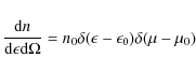
|
(A.1) |
where
|
(A.2) |
Developing the Dirac functions leads to
with
|
(A.4) |
The transform giving
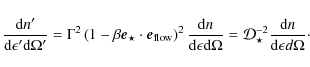
The anisotropic inverse Compton scattering kernel in Dubus et al. (2008) can then be used, with the photon density given in Eq. (A.3) and with the direction given by
For inverse Compton emission by a power-law distribution of
electrons in the Thomson regime, the spectrum in the comoving frame is
given by
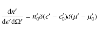
where p is the power-law index and K is a constant. In this case, the spectrum seen by the observer is
|
(A.7) |
so that, using the dot product in Eq. (A.5),
where
For completeness, the orbital separation d is given by
|
(A.9) |
with the semi-major axis
| (A.10) | |||
| (A.11) |
where i is the inclination of the system.
References
- Abdo, A. A., Ackermann, M., Ajello, M., et al. 2009a, ApJ, 701, L123 [NASA ADS] [CrossRef] [Google Scholar]
- Abdo, A. A., Ackermann, M., Ajello, M., et al. 2009b, ApJ, 706, L56 [NASA ADS] [CrossRef] [Google Scholar]
- Abdo, A. A., Ackermann, M., Ajello, M., et al. 2009c, Science, 326, 1512 [NASA ADS] [CrossRef] [PubMed] [Google Scholar]
- Acciari, V. A., Beilicke, M., Blaylock, G., et al. 2008, ApJ, 679, 1427 [NASA ADS] [CrossRef] [Google Scholar]
- Acciari, V. A., Aliu, E., Arlen, T., et al. 2009, ApJ, 700, 1034 [NASA ADS] [CrossRef] [Google Scholar]
- Aharonian, F., Akhperjanian, A. G., Aye, K.-M., et al. 2005a, Science, 309, 746 [NASA ADS] [CrossRef] [PubMed] [Google Scholar]
- Aharonian, F., Akhperjanian, A. G., Aye, K.-M., et al. 2005b, A&A, 442, 1 [Google Scholar]
- Aharonian, F., Akhperjanian, A. G., Bazer-Bachi, A. R., et al. 2006, A&A, 460, 743 [NASA ADS] [CrossRef] [EDP Sciences] [Google Scholar]
- Albert, J., Aliu, E., Anderhub, H., et al. 2006, Science, 312, 1771 [NASA ADS] [CrossRef] [PubMed] [Google Scholar]
- Albert, J., Aliu, E., Anderhub, H., et al. 2009, ApJ, 693, 303 [NASA ADS] [CrossRef] [Google Scholar]
- Anderhub, H., Antonelli, L. A., Antoranz, P., et al. 2009, ApJ, 706, L27 [NASA ADS] [CrossRef] [Google Scholar]
- Aragona, C., McSwain, M. V., Grundstrom, E. D., et al. 2009, ApJ, 698, 514 [NASA ADS] [CrossRef] [Google Scholar]
- Arons, J., & Tavani, M. 1993, ApJ, 403, 249 [NASA ADS] [CrossRef] [Google Scholar]
- Bignami, G. F., Maraschi, L., & Treves, A. 1977, A&A, 55, 155 [NASA ADS] [Google Scholar]
- Bogovalov, S. V., Khangulyan, D. V., Koldoba, A. V., Ustyugova, G. V., & Aharonian, F. A. 2008, MNRAS, 387, 63 [NASA ADS] [CrossRef] [Google Scholar]
- Bosch-Ramon, V., Paredes, J. M., Ribó, M., et al. 2005, ApJ, 628, 388 [NASA ADS] [CrossRef] [Google Scholar]
- Bosch-Ramon, V., Motch, C., Ribó, M., et al. 2007, A&A, 473, 545 [NASA ADS] [CrossRef] [EDP Sciences] [Google Scholar]
- Chernyakova, M., Neronov, A., Aharonian, F., Uchiyama, Y., & Takahashi, T. 2009, MNRAS, 397, 2123 [NASA ADS] [CrossRef] [Google Scholar]
- Chernyakova, M., Neronov, A., & Walter, R. 2006, MNRAS, 372, 1585 [NASA ADS] [CrossRef] [Google Scholar]
- Dermer, C. D., & Schlickeiser, R. 1993, ApJ, 416, 458 [NASA ADS] [CrossRef] [Google Scholar]
- Dermer, C. D., Schlickeiser, R., & Mastichiadis, A. 1992, A&A, 256, L27 [NASA ADS] [Google Scholar]
- Dhawan, V., Mioduszewski, A., & Rupen, M. 2006, in Proc. of the VI Microquasar Workshop: Microquasars and Beyond (MQW6), 52 [Google Scholar]
- Dubus, G. 2006, A&A, 456, 801 [NASA ADS] [CrossRef] [EDP Sciences] [Google Scholar]
- Dubus, G., Cerutti, B., & Henri, G. 2008, A&A, 477, 691 [NASA ADS] [CrossRef] [EDP Sciences] [Google Scholar]
- Dubus, G., Cerutti, B., & Henri, G. 2010, MNRAS, 404, L55 [NASA ADS] [Google Scholar]
- Georganopoulos, M., Kirk, J. G., & Mastichiadis, A. 2001, ApJ, 561, 111 [NASA ADS] [CrossRef] [Google Scholar]
- Hinton, J. A., Skilton, J. L., Funk, S., et al. 2009, ApJ, 690, L101 [NASA ADS] [CrossRef] [Google Scholar]
- Hoffmann, A. D., Klochkov, D., Santangelo, A., et al. 2009, A&A, 494, L37 [NASA ADS] [CrossRef] [EDP Sciences] [Google Scholar]
- Huang, H. H., & Becker, W. 2007, A&A, 463, L5 [NASA ADS] [CrossRef] [EDP Sciences] [Google Scholar]
- Kaufman Bernadó, M. M., Romero, G. E., & Mirabel, I. F. 2002, A&A, 385, L10 [NASA ADS] [CrossRef] [EDP Sciences] [Google Scholar]
- Kennel, C. F., & Coroniti, F. V. 1984, ApJ, 283, 694 [NASA ADS] [CrossRef] [Google Scholar]
- Kishishita, T., Tanaka, T., Uchiyama, Y., & Takahashi, T. 2009, ApJ, 697, L1 [NASA ADS] [CrossRef] [Google Scholar]
- Manchester, R. N., Johnston, S., Lyne, A. G., et al. 1995, ApJ, 445, L137 [NASA ADS] [CrossRef] [Google Scholar]
- Maraschi, L., & Treves, A. 1981, MNRAS, 194, 1P [NASA ADS] [CrossRef] [Google Scholar]
- Martocchia, A., Motch, C., & Negueruela, I. 2005, A&A, 430, 245 [NASA ADS] [CrossRef] [EDP Sciences] [Google Scholar]
- Motch, C., Haberl, F., Dennerl, K., Pakull, M., & Janot-Pacheco, E. 1997, A&A, 323, 853 [NASA ADS] [Google Scholar]
- Pelling, R. M., Paciesas, W. S., Peterson, L. E., et al. 1987, ApJ, 319, 416 [NASA ADS] [CrossRef] [Google Scholar]
- Reig, P., Ribó, M., Paredes, J. M., & Martí, J. 2003, A&A, 405, 285 [NASA ADS] [CrossRef] [EDP Sciences] [Google Scholar]
- Ribó, M., Reig, P., Martí, J., & Paredes, J. M. 1999, A&A, 347, 518 [NASA ADS] [Google Scholar]
- Takahashi, T., Kishishita, T., Uchiyama, Y., et al. 2009, ApJ, 697, 592 [NASA ADS] [CrossRef] [Google Scholar]
- Tavani, M., Arons, J., & Kaspi, V. M. 1994, ApJ, 433, L37 [NASA ADS] [CrossRef] [Google Scholar]
Footnotes
- ... model
![[*]](/icons/foot_motif.png)
- Here, the injected number of fresh particles is kept constant along the orbit whereas the energy density of cooled particles had been kept constant in Dubus et al. (2008). With the energy density constant, the particle distribution varied very little with orbital phase, which highlighted the impact of anisotropic scattering. However, a constant injection in number of particles is probably more realistic (at least for a pulsar wind). It has no noticeable influence on the spectra but it slightly changes the VHE lightcurve from that shown in Dubus et al. (2008). The VHE lightcurve remains compatible with the HESS results.
All Figures
|
|
Figure 1: Geometry of Doppler
boosted emission from a collimated shock pulsar wind nebula. The orbit
is that of LS 5039 (to scale). The comet tail moves away from the
pulsar with a speed |
| Open with DEXTER | |
| In the text | |
|
|
Figure 2: Comparison of the model for LS 5039 described in Sect. 2.3 with observations. Top panel: spectral energy distribution showing the Suzaku 1-10 keV maximum and minimum spectra (Takahashi et al. 2009), the 100 MeV-10 GeV average Fermi spectrum (Abdo et al. 2009b) and the VHE spectra averaged over phases INFC (dark points) and SUPC (grey points) as defined in Aharonian et al. (2006). The model spectra averaged over INFC and SUPC are shown as dark and grey curves. Middle and bottom panels: expected VHE gamma-ray and X-ray orbital modulation compared to the HESS and Suzaku observations. |
| Open with DEXTER | |
| In the text | |
|
|
Figure 3:
Doppler-boosted synchrotron (
|
| Open with DEXTER | |
| In the text | |
|
|
Figure 4:
Same as Fig. 1
but with the corrections due to relativistic motion taken into account.
The flow is assumed to originate at the compact object location with |
| Open with DEXTER | |
| In the text | |
|
|
Figure 5:
Doppler-boosted synchrotron (
|
| Open with DEXTER | |
| In the text | |
|
|
Figure 6:
Doppler-boosted synchrotron (
|
| Open with DEXTER | |
| In the text | |
|
|
Figure A.1: Geometry of the binary + pulsar wind nebula flow system. The calculations assume that the massive star is point-like and that emission in the tail is limited to a small region at the pulsar location. |
| Open with DEXTER | |
| In the text | |
Copyright ESO 2010
Current usage metrics show cumulative count of Article Views (full-text article views including HTML views, PDF and ePub downloads, according to the available data) and Abstracts Views on Vision4Press platform.
Data correspond to usage on the plateform after 2015. The current usage metrics is available 48-96 hours after online publication and is updated daily on week days.
Initial download of the metrics may take a while.