| Issue |
A&A
Volume 516, June-July 2010
|
|
|---|---|---|
| Article Number | A26 | |
| Number of page(s) | 10 | |
| Section | Numerical methods and codes | |
| DOI | https://doi.org/10.1051/0004-6361/200912443 | |
| Published online | 22 June 2010 | |
High-order Godunov schemes for global 3D MHD simulations of accretion disks
I. Testing the linear growth of the magneto-rotational instability
M. Flock1 - N. Dzyurkevich1 - H. Klahr1 - A. Mignone2
1 - Max Planck Institute for Astronomy, Königstuhl 17,
69117 Heidelberg, Germany
2 -
Dipartimento di Fisica Generale, Universitá degli Studi di
Torino, via Pietro Giuria 1, 10125 Torino, Italy
Received 7 May 2009 / Accepted 16 April 2010
Abstract
We assess the suitability of various numerical MHD
algorithms for astrophysical accretion disk simulations with the
PLUTO code. The well-studied linear growth of the
magneto-rotational instability is used as the benchmark test for a
comparison between the implementations within PLUTO and against the ZeusMP code. The results demonstrate
the importance of using an upwind reconstruction of the
electro-motive force (EMF) in the context of a constrained transport scheme, which is consistent with plane-parallel,
grid-aligned flows. In contrast, constructing the EMF from the
simple average of the Godunov fluxes leads to a numerical
instability and the unphysical growth of the magnetic energy. We
compare the results from 3D global calculations using different MHD
methods against the analytical solution for the linear growth of the
MRI, and discuss the effect of numerical dissipation. The
comparison identifies a robust and accurate code configuration that
is vital for realistic modeling of accretion disk processes.
Key words: accretion, accretion disks - magnetohydrodynamics (MHD) - methods: numerical
1 Introduction
It is widely accepted that the magneto-rotational instability (MRI) can be responsible for turbulence in proto-planetary disks, enabling the accretion of the disk material onto the star. The turbulence interacts with the gas-phase chemistry, grain growth and settling, and thermal evolution, which makes the understanding of planet formation a challenge. In particular, the effectiveness of MRI-driven turbulence depends on the ionization degree of the gas (Wardle 1999; Jin 1996; Blaes & Balbus 1994; Gammie 1996; Ilgner & Nelson 2006; Turner et al. 2007; Fleming et al. 2000; Sano et al. 2000). The collisional ionization rate depends on the temperature, which at sufficiently high accretion rates is governed by the dissipation of magnetic fields in the turbulence. Accurately capturing the magnetic energy loss during diffusion and reconnection as heat requires an energy-conserving numerical scheme.
Many classical studies of the magneto-rotational instability (MRI) were conducted with the ideal MHD approach and the local shearing box approximation (Hawley et al. 1995; Sano et al. 2004; Matsumoto & Tajima 1995; Brandenburg et al. 1995; Stone et al. 1996; Hawley et al. 1996), partly reviewed in Balbus & Hawley (1998). However, recent developments have shown that critical questions about turbulence in accretion disks can only be addressed in global simulations (Lyra et al. 2008; Davis et al. 2010; Fromang & Papaloizou 2007; Fromang & Nelson 2009,2006). The majority of the existing codes which can handle global disk simulations are based on Zeus-like finite difference schemes (Hawley 2000; Fromang & Nelson 2009,2006). Thus, it would be beneficial to tackle the open questions with an independent method. A number of investigators have recognized the importance of using conservative Godunov-type upwind schemes rather than non-conservative finite difference algorithms (Fromang et al. 2006; Stone & Gardiner 2005; Mignone et al. 2007), especially for jets and space weather simulations (Groth et al. 2000).
So far, no global calculation has treated temperature changes in the
disk. Some first results in this direction apply the flux-limited
radiation diffusion approach in shearing-box calculations (Flaig et al. 2009; Turner 2004; Hirose et al. 2006; Turner et al. 2002).
The latter use a conservative, cell-centered finite
volume scheme. A major challenge here is to accurately and effectively
monitor and control the evolution of the divergence of the magnetic field,
which should stay at
![]() .
.
Two main approaches for evolving the magnetic field have been
established over the years. The first is the ``constrained
transport'' (CT) method (Evans & Hawley 1988; Stone & Norman 1992; Hawley & Stone 1995; Devore 1991; Brecht et al. 1981). By discretizing the magnetic and electric
vector fields on a staggered mesh, this scheme achieves the important
property of maintaining
![]() to machine accuracy.
Several issues arise in choosing how to adapt the CT method to the
cell-centered discretization used in the Godunov MHD schemes. Constrained
transport Godunov schemes introduced by Dai & Woodward (1998), Ryu et al. (1998), Balsara & Spicer (1999), Komissarov (1999) and Tóth (2000) include
both staggered and cell-centered magnetic fields. The difficulty is
that the staggered field is not well suited for upwind Godunov schemes.
For a staggered field, the
one-dimensional solutions of the Riemann problem for density, momentum
and the energy equation have no direct extension to the upwind fluxes
in the induction equation (Balsara & Spicer 1999).
Londrillo & Del Zanna (2000) and Londrillo & del Zanna (2004) enhanced the CT method to make it
consistent with the one-dimensional solver for plane parallel,
grid-aligned flows. Based on the Harten-Lax-van Leer (HLL) and Roe Riemann solver fluxes, they
proposed a new way to reconstruct the electric fields now called
``upwind CT''. In Londrillo & del Zanna (2004) they followed a similar approach by
using the Hamilton-Jacobi equations to derive the method as proposed in
Kurganov et al. (2001). Further improvements of the CT approach were
introduced in the ATHENA code Gardiner & Stone (2005) and the RAMSES code
(Fromang et al. 2006), both based on the work of Londrillo & del Zanna (2004).
to machine accuracy.
Several issues arise in choosing how to adapt the CT method to the
cell-centered discretization used in the Godunov MHD schemes. Constrained
transport Godunov schemes introduced by Dai & Woodward (1998), Ryu et al. (1998), Balsara & Spicer (1999), Komissarov (1999) and Tóth (2000) include
both staggered and cell-centered magnetic fields. The difficulty is
that the staggered field is not well suited for upwind Godunov schemes.
For a staggered field, the
one-dimensional solutions of the Riemann problem for density, momentum
and the energy equation have no direct extension to the upwind fluxes
in the induction equation (Balsara & Spicer 1999).
Londrillo & Del Zanna (2000) and Londrillo & del Zanna (2004) enhanced the CT method to make it
consistent with the one-dimensional solver for plane parallel,
grid-aligned flows. Based on the Harten-Lax-van Leer (HLL) and Roe Riemann solver fluxes, they
proposed a new way to reconstruct the electric fields now called
``upwind CT''. In Londrillo & del Zanna (2004) they followed a similar approach by
using the Hamilton-Jacobi equations to derive the method as proposed in
Kurganov et al. (2001). Further improvements of the CT approach were
introduced in the ATHENA code Gardiner & Stone (2005) and the RAMSES code
(Fromang et al. 2006), both based on the work of Londrillo & del Zanna (2004).
The second class of MHD methods exclusively uses the cell center discretization.
Here there is no additional staggered grid and
![]() is not automatically forced to vanish.
Solution attempts for this problem were presented by Powell (1994), Powell et al. (1999) or Dedner et al. (2002).
The so called ``eight waves'' method uses the modified MHD equations with specific source
terms and allows magnetic monopoles to appear as an additional
is not automatically forced to vanish.
Solution attempts for this problem were presented by Powell (1994), Powell et al. (1999) or Dedner et al. (2002).
The so called ``eight waves'' method uses the modified MHD equations with specific source
terms and allows magnetic monopoles to appear as an additional
![]() mode in the classical seven-mode Riemann fan.
A further development is the hyperbolic cleaning method of
Dedner et al. (2002). Here the conservative form of the MHD system is
preserved by introducing a time-dependent wave equation which dampens
the monopoles. Whether these technique sufficiently removes
mode in the classical seven-mode Riemann fan.
A further development is the hyperbolic cleaning method of
Dedner et al. (2002). Here the conservative form of the MHD system is
preserved by introducing a time-dependent wave equation which dampens
the monopoles. Whether these technique sufficiently removes
![]() strongly depends on the problem and for MHD turbulence this was
never actually shown.
strongly depends on the problem and for MHD turbulence this was
never actually shown.
The PLUTO code is a conservative multi-dimensional and multi-geometry code that can be applied to relativistic or non-relativistic MHD or pure HD flows. The ability to switch between several different numerical modules in PLUTO allows us to test and compare a range of different methods, such as cell-centered and CT, and choose those giving the best convergence and stability properties, defining a consistent algorithm. For example, the code offers the possibility of using the Riemann solvers of Roe, Harten-Lax-van Leer Discontinuities (HLLD), Harten-Lax-van Leer Contact (HLLC), HLL and Lax-Friedrichs (Rusanov) types. The PLUTO code has successfully reproduced a series of standard MHD tests, including the rotating shock-tube, the fast rotor and the blast wave solution (Mignone et al. 2007). The methods are reviewed in Balsara (2004) and Mignone & Bodo (2008).
In this paper we investigate the behavior of various MHD algorithms in 3D global accretion disk calculations using cylindrical coordinates. The results from the PLUTO Godunov code are compared with those from ZeusMP, which represents a certain class of widespread finite difference codes. ZeusMP (Stone & Norman 1992; Hayes et al. 2006) uses a classical staggered discretization of the magnetic and electric vector fields (MoC-CT). We use the ZeusMP version 1b, which has already been applied successfully to 3D global MHD accretion disk calculations (Fromang & Nelson 2006; Dzyurkevich et al. 2010). We set up identical models in the two codes, and examine the performance of the different numerical schemes by comparing the growth of the MRI with the expectations from linear analysis. At the same time, unphysical results are easily discovered by comparison with linear analysis. In Sect. 2 we describe the differences between the numerical schemes of ZEUS and PLUTO. Sect. 3 presents the disk model and the measurement methods. In Sect. 4 we show the results of the inter-code comparison. The convergence properties of the finally identified best suited algorithm are investigated in Sect. 5. Conclusions and an outlook are given in Sect. 6.
2 Numerics
2.1 MHD equations
The equations of ideal magnetohydrodynamics written in conservative form as
implemented in Godunov schemes are
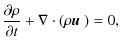
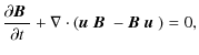
and
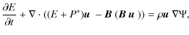
where
2.1.1 ZEUS
The momentum equation is solved by ZeusMP in a non-conservative way,
Density and pressure are stored at the cell center, but as the vector components of velocity and magnetic fields are stored at the grid interfaces, fluxes can be calculated directly in ZEUS. The scheme is second order in space and first order in time in regions between shocks. Although there are no shocks in our runs, we are aware of the anti-diffusive behavior of ZEUS for shocks as it was pointed out in Falle (2002) when using ZEUS without artificial viscosity.
In Sect. 5, we therefore present a test-run with ZEUS including the usual amount of artificial viscosity as it is used in global simulations.
2.1.2 PLUTO
Contrary to Zeus-type finite difference schemes, a Godunov type scheme follows a conservative ansatz. In general all quantities are stored at the cell center. Only for the CT MHD method there is an additional staggered magnetic field. The second order Runge-Kutta (RK) iterator is employed with a CFL about 0.25. Prior to flux calculation, variables are reconstructed at the grid interface, which implies interpolation with a limited slope. The resulting two different states at the interfaces allow us to solve the Riemann problem, which is the main feature of a Godunov code. We tested the different MHD Riemann solvers of Roe (Cargo & Gallice 1997), HLLD (Miyoshi & Kusano 2005), HLL and Lax-Friedrichs Rusanov in our inter-code comparison. The difference is the number of wave characteristics that are used by each solver. Harten-Lax-van Leer and Lax-Friedrichs solver use the fast magneto-sonic wave characteristic as maximal signal velocity. Harten-Lax-van Leer Discontinuities solver additionally includes the Alfvén wave characteristic and the contact discontinuity. The Roe solver follows all seven MHD waves, including the slow magneto-sonic characteristic. We note that compared to the HLLD and Roe solver, the ZEUS code is four to six times faster. This factor appears because of the two predictor and corrector steps in the Runge-Kutta time integration and the calculation of the different fluxes in the Riemann solver.
![\begin{figure}
\par\includegraphics[width=9cm,clip]{12443fg1.ps}
\end{figure}](/articles/aa/full_html/2010/08/aa12443-09/img24.png)
|
Figure 1:
Analytical growth rate plotted for different qr (solid to
dash-doted lines). Triangles present the measured MRI growth rates from our simulation with
initial axisymmetric white noise disturbance from model
|
| Open with DEXTER | |
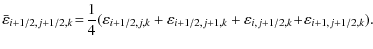
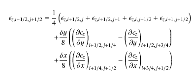
2.2 Constrained transport EMF reconstruction in PLUTO
In the CT approach, the staggered components of B are evolved as
surface averaged quantities and are updated using
Stokes' theorem. This requires constructing a line-averaged electric
field along the face edges using some sort of reconstruction or
averaging technique from the face centers, where different EMF
components are usually available as face-centered upwind Godunov fluxes.
As was already mentioned, it is difficult to represent the solenoidality of magnetic fields correctly in Godunov schemes.
For the constrained transport we will concentrate on three different EMF reconstruction methods.
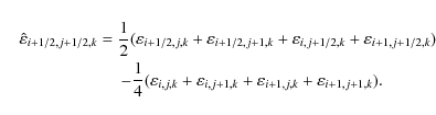
The first method, here called ACT, describes the arithmetic average of the face-centered
EMF's obtained by the
upwind fluxes in the induction equation (Balsara & Spicer 1999) presented in Fig. 1,
|
(6) |
This CT algorithm does not reproduce the correct solution for plane-parallel, grid-aligned flows (Gardiner & Stone 2005). In this case, considering the i-direction, one obtains
| (7) |
in contrast to the correct solution, which is simply
with
and
Both methods,
Table 1: Initial parameter of global setup.
Table 2: MRI growth rates measured for models with 4 and 8 MRI modes (n=4,8).
3 Linear MRI in a global disk
The analytical description of the the linear stage of MRI has been given by Balbus & Hawley (1991). Local shearing box simulations have confirmed the analytical expectation of the linear MRI growth (Hawley et al. 1995; Brandenburg et al. 1995). Global simulations and also the nonlinear evolution of the MRI was presented in Hawley & Balbus (1991). Our simplified setup here is representative for a global proto-planetary disk and made for a modest radial domain.
3.1 Global setup
We use cylindrical coordinates in our models with the notation
|
(8) |
with the angular frequency
3.2 Physical limits of the MRI growth rate
Before using the ideal growth rate as a comparison value,
the processes limiting the growth rate in the linear MRI for a real physical
system have to be considered. When the magneto-rotational instability sets in, the
magnetic fields are amplified with
![]() until they reach saturation.
As mentioned in Hawley & Balbus (1991), the absolute limit of the growth rate
for ideal MHD is given for the zero radial wave vectors qr = 0 with the
normalized wave vector qz,
until they reach saturation.
As mentioned in Hawley & Balbus (1991), the absolute limit of the growth rate
for ideal MHD is given for the zero radial wave vectors qr = 0 with the
normalized wave vector qz,
| (9) |
with the Alfvén speed
The additional effects reducing the MRI growth rate are viscous and resistive dissipation (Pessah & Chan 2008).
For the MRI, the numerical dissipation is the reason why we need some minimal amount of grid cells. Hawley et al. (1995) claim to need at least five grid cells per fastest growing mode for ZEUS to correctly resolve the MRI mode. For the inter-code comparison we used the setup described in Sect. 3.1 with a vertical magnetic field for n=4 and n=8. Then the total resolution of 64 gives 16 grid cells per fastest growing mode, which is enough even for very diffuse solvers. For a better differentiation between the code configurations we include also a weaker vertical magnetic field with n=8, because then only 8 cells per mode are available. Besides resolution and the kind of Riemann solver the order in the reconstruction step also has an impact on the dissipation.
3.3 Measurement method
In Fig. 2 we present the exponential growth of the fastest MRI mode for Br. The slope directly gives us the MRI growth rate. The black lines show the growth for each radial location. Time is given in local orbits. Most radial slices plotted in Fig. 2 show a growth rate close to the analytical limit (see dashed line in Fig. 2). The inner annuli (R=2, red line in Fig. 2) reach non-linear amplitudes first (Fig. 2), producing disturbances that propagate outward and affect the development of the slower-growing linear modes in annuli farther away from the star (R=3, blue line in Fig. 2). As a result the annuli near R=3 grow faster than indicated by the linear analysis and only annuli at R=2 show the predicted behavior. In the following sections the growth rate is calculated as the time average between 1 and 1.5 local orbits.
![\begin{figure}
\hspace{0.6cm}%
\par\includegraphics[width=9cm,clip]{12443fg2a.ps}\vspace*{2.5mm}
\includegraphics[width=9cm,clip]{12443fg2b.ps}
\end{figure}](/articles/aa/full_html/2010/08/aa12443-09/img78.png)
|
Figure 2:
Maximal amplitude growth of the critical MRI mode plotted for
the 42 radial slices between radii R=2 (red line) and R=3 (blue line) for local and inner orbits. The setup is constructed to excite the mode
with
|
| Open with DEXTER | |
4 Inter-code comparison
The models and results of the growth rate for the inter-code comparison are summarized in Table 2.
Here the growth rate values
![]() are averaged over radius and time, as described in Sect. 3.3.
Growth rates higher than the mean analytical value or its
fluctuations are marked in red.
The statistical error is estimated from the radial fluctuation in the growth rate
(Figs. 4, 6 and 9).
are averaged over radius and time, as described in Sect. 3.3.
Growth rates higher than the mean analytical value or its
fluctuations are marked in red.
The statistical error is estimated from the radial fluctuation in the growth rate
(Figs. 4, 6 and 9).
4.1 Magnetic-energy evolution
![\begin{figure}
\hspace{0.6cm}
\par\includegraphics[width=9cm,clip]{12443fg3a.ps}\vspace*{2.5mm}
\includegraphics[width=9cm,clip]{12443fg3b.ps}
\end{figure}](/articles/aa/full_html/2010/08/aa12443-09/img80.png)
|
Figure 3: Radial magnetic energy integrated for the total domain for n=4 ( top) and n=8 ( bottom) with upwind CT (solid line), Powell 8-wave (dashed line) and arithmetic CT (dotted line). The values are normalized over the initial orbital kinetic energy. After the initial disturbance, the growth of critical mode dominates and there is a linear MRI region visible between two and eight inner orbits. For HLLD and Roe, the arithmetic CT shows a growth stronger then MRI until five inner orbits, caused by a numerical instability. Harten-Lax-van Leer and TVDLF have a much lower growth because both methods are viscous and do not resolve the critical mode for the adopted resolution. |
| Open with DEXTER | |
The growth of the magnetic field due to the excitation
of the critical mode dominates at two inner orbits and
the linear growth regime occurs. Figure 3 shows the radial magnetic-energy evolution
![]() for the n=4 and n=8 mode runs (see Table 2). In the
n=8 mode setup we can clearly distinguish
three different families of evolution.
The first family consists of Roe and HLLD solver in combination with ACT (red
colors in Table 2). If the slope is steeper, the analytical prediction is indicating a numerical problem.
Second is the Lax-Friedrichs and HLL Riemann solver. They
always show the slowest growth in energy, independent of the chosen MHD
method. The third family consists of the HLLD and Roe solvers with upwind CT and
the 8-wave method. Their results are the most similar to ZEUS. Below, we will compare the families in detail.
for the n=4 and n=8 mode runs (see Table 2). In the
n=8 mode setup we can clearly distinguish
three different families of evolution.
The first family consists of Roe and HLLD solver in combination with ACT (red
colors in Table 2). If the slope is steeper, the analytical prediction is indicating a numerical problem.
Second is the Lax-Friedrichs and HLL Riemann solver. They
always show the slowest growth in energy, independent of the chosen MHD
method. The third family consists of the HLLD and Roe solvers with upwind CT and
the 8-wave method. Their results are the most similar to ZEUS. Below, we will compare the families in detail.
4.2 The arithmetic CT plus HLLD and Roe
For the ACT in combination with HLLD & Roe solvers the growth of the magnetic energy
overshoots the analytical expectation for MRI growth (Table 2, Figs. 3, 4).
A numerical instability dominates, which shows up in the fastest-growing mode
that has a vertical wavelength shorter than predicted from linear analysis
of MRI.
In Fig. 5 we plotted the growth rate for each radial slice, calculated from 1
to 1.5 local orbits. Roe and HLLD show the same unphysical high radial
variations in growth rate, which locally exceeds the analytical limit.
The instability generates a ``checkerboard'' pattern in physical space for all
variables (see example for ![]() in Fig. 5).
Numerical instabilities rooted in the treatment of the Alfvén
wave were already predicted by Miyoshi & Kusano (2008).
They write that it is commonly known that highly accurate Riemann
solvers for the Euler equations sometimes encounter multi-dimensional
numerical instabilities at high mach
numbers such as the ``carbuncle'' instability that may be related to
the
resolution of the contact wave (Robinet et al. 2000).
in Fig. 5).
Numerical instabilities rooted in the treatment of the Alfvén
wave were already predicted by Miyoshi & Kusano (2008).
They write that it is commonly known that highly accurate Riemann
solvers for the Euler equations sometimes encounter multi-dimensional
numerical instabilities at high mach
numbers such as the ``carbuncle'' instability that may be related to
the
resolution of the contact wave (Robinet et al. 2000).
The reason for the ``checkerboard'' instability is based on the inconsistent EMF reconstruction of ACT for a plane-parallel flow as it is described in Sect. 2.2. The Roe and HLLD solvers include the Alfvén characteristics accurately and evolve the disturbances independently of the resolution (see Fig. 7a). The HLL and TVDLF solver do not include the Alfvén characteristics. For moderate resolutions they present correct results in combination with ACT because the ``checkerboard'' instability is suppressed by numerical dissipation. However, at higher resolutions the numerical instability occurs here as well (see Fig. 7b). For HLL and TVDLF it depends on the dissipation to resolve the numerical instability related to the Alfvén wave. For the Roe and HLLD solver the instability is present for basically any resolution.
![\begin{figure}
\hspace{0.6cm}%
\par\includegraphics[width=9cm,clip]{12443fg4a.ps}\vspace*{2.5mm}
\includegraphics[width=9cm,clip]{12443fg4b.ps}
\end{figure}](/articles/aa/full_html/2010/08/aa12443-09/img82.png)
|
Figure 4: Local growth rate for n=4 ( top) and n=8 ( bottom) with arithmetic CT. For HLLD and Roe the local growth rate exceeds the analytical limit and shows unphysical spatial variations. The problem does not affect the HLL and TVDLF solver at moderate resolution. Harten-Lax-van Leer (green) and TVDLF show exact the same results. |
| Open with DEXTER | |
![\begin{figure}
\hspace{0.6cm}%
\par\includegraphics[width=9cm,clip]{12443fg5a.ps...
...g5b.ps}\vspace*{3mm}
\includegraphics[width=9cm,clip]{12443fg5c.ps}
\end{figure}](/articles/aa/full_html/2010/08/aa12443-09/img83.png)
|
Figure 5: Contour plot of the azimuthal magnetic field for arithmetic CT (top), UCT ( middle) and ZEUS (bottom). For the arithmetic CT, the ``checkerboard'' instability dominates. For UCT and ZEUS the n=4 is most prominent. A change from blue to red indicates a change of sign in the magnetic field. This snap-shot of the magnetic field is taken after eight inner orbits. |
| Open with DEXTER | |
4.3 Upwind CT and 8-wave
With the upwind CT EMF reconstruction described in Sect. 2.2, there is no more ``checkerboard'' pattern visible.
Figure 5 presents a contour plot of the azimuthal magnetic field after eight inner orbits.
The HLLD solver with upwind CT and ZEUS shows four evolving modes.
Figure 6 shows the small difference of local growth rates between ``8-waves'' (8W) and upwind CT (UCT
&
![]() ). One sees that the choice of the Riemann solver has a stronger effect on the
growth rate than the MHD method. Thus, the solution in family ``3'' appears
to be the proper choice for MRI simulations.
). One sees that the choice of the Riemann solver has a stronger effect on the
growth rate than the MHD method. Thus, the solution in family ``3'' appears
to be the proper choice for MRI simulations.
![\begin{figure}
\hspace{0.6cm}
\par\includegraphics[width=9cm,clip]{12443fg6a.ps}\\ \vspace*{3mm}
\includegraphics[width=9cm,clip]{12443fg6b.ps}
\end{figure}](/articles/aa/full_html/2010/08/aa12443-09/img85.png)
|
Figure 6:
Local growth rate for n=4 (top) and n=8 (bottom) with upwind CT (solid line),
|
| Open with DEXTER | |
4.4 The resolution of the most unstable mode
![\begin{figure}
\hspace{0.6cm}%
\par\includegraphics[width=9cm,clip]{12443fg7a.ps}\\ \vspace*{3mm}
\includegraphics[width=9cm,clip]{12443fg7b.ps}
\end{figure}](/articles/aa/full_html/2010/08/aa12443-09/img86.png)
|
Figure 7:
Top: contour plot of radial magnetic field for n=8 mode low resolution run. Even with a
resolution of
|
| Open with DEXTER | |
In the case of four MRI modes and 64 grid cells in the vertical direction, the resolution in the
Z direction is sufficient for all Riemann
solvers to resolve the critical mode, e.g.
![]() .
The HLLD solver, Roe and ZEUS show the highest growth rate followed by TVDLF and HLL.
The models for n=8 are summarized in Table 2 and Fig. 6.
The resolution of eight grid cells per critical mode is not sufficient to resolve the MRI mode.
Here, growth rates are significantly reduced for HLL and TVDLF solvers because
they can only resolve the slower growing 4 mode for the used resolution.
ZEUS and the MHD Riemann solver Roe and HLLD resolve seven modes.
The additional Alfvén characteristics included in the HLLD solver lead
effectively to lower numerical dissipation.
Figure 8 shows a contour plot of the radial magnetic field after seven inner orbits for
the HLLD solver, ZEUS and the HLL solver.
The ZEUS code shows an MRI pattern very close to those of HLLD and Roe.
.
The HLLD solver, Roe and ZEUS show the highest growth rate followed by TVDLF and HLL.
The models for n=8 are summarized in Table 2 and Fig. 6.
The resolution of eight grid cells per critical mode is not sufficient to resolve the MRI mode.
Here, growth rates are significantly reduced for HLL and TVDLF solvers because
they can only resolve the slower growing 4 mode for the used resolution.
ZEUS and the MHD Riemann solver Roe and HLLD resolve seven modes.
The additional Alfvén characteristics included in the HLLD solver lead
effectively to lower numerical dissipation.
Figure 8 shows a contour plot of the radial magnetic field after seven inner orbits for
the HLLD solver, ZEUS and the HLL solver.
The ZEUS code shows an MRI pattern very close to those of HLLD and Roe.
With the two different setups (n=4 & n=8) we can conclude that the HLL and TVDLF Riemann solver need at least 16 grid cells per mode to resolve the fastest growing MRI mode correctly. The HLLD and Roe solver can resolve the mode starting with 10 grid cells per mode.
![\begin{figure}
\par\includegraphics[width=9cm,clip]{12443fg8a.ps}\vspace*{2.8mm}...
...8mm}
\includegraphics[width=9cm,clip]{12443fg8c.ps}\vspace*{-3.5mm}
\end{figure}](/articles/aa/full_html/2010/08/aa12443-09/img88.png)
|
Figure 8: Contour plot of the radial magnetic field in code units for the HLLD solver ( top), ZEUS ( middle) and HLL solver ( bottom). After seven inner orbits the inner radial part breaks into a nonlinear regime. |
| Open with DEXTER | |
4.5 The role of the reconstruction method for primitive variables
The reconstruction of the states at the interface is the main source of dissipation in Godunov schemes (see Sect. 2). In this subsection we test the third order piece-wise parabolic method (PPM) by Collela (1984) and compare the results with the piece-wise linear reconstruction method (PLM) used in the previous sections.
![\begin{figure}
\par\includegraphics[width=9cm,clip]{12443fg9a.ps}\vspace*{3mm}
\includegraphics[width=9cm,clip]{12443fg9b.ps}
\end{figure}](/articles/aa/full_html/2010/08/aa12443-09/img89.png)
|
Figure 9: Growth rate of MRI for PPM (dashed line) and PLM (solid line). For the Lax-Friedrichs solver the PPM interpolation leads to growth rates closer to the analytic solution, which is due to lower numerical dissipation. Differences between HLLD and Roe solvers are less prominent. |
| Open with DEXTER | |
Nevertheless, using an order of spatial reconstruction beyond the order of time integration can lead to anti-diffusive behavior. This can artificially generate or amplify magnetic fields, as shown in Falle (2002). Therefore one should avoid to compensate the dissipation of the method with high order reconstruction and choose instead a high-order Riemann solver as HLLD or Roe.
Table 3: Growth rates for the resolution tests with initial 4 mode (4M) and white noise perturbations (WN).
5 High-resolution comparison
The models in our convergence test are summarized in Table 3. We adopt the n=4 model with 2 different initial perturbations, white noise and a n=4 perturbation in velocity.
5.1 The role of initial perturbation
Usually the global 3D simulation of a disk starts with white-noise velocity
perturbation. This initial configuration is least presumptive in the
evolution.
All three components of the velocity are
perturbed, and a large range of MRI modes is excited. Due to the excitation
of several radial modes, the growth rate of the MRI is below the analytical value
![]() as presented in Fig. 1.
Nevertheless, such a test allows us to compare the codes in the most
complete global setup, not precluding specific unstable modes.
Another approach is to exclusively perturb the radial velocity with only one chosen mode, for example
as presented in Fig. 1.
Nevertheless, such a test allows us to compare the codes in the most
complete global setup, not precluding specific unstable modes.
Another approach is to exclusively perturb the radial velocity with only one chosen mode, for example
![]() where H is the vertical size of the box.
In combination with an initial magnetic field of
Bz=0.05513/4, a pure clean n=4 mode
will be exited. Such a perturbation is highly artificial, yet the purpose
is to approach the analytical value for a linear MRI growth of
where H is the vertical size of the box.
In combination with an initial magnetic field of
Bz=0.05513/4, a pure clean n=4 mode
will be exited. Such a perturbation is highly artificial, yet the purpose
is to approach the analytical value for a linear MRI growth of
![]() .
As our tests are performed in the global framework, there is still the effect of
radial change in orbital frequency, leading to local variation in the growth
rate. Therefore we choose for our analysis one
annulus close to R=2, where the growth rate seems to be least affected
(see Fig. 2).
.
As our tests are performed in the global framework, there is still the effect of
radial change in orbital frequency, leading to local variation in the growth
rate. Therefore we choose for our analysis one
annulus close to R=2, where the growth rate seems to be least affected
(see Fig. 2).
5.1.1 White noise perturbation
In the runs
![]() ,
,
![]() ,
,
![]() we used axis-symmetric white noise for the radial and vertical
velocity perturbations.
Table 3 summarizes the maximum growth rate for both initial perturbations.
For
we used axis-symmetric white noise for the radial and vertical
velocity perturbations.
Table 3 summarizes the maximum growth rate for both initial perturbations.
For
![]() ,
,
![]() and
and
![]() ,
the linear MRI tops at a growth rate
around 0.7 for higher resolutions.
Only for the lowest resolution we can clearly see a lower growth rate, which stresses our earlier conclusion that
8 grid cells per critical mode are not sufficient. For this resolution the
HLLD with the PPM reconstruction has the most similar behavior to ZEUS.
In this set of tests, the reason for not reaching the analytical value of
,
the linear MRI tops at a growth rate
around 0.7 for higher resolutions.
Only for the lowest resolution we can clearly see a lower growth rate, which stresses our earlier conclusion that
8 grid cells per critical mode are not sufficient. For this resolution the
HLLD with the PPM reconstruction has the most similar behavior to ZEUS.
In this set of tests, the reason for not reaching the analytical value of
![]() is a physical one.
The limit of the growth rate is set by the various occurring radial modes which are excited in case of the
white noise perturbation (see Fig. 1).
With increasing resolution, smaller and smaller radial modes are resolved
and no convergence can be achieved, because the setup changes.
The details of the behavior of both codes for the low resolution
and the white noise setup are available in Fig. 11.
is a physical one.
The limit of the growth rate is set by the various occurring radial modes which are excited in case of the
white noise perturbation (see Fig. 1).
With increasing resolution, smaller and smaller radial modes are resolved
and no convergence can be achieved, because the setup changes.
The details of the behavior of both codes for the low resolution
and the white noise setup are available in Fig. 11.
![\begin{figure}
\par\includegraphics[width=9cm,clip]{12443fg10a.ps}\vspace*{2.5mm}
\includegraphics[width=9cm,clip]{12443fg10b.ps}\vspace*{-2mm}
\end{figure}](/articles/aa/full_html/2010/08/aa12443-09/img102.png)
|
Figure 10:
Convergence for the white noise ( top) and single 4 mode perturbation setup ( bottom).
For the single 4 mode perturbation the growth rates exhibit a quick convergence to the analytical limit
|
| Open with DEXTER | |
5.1.2 Initial 4 mode perturbation
Only with this artificial setup can we assure that we have initial
perturbations independent on resolution, which is necessary for convergence
studies.
In the runs
![]() and
and
![]() we avoid the
excitation of MRI waves
we avoid the
excitation of MRI waves
![]() by choosing
by choosing
![]() for initial
disturbance without any radial dependence.
In Fig. 10 we plot the growth-rate evolution for a specific radial point
near
for initial
disturbance without any radial dependence.
In Fig. 10 we plot the growth-rate evolution for a specific radial point
near
![]() ,
which presents the region of the smoothest linear growth regime
compared to the outer annulus at R=3 (Fig. 2).
Table 3 summarizes the maximum growth rate measured in Fig. 10.
Both the codes
,
which presents the region of the smoothest linear growth regime
compared to the outer annulus at R=3 (Fig. 2).
Table 3 summarizes the maximum growth rate measured in Fig. 10.
Both the codes
![]() and
and
![]() converge on the analytical limit of
converge on the analytical limit of
![]() .
It is interesting to note that for the ultimately lowest resolution the growth rates from
.
It is interesting to note that for the ultimately lowest resolution the growth rates from
![]() in combination with the second order piece-wise linear reconstruction
method (PLM)
is lower then the
in combination with the second order piece-wise linear reconstruction
method (PLM)
is lower then the
![]() value.
The reason for this is buried inside the PLM method, which causes a
higher dissipation compared to PPM (Fig. 11 dash-dotted line). Additionally, we
did not use artificial viscosity in ZEUS, which one would usually switch
on in a global simulation and which reduces the growth rate (Fig. 11 dashed
line).
The dashed red line in Fig. 10 shows the growth rate for PLUTO with the third order
convex-eno reconstruction (Del Zanna & Bucciantini 2002). The growth rate is
closer to
value.
The reason for this is buried inside the PLM method, which causes a
higher dissipation compared to PPM (Fig. 11 dash-dotted line). Additionally, we
did not use artificial viscosity in ZEUS, which one would usually switch
on in a global simulation and which reduces the growth rate (Fig. 11 dashed
line).
The dashed red line in Fig. 10 shows the growth rate for PLUTO with the third order
convex-eno reconstruction (Del Zanna & Bucciantini 2002). The growth rate is
closer to
![]() for the doubled resolution (green lines).
for the doubled resolution (green lines).
The highest resolution run is almost the limit on even the fastest computers; it was calculated on the Blue Gene/P taking nearly 50 000 CPU h for 11 inner orbits. In contrast, global simulations on viscous times-scales need 10 000 orbits.
![\begin{figure}
\par\includegraphics[width=9cm,clip]{12443fg11.ps}
\end{figure}](/articles/aa/full_html/2010/08/aa12443-09/img106.png)
|
Figure 11:
Four mode perturbation setup for different reconstruction methods. For
the lowest resolution, the base dissipation of the scheme becomes important
for the growth rate value. The convex eno reaches the growth rate value as
for the
|
| Open with DEXTER | |
6 Conclusions
We have identified a robust and accurate Godunov scheme for 3D MHD simulations in curvilinear coordinate systems through demonstrating convergence and stability for the well studied linear growth phase of the MRI. Crucially, the scheme uses a constrained transport reconstruction of the EMF's which is consistent with the plane-parallel, grid-aligned flow, which is found in Keplerian flows in curvilinear coordinates. By contrast, a four-point arithmetic average CT method leads to the growth of a ``checkerboard'' numerical instability. The HLLD and Roe Riemann solvers present this instability independent of resolution. Both solvers treat the Alfvén characteristics in the Riemann fan. The numerical instability is obviously connected to the Alfvén wave (Miyoshi & Kusano 2008). Harten-Lax-van Leer and Lax-Friedrichs do not resolve the instability for moderate resolutions. The results of our inter-code comparison and convergence tests stress the importance of properly treating the Alfvén characteristics in Riemann solvers for flows driven by the MRI. Alongside loop advection (Gardiner & Stone 2008), the linear evolution of the MRI is a key test problem. We measured the linear MRI growth rates in both the finite difference code Zeus and the Godunov code PLUTO with several different Riemann solvers. More than eight grid cells per wavelength are needed to correctly evolve the MRI mode in both codes. The numerical dissipation is greater with the Lax-Friedrichs and HLL solvers than with the finite difference scheme of ZEUS, owing to the reconstruction of the interface states in the former. The HLLD and Roe Riemann solvers achieve a lower dissipation by including additional MHD characteristics. During the linear growth, the HLLD and Roe solvers show results similar to the finite difference scheme ZEUS for the same order of accuracy and resolution. In addition, the HLLD solver yields an evolution very similar to that obtained with the Roe solver, despite the neglect of the slow magneto-sonic characteristic. A consistent upwind EMF reconstruction in combination with the HLLD Riemann solver gives a consistent, conservative and efficient scheme for our future 3D global MHD calculations of accretion disks. In a follow-up work we will perform and study the non-linear MRI evolution including resistive MHD.
AcknowledgementsWe thank Udo Ziegler for very useful discussions about the upwind constrained transport. We also thank Neal Turner, Ralf Kissmann, Thomas Henning and Matthias Griessinger for comments on the manuscript. H. Klahr, N. Dzyurkevich and M. Flock have been supported in part by the Deutsche Forschungsgemeinschaft DFG through grant DFG Forschergruppe 759 The Formation of Planets: The Critical First Growth Phase. Parallel computations have been performed on the PIA cluster of the Max-Planck Institute for Astronomy Heidelberg located at the computing center of the Max-Planck Society in Garching.
References
- Balbus, S. A., & Hawley, J. F. 1991, ApJ, 376, 214 [NASA ADS] [CrossRef] [Google Scholar]
- Balbus, S. A., & Hawley, J. F. 1998, Rev. Mod. Phys., 70, 1 [Google Scholar]
- Balsara, D. S. 2004, ApJS, 151, 149 [NASA ADS] [CrossRef] [Google Scholar]
- Balsara, D. S., & Spicer, D. S. 1999, J. Comput. Phys., 149, 270 [Google Scholar]
- Blaes, O. M., & Balbus, S. A. 1994, ApJ, 421, 163 [NASA ADS] [CrossRef] [Google Scholar]
- Brandenburg, A., Nordlund, A., Stein, R. F., & Torkelsson, U. 1995, ApJ, 446, 741 [NASA ADS] [CrossRef] [Google Scholar]
- Brecht, S. H., Lyon, J., Fedder, J. A., & Hain, K. 1981, Geophys. Res. Lett., 8, 397 [NASA ADS] [CrossRef] [Google Scholar]
- Cargo, P., & Gallice, G. 1997, J. Comput. Phys., 136, 446 [NASA ADS] [CrossRef] [Google Scholar]
- Dai, W., & Woodward, P. R. 1998, ApJ, 494, 317 [NASA ADS] [CrossRef] [Google Scholar]
- Davis, S. W., Stone, J. M., & Pessah, M. E. 2010, ApJ, 713, 52 [NASA ADS] [CrossRef] [Google Scholar]
- Dedner, A., Kemm, F., Kröner, D., et al. 2002, J. Comput. Phys., 175, 645 [Google Scholar]
- Del Zanna L., & Bucciantini N. 2002, A&A, 390, 1177 [NASA ADS] [CrossRef] [EDP Sciences] [Google Scholar]
- Devore, C. R. 1991, J. Comput. Phys., 92, 142 [NASA ADS] [CrossRef] [MathSciNet] [Google Scholar]
- Dzyurkevich, N., Flock, M., Turner, N. J., Klahr, H., & Henning, Th. 2010, A&A, 515, A70 [NASA ADS] [CrossRef] [EDP Sciences] [Google Scholar]
- Evans, C. R., & Hawley, J. F. 1988, ApJ, 332, 659 [Google Scholar]
- Falle, S. A. E. G. 2002, ApJ, 577, L123 [NASA ADS] [CrossRef] [Google Scholar]
- Flaig, M., Kissmann, R., & Kley, W. 2009, MNRAS, 282 [Google Scholar]
- Fleming, T. P., Stone, J. M., & Hawley, J. F. 2000, ApJ, 530, 464 [NASA ADS] [CrossRef] [Google Scholar]
- Fromang, S., & Nelson, R. P. 2006, A&A, 457, 343 [NASA ADS] [CrossRef] [EDP Sciences] [MathSciNet] [Google Scholar]
- Fromang, S., & Nelson, R. P. 2009, A&A, 496, 597 [NASA ADS] [CrossRef] [EDP Sciences] [Google Scholar]
- Fromang, S., & Papaloizou, J. 2007, A&A, 476, 1113 [NASA ADS] [CrossRef] [EDP Sciences] [Google Scholar]
- Fromang, S., Hennebelle, P., & Teyssier, R. 2006, A&A, 457, 371 [NASA ADS] [CrossRef] [EDP Sciences] [Google Scholar]
- Gammie, C. F. 1996, ApJ, 457, 355 [NASA ADS] [CrossRef] [Google Scholar]
- Gardiner, T. A., & Stone, J. M. 2005, J. Comput. Phys., 205, 509 [Google Scholar]
- Gardiner, T. A., & Stone, J. M. 2008, J. Comput. Phys., 227, 4123 [NASA ADS] [CrossRef] [Google Scholar]
- Groth C. P. T., De Zeeuw D. L., Gombosi T. I., & Powell K. G. 2000, J. Geophys. Res., 105, 25053 [Google Scholar]
- Hawley, J. F. 2000, ApJ, 528, 462 [NASA ADS] [CrossRef] [Google Scholar]
- Hawley, J. F., & Balbus, S. A. 1991, ApJ, 376, 223 [NASA ADS] [CrossRef] [Google Scholar]
- Hawley, J. F., & Stone, J. M. 1995, Comp. Phys. Comm., 89, 127 [Google Scholar]
- Hawley, J. F., Gammie, C. F., & Balbus, S. A. 1995, ApJ, 440, 742 [NASA ADS] [CrossRef] [Google Scholar]
- Hawley, J. F., Gammie, C. F., & Balbus, S. A. 1996, ApJ, 464, 690 [NASA ADS] [CrossRef] [Google Scholar]
- Hayes, J. C., Norman, M. L., Fiedler, R. A., et al. 2006, ApJS, 165, 188 [NASA ADS] [CrossRef] [Google Scholar]
- Hirose S., Krolik J. H., & Stone J. M. 2006, ApJ, 640, 901 [NASA ADS] [CrossRef] [Google Scholar]
- Ilgner, M., & Nelson, R. P. 2006, A&A, 445, 205 [NASA ADS] [CrossRef] [EDP Sciences] [Google Scholar]
- Jin, L. 1996, ApJ, 457, 798 [NASA ADS] [CrossRef] [Google Scholar]
- Komissarov, S. S. 1999, MNRAS, 303, 343 [NASA ADS] [CrossRef] [Google Scholar]
- Kurganov, A., Noelle, S., & Petrova, G. 2001, J. Sci. Comput., 23, 707 [Google Scholar]
- Londrillo, P., & Del Zanna, L. 2000, ApJ, 530, 508 [NASA ADS] [CrossRef] [Google Scholar]
- Londrillo, P., & del Zanna, L. 2004, J. Comput. Phys., 195, 17 [NASA ADS] [CrossRef] [Google Scholar]
- Lyra, W., Johansen, A., Klahr, H., & Piskunov, N. 2008, A&A, 479, 883 [NASA ADS] [CrossRef] [EDP Sciences] [Google Scholar]
- Matsumoto, R., & Tajima, T. 1995, ApJ, 445, 767 [NASA ADS] [CrossRef] [Google Scholar]
- Mignone, A., & Bodo, G. 2008, in Lecture Notes in Physics, ed. S. Massaglia, G. Bodo, A. Mignone, & P. Rossi (Berlin: Springer Verlag), 754, 71 [Google Scholar]
- Mignone, A., Bodo, G., & Massaglia, S., et al. 2007, ApJS, 170, 228 [Google Scholar]
- Miyoshi, T., & Kusano, K. 2005, J. Comput. Phys., 208, 315 [NASA ADS] [CrossRef] [Google Scholar]
- Miyoshi, T., & Kusano, K. 2008, in Numerical Modeling of Space Plasma Flows, ed. N. V. Pogorelov, E. Audit, G. P. Zank, ASP Conf. Ser., 385, 279 [Google Scholar]
- Pessah, M. E., & Chan, C.k. 2008, ApJ, 684, 498 [NASA ADS] [CrossRef] [Google Scholar]
- Powell, K. G. 1994, Approximate Riemann solver for magnetohydrodynamics (that works in more than one dimension), Tech. Rep. [Google Scholar]
- Powell, K. G., Roe, P. L., Linde, T. J., Gombosi, T. I., & de Zeeuw, D. L. 1999, J. Comput. Phys., 154, 284 [NASA ADS] [CrossRef] [Google Scholar]
- Robinet J., Gressier J., Casalis G., & Moschetta J. 2000, J. Fluid Mech., 417, 237 [NASA ADS] [CrossRef] [Google Scholar]
- Ryu, D., Miniati, F., Jones, T. W., & Frank, A. 1998, ApJ, 509, 244 [NASA ADS] [CrossRef] [Google Scholar]
- Sano, T., Miyama, S. M., Umebayashi, T., & Nakano, T. 2000, ApJ, 543, 486 [NASA ADS] [CrossRef] [Google Scholar]
- Sano, T., Inutsuka, S.I., Turner, N. J., & Stone, J. M. 2004, ApJ, 605, 321 [NASA ADS] [CrossRef] [Google Scholar]
- Stone, J. M., & Gardiner, T. A. 2005, in Magnetic Fields in the Universe: From Laboratory and Stars to Primordial Structures, ed. E. M. de Gouveia dal Pino, G. Lugones, & A. Lazarian, AIP Conf. Ser., 784, 16 [Google Scholar]
- Stone, J. M., & Norman, M. L. 1992, ApJS, 80, 753 [Google Scholar]
- Stone, J. M., Hawley, J. F., Gammie, C. F., & Balbus, S. A. 1996, ApJ, 463, 656 [NASA ADS] [CrossRef] [Google Scholar]
- Tóth, G. 2000, J. Comput. Phys., 161, 605 [Google Scholar]
- Turner, N. J. 2004, ApJ, 605, L45 [NASA ADS] [CrossRef] [Google Scholar]
- Turner, N. J., Stone, J. M., & Sano, T. 2002, ApJ, 566, 148 [NASA ADS] [CrossRef] [Google Scholar]
- Turner, N. J., Sano, T., & Dziourkevitch, N. 2007, ApJ, 659, 729 [NASA ADS] [CrossRef] [Google Scholar]
- Wardle, M. 1999, MNRAS, 307, 849 [NASA ADS] [CrossRef] [Google Scholar]
Footnotes
- ... one
![[*]](/icons/foot_motif.png)
- The zero gradient boundary condition is similar to the often applied ``outflow'' boundary condition, but allows also inflow velocities. Due to the buffer zones from 1 to 2 R0 and 3 to 4 R0 we have no interaction with the radial boundary in our inner domain.
All Tables
Table 1: Initial parameter of global setup.
Table 2: MRI growth rates measured for models with 4 and 8 MRI modes (n=4,8).
Table 3: Growth rates for the resolution tests with initial 4 mode (4M) and white noise perturbations (WN).
All Figures
|
|
Figure 1:
Analytical growth rate plotted for different qr (solid to
dash-doted lines). Triangles present the measured MRI growth rates from our simulation with
initial axisymmetric white noise disturbance from model
|
| Open with DEXTER | |
| In the text | |
|
|
Figure 2:
Maximal amplitude growth of the critical MRI mode plotted for
the 42 radial slices between radii R=2 (red line) and R=3 (blue line) for local and inner orbits. The setup is constructed to excite the mode
with
|
| Open with DEXTER | |
| In the text | |
|
|
Figure 3: Radial magnetic energy integrated for the total domain for n=4 ( top) and n=8 ( bottom) with upwind CT (solid line), Powell 8-wave (dashed line) and arithmetic CT (dotted line). The values are normalized over the initial orbital kinetic energy. After the initial disturbance, the growth of critical mode dominates and there is a linear MRI region visible between two and eight inner orbits. For HLLD and Roe, the arithmetic CT shows a growth stronger then MRI until five inner orbits, caused by a numerical instability. Harten-Lax-van Leer and TVDLF have a much lower growth because both methods are viscous and do not resolve the critical mode for the adopted resolution. |
| Open with DEXTER | |
| In the text | |
|
|
Figure 4: Local growth rate for n=4 ( top) and n=8 ( bottom) with arithmetic CT. For HLLD and Roe the local growth rate exceeds the analytical limit and shows unphysical spatial variations. The problem does not affect the HLL and TVDLF solver at moderate resolution. Harten-Lax-van Leer (green) and TVDLF show exact the same results. |
| Open with DEXTER | |
| In the text | |
|
|
Figure 5: Contour plot of the azimuthal magnetic field for arithmetic CT (top), UCT ( middle) and ZEUS (bottom). For the arithmetic CT, the ``checkerboard'' instability dominates. For UCT and ZEUS the n=4 is most prominent. A change from blue to red indicates a change of sign in the magnetic field. This snap-shot of the magnetic field is taken after eight inner orbits. |
| Open with DEXTER | |
| In the text | |
|
|
Figure 6:
Local growth rate for n=4 (top) and n=8 (bottom) with upwind CT (solid line),
|
| Open with DEXTER | |
| In the text | |
|
|
Figure 7:
Top: contour plot of radial magnetic field for n=8 mode low resolution run. Even with a
resolution of
|
| Open with DEXTER | |
| In the text | |
|
|
Figure 8: Contour plot of the radial magnetic field in code units for the HLLD solver ( top), ZEUS ( middle) and HLL solver ( bottom). After seven inner orbits the inner radial part breaks into a nonlinear regime. |
| Open with DEXTER | |
| In the text | |
|
|
Figure 9: Growth rate of MRI for PPM (dashed line) and PLM (solid line). For the Lax-Friedrichs solver the PPM interpolation leads to growth rates closer to the analytic solution, which is due to lower numerical dissipation. Differences between HLLD and Roe solvers are less prominent. |
| Open with DEXTER | |
| In the text | |
|
|
Figure 10:
Convergence for the white noise ( top) and single 4 mode perturbation setup ( bottom).
For the single 4 mode perturbation the growth rates exhibit a quick convergence to the analytical limit
|
| Open with DEXTER | |
| In the text | |
|
|
Figure 11:
Four mode perturbation setup for different reconstruction methods. For
the lowest resolution, the base dissipation of the scheme becomes important
for the growth rate value. The convex eno reaches the growth rate value as
for the
|
| Open with DEXTER | |
| In the text | |
Copyright ESO 2010
Current usage metrics show cumulative count of Article Views (full-text article views including HTML views, PDF and ePub downloads, according to the available data) and Abstracts Views on Vision4Press platform.
Data correspond to usage on the plateform after 2015. The current usage metrics is available 48-96 hours after online publication and is updated daily on week days.
Initial download of the metrics may take a while.