| Issue |
A&A
Volume 515, June 2010
|
|
|---|---|---|
| Article Number | A109 | |
| Number of page(s) | 9 | |
| Section | Interstellar and circumstellar matter | |
| DOI | https://doi.org/10.1051/0004-6361/201014151 | |
| Published online | 15 June 2010 | |
Spatially resolved XMM-Newton analysis and a model of the nonthermal emission of MSH 15-52
F. M. Schöck1 - I. Büsching2 - O. C. de Jager2 - P. Eger1 - M. J. Vorster2
1 - Erlangen Centre for Astroparticle Physics, Erwin-Rommel-Straße 1, 91058 Erlangen, Germany
2 -
Unit for Space Physics, North-West University, Potchefstroom, 2520, South Africa
Received 28 January 2010 / Accepted 24 March 2010
Abstract
We present an X-ray analysis and a model of the nonthermal emission of the pulsar wind nebula (PWN) MSH 15-52.
We analyzed XMM-Newton data to obtain the spatially resolved spectral
parameters around the pulsar PSR B1509-58. A steepening of the
fitted power-law spectra and decrease in the surface brightness is
observed with increasing distance from the pulsar. In the second part
of this paper, we introduce a model for the nonthermal emission, based
on assuming the ideal magnetohydrodynamic limit. This model is used to
constrain the parameters of the termination shock and the bulk velocity
of the leptons in the PWN. Our model is able to reproduce the spatial
variation of the X-ray spectra. The parameter ranges that we found
agree well with the parameter estimates found by other authors with
different approaches. In the last part of this paper, we calculate the
inverse Compton emission from our model and compare it to the emission
detected with the HESS telescope system. Our model is able to reproduce
the flux level observed with HESS, but not the spectral shape of the
observed TeV ![]() -ray emission.
-ray emission.
Key words: X-rays: individuals: MSH 15-52 - ISM: supernova remnants - ISM: individual objects: MSH 15-52 - ISM: jets and outflows
1 Introduction
MSH 15-52 (G320.4-1.2) is a complex supernova remnant (SNR) that was discovered in radio wavelengths by Mills et al. (1961).
Its radio appearance is dominated by two spots, a brighter one to the
northwest and a fainter one to the southeast. The radio emission to the
northwest coincides spatially with the H II region RCW 89. Situated inside the SNR is the energetic 150 ms pulsar PSR B1509-58, which was discovered by the Einstein satellite (Seward & Harnden 1982). It has a spin-down luminosity of
![]() and a characteristic age of
and a characteristic age of
![]() (Kaspi et al. 1994). This makes the pulsar one of the youngest and most energetic known. Gaensler et al. (1999) concluded by a comparison of the radio and the X-ray emission that MSH 15-52, PSR B1509-58 and RCW 89 are associated objects and are located at a distance of
(Kaspi et al. 1994). This makes the pulsar one of the youngest and most energetic known. Gaensler et al. (1999) concluded by a comparison of the radio and the X-ray emission that MSH 15-52, PSR B1509-58 and RCW 89 are associated objects and are located at a distance of
![]() .
.
X-ray observations of the SNR have shown a pulsar wind nebula (PWN) powered by PSR B1509-58 (Trussoni et al. 1996; Tamura et al. 1996). Observations with the Chandra
satellite have revealed two outflow jets in the southeast and northwest
directions, the latter terminating in the optical nebula RCW 89 (Gaensler et al. 2002, henceforth referred to as G02). G02 derived a power-law photon index of
![]() and an absorption column density of
and an absorption column density of
![]()
![]() cm-2 for the diffuse PWN in the energy band of 0.5-10 keV. A detailed study of the innermost region of MSH 15-52 was performed by Yatsu et al. (2009, henceforth referred to as Y09) using an extended data set of Chandra
observations. Their analysis revealed hints for a ring-like feature
around the pulsar, which might correspond to a wind termination shock.
The hard X-ray spectrum of the PWN was observed with the BeppoSAX and
the INTEGRAL satellites. The PWN is clearly seen in the off-pulse
component of the emission and the morphology corresponds nicely to the
measurements at lower energies. In the energy band of 20-200 keV,
the off-pulse emission from the PWN is fitted best by a power law with
an index of 2.1 (Forot et al. 2006; Mineo et al. 2001).
cm-2 for the diffuse PWN in the energy band of 0.5-10 keV. A detailed study of the innermost region of MSH 15-52 was performed by Yatsu et al. (2009, henceforth referred to as Y09) using an extended data set of Chandra
observations. Their analysis revealed hints for a ring-like feature
around the pulsar, which might correspond to a wind termination shock.
The hard X-ray spectrum of the PWN was observed with the BeppoSAX and
the INTEGRAL satellites. The PWN is clearly seen in the off-pulse
component of the emission and the morphology corresponds nicely to the
measurements at lower energies. In the energy band of 20-200 keV,
the off-pulse emission from the PWN is fitted best by a power law with
an index of 2.1 (Forot et al. 2006; Mineo et al. 2001).
In the very high-energy (VHE;
![]() -
-
![]() )
)
![]() -ray
domain, the PWN was observed by the High Energy Stereoscopic System
(HESS). The source is clearly extended beyond the point spread function
(PSF) and shows a morphology comparable to what is seen in X-rays,
extending northwest and southeast of the pulsar. The observed
-ray
domain, the PWN was observed by the High Energy Stereoscopic System
(HESS). The source is clearly extended beyond the point spread function
(PSF) and shows a morphology comparable to what is seen in X-rays,
extending northwest and southeast of the pulsar. The observed ![]() -ray emission is well-fitted by a power law with a photon index of 2.27 up to a photon energy of
-ray emission is well-fitted by a power law with a photon index of 2.27 up to a photon energy of
![]() (Aharonian et al. 2005).
(Aharonian et al. 2005).
In the first part of this paper, we present an analysis of the XMM-Newton data of the PWN MSH 15-52.
Its large effective area makes XMM-Newton ideally suited to spectral
analysis of extended sources. Our analysis thus provides a good
measurement of the large-scale characteristics of MSH 15-52, compared to earlier high-resolution measurements of the inner region with the Chandra
satellite. Following the XMM-Newton analysis, we introduce a model
which is based on the assumption of the ideal magnetohydrodynamic limit
to describe the observed emission in the X-ray domain. Fitting the
spatially resolved X-ray emission with the model, we found optimum
parameters for several scenarios that have been discussed by other
authors. This allows us to constrain physical quantities of the PWN
termination shock and the velocity profile of the PWN. In the last
part, we also apply this model to make predictions for the VHE ![]() -ray emission as observed by the HESS Cherenkov telescope array.
-ray emission as observed by the HESS Cherenkov telescope array.
2 XMM-Newton observations
Table 1: Details of the XMM-Newton EPIC PN observations on MSH 15-52.
The region around the SNR MSH 15-52 has been observed six times with XMM-Newton (Jansen et al. 2001) with the EPIC-MOS (Turner et al. 2001) and EPIC-PN (Strüder et al. 2001) cameras. These pointings were either centered north or southeast of the pulsar PSR B1509-58. During one of these pointings (Observation ID: 0312590101), all three cameras were operated in timing mode. Therefore, this observation will not be considered in the present paper. In order to study the morphology-dependent spectral characteristics of the extended emission, we require the whole area of our interest to be within the field of view (FoV). Only the three observations pointing towards the northern region matched this criterion. In each of them the detectors were operated in full-frame mode with medium optical blocking filters. The observations used in our analysis are listed in Table 1.
For the analysis of the X-ray data we used the XMM-Newton Science Analysis System (SAS) version 8.0.0 supported by tools from the FTOOLS package. For the spectral modeling, version 12.5.0 of the XSPEC software was used (Arnaud 1996). To screen the data from periods of high background-flaring activity, we used the 7 to 15 keV lightcurve provided by the standard SAS analysis chain extracted from the full FoV. Since a good understanding of the background is crucial for the analysis of extended sources, we applied a conservative background threshold of ten background counts per second for the definition of the good time intervals (GTI). Furthermore, we only analyzed the data of the PN camera since it is more sensitive than the MOS cameras. We selected good (FLAG = 0) single and double events (PATTERN <=4). The innermost region used for the spectral analysis starts at a radius of 30 arcsec from the bright pulsar and therefore, pile-up is not an issue. All of the observations were affected by long periods of background flaring or full scientific buffer of the PN camera. This leads to rather short net exposures (see Table 1). However, the statistics are still sufficient to obtain spectra from all of the extraction regions as defined in the next section.
![\begin{figure}
\par\includegraphics[width=9cm,clip]{14151fg01.eps}
\end{figure}](/articles/aa/full_html/2010/07/aa14151-10/img16.png)
|
Figure 1: XMM-Newton count map of MSH 15-52 showing the six extraction regions (numbered and marked by white lines) and the exclusion region (black dashed line) used for the spectral analysis. The six extraction regions are centered on the position of the pulsar PSR B1509-58. The exclusion region was chosen to encompass the thermal emission from the H II region RCW 89. |
| Open with DEXTER | |
3 X-ray spectra
We extracted spectra from annular regions centered on the pulsar position (RA: 15:13:55, Dec: -59:08:08.8) to study the changes of the spectral properties. The regions can be seen on the XMM-Newton sky map (Fig. 1). We use full annuli in contrast to wedge shapes, to extract the integral flux for each radial distance. This is especially important for the modeling of the flux of the source, which is presented in Sect. 4. The parameters for the rings are listed in Table 2. The numbering scheme starts with ring 1, which is closest to the pulsar, and goes out to ring 6, for which the outer radius lies at a distance of 300 arcsec from the pulsar position. Beyond the distance of 300 arcsec the emission seems to bend sideways significantly. Since the model (see Sect. 4) assumes a radial symmetry, we did not extract spectra for any regions beyond this distance.
In order to avoid systematic effects from the CCD borders, we extracted the spectra for each detector CCD separately. The background for each CCD was estimated using infield background regions from the same chip. This minimizes systematic uncertainties on the flux, compared to a background estimation from blank-sky observations. The effective areas and energy responses for each detector CCD were calculated by weighting the contribution from each pixel with the flux using a detector map from the 0.2-7.0 keV energy band. The spectra from the different CCDs for each extraction region were then merged by weighting the responses (rmf) and auxiliary responses (arf) with the size of the respective region.
Table 2: Extraction regions for the XMM-Newton spectral analysis of the source.
![\begin{figure}
\par\includegraphics[angle=270,width=9cm,clip]{14151fg02.ps}
\end{figure}](/articles/aa/full_html/2010/07/aa14151-10/img17.png)
|
Figure 2: Spectrum and power-law fit for the first extraction region (ring 1). Two observations were used for the analysis of this region (cf. Table 2). The resulting fit parameters are listed in Table 3. |
| Open with DEXTER | |
Table 3: Results obtained by fitting a power-law spectrum to the XMM-Newton data of MSH 15-52.
For each ring, the spectra were fitted in parallel with an absorbed power-law model. In the individual observations that were used, the bad columns and the CCD borders have different orientations. This leads to a difference in the norm and thus in the flux of the fitted spectra. In the case where bad columns obscure a large fraction of the extraction region, a wrong flux is obtained. We added a selection criterion on the observations used for the spectral analysis of each ring to circumvent this problem. Only those observations were used in which the bad columns do not obscure parts of the particular extraction region. In this way we obtain the correct integral flux for each region. The resulting number of observations for each extraction region is given in Table 2.
The parameters of the spectral power-law fit - absorption column density, photon index and normalization - were linked for the fitting of the different observations. The absorption column density does not vary significantly between the different regions and was fixed to the value of the first ring. The fit range was from 0.5-9.0 keV for rings 1 to 5, while for ring 6 we chose a narrower fit range of 3.0-9.0 keV, due to the insufficient statistics at low energies. As an example, Fig. 2 shows the fit of an absorbed power law to the observed emission of ring 1.
![\begin{figure}
\par\includegraphics[width=9cm,clip]{14151fg03.eps} \vspace*{-1.5mm}
\end{figure}](/articles/aa/full_html/2010/07/aa14151-10/img39.png)
|
Figure 3: Spectral index of the power-law fit to the XMM-Newton data of the different regions versus the mean distance of the extraction regions to the pulsar. A steepening of the spectrum is observed with increasing distance. |
| Open with DEXTER | |
![\begin{figure}
\par\includegraphics[width=9cm,clip]{14151fg04.eps}
\end{figure}](/articles/aa/full_html/2010/07/aa14151-10/img40.png)
|
Figure 4: Surface brightness of the X-ray emission of the PWN in the 0.5-9.0 keV band as a function of the distance to the pulsar. |
| Open with DEXTER | |
The resulting parameters for the spectral analysis of each ring are listed in Table 3.
The data are fitted very well by pure power laws. Due to the increasing
size of the extraction region and the constant area of the infield
background, the statistical uncertainty of the spectra of the outer
regions is greater, resulting in a lower value of ![]() /d.o.f. We obtain an absorption density of
/d.o.f. We obtain an absorption density of
![]()
![]() cm-2 using the abundance tables of Wilms et al. (2000).
This is in good agreement with results of previous X-ray analyses of
this source (see e.g. G02). The extended emission of MSH 15-52 shows variation in the spectral properties with increasing radial distance to the pulsar. The photon index
cm-2 using the abundance tables of Wilms et al. (2000).
This is in good agreement with results of previous X-ray analyses of
this source (see e.g. G02). The extended emission of MSH 15-52 shows variation in the spectral properties with increasing radial distance to the pulsar. The photon index ![]() of the fitted absorbed power law increases from the inner regions to
the outer regions by roughly 0.5, reflecting a softening of the
spectrum. Figure 3 shows this variation of the photon index. Table 3
shows the unabsorbed flux and the surface brightness in the energy
range from 0.5-9.0 keV for each extraction region as well as the
of the fitted absorbed power law increases from the inner regions to
the outer regions by roughly 0.5, reflecting a softening of the
spectrum. Figure 3 shows this variation of the photon index. Table 3
shows the unabsorbed flux and the surface brightness in the energy
range from 0.5-9.0 keV for each extraction region as well as the ![]() and the number of degrees of freedom of the fit. The surface brightness
decreases with increasing distance of the extraction region to the
pulsar, as can be seen in Fig. 4.
and the number of degrees of freedom of the fit. The surface brightness
decreases with increasing distance of the extraction region to the
pulsar, as can be seen in Fig. 4.
For the parameter optimization of the model (see Sect. 5), we divided the spectrum for each of the rings in six intervals in energy and calculated the flux in these bins. Only four bins were used for the analysis of the ring 6 region, due to the narrower energy range. The approach of using individual flux points rather than only using the index and the total flux of a power-law fit is better suited for the parameter optimization. In this way we compare the data and the model results directly, without assuming power-law distributions for fits of the spectra.
4 The model
4.1 Injection spectrum
At the termination shock of the pulsar wind, particles are accelerated and injected into the PWN (Gaensler & Slane 2006).
In our model, we assume a certain particle injection spectrum at the
termination shock and propagate the particles radially outward. The
shape of the spectrum is chosen based on observational constraints
rather than on a detailed physical model, which would be beyond the
scope of our model. We assume that the particle injection spectrum
![]() at the shock radius
at the shock radius ![]() follows a power-law distribution. Earlier papers on the modeling of PWN
concluded that the injection spectrum should follow a broken power law
to account for the observed spectral properties at radio wavelengths (Reynolds & Chevalier 1984; Venter & de Jager 2007; Kennel & Coroniti 1984b):
follows a power-law distribution. Earlier papers on the modeling of PWN
concluded that the injection spectrum should follow a broken power law
to account for the observed spectral properties at radio wavelengths (Reynolds & Chevalier 1984; Venter & de Jager 2007; Kennel & Coroniti 1984b):
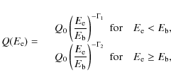
where Q0 is a normalization constant,
In this equation the parameter
|
(3) |
In this expression,
|
(4) |
where B is the magnetic field strength in Gauss. The lower
Our model introduced in this article is aimed at modeling the
nonthermal emission of the PWN close to the pulsar. In this region,
only a young population of leptons is expected. It is therefore
reasonable to neglect the time-dependence of the injection spectrum for
our model. Furthermore, we focus on the modeling of the X-ray spectrum
and the inverse Compton (IC) spectrum in the very high energy (VHE) ![]() -ray
regime. For this purpose, only the power-law component beyond the break
energy is relevant and we will thus assume a pure power law with
-ray
regime. For this purpose, only the power-law component beyond the break
energy is relevant and we will thus assume a pure power law with
![]() in the remainder of the paper. This implies that
in the remainder of the paper. This implies that ![]() is only a lower limit on the conversion efficiency, since we do not take the leptons with energies below
is only a lower limit on the conversion efficiency, since we do not take the leptons with energies below ![]() into account in our model.
into account in our model.
4.2 Propagation of the leptons in the PWN
In the downstream flow beyond the termination shock the particles lose energy, causing the shape of the lepton spectrum to change. In our model we use the approximation of a spherical symmetry. This implies that the propagation of the particles in the nebular flow of the PWN is strictly radial. Looking at the X-ray sky map of MSH 15-52 (see Fig. 1), a deviation from a spherical symmetry is apparent. However, compared to current models in which no spatial variation of the properties of the lepton population is taken into account, the radial approach should provide a good first estimate of the effects of spatial variation in the PWN.
Assuming that the magnetic field in the PWN is toroidal, Kennel & Coroniti (1984a) showed that the product of the flow velocity v, the distance from the pulsar r and the magnetic field strength B is a constant:
where the subscripted parameters denote the parameters at the shock. This is valid for a steady-state solution in the ideal magnetohydrodynamic limit. The post-shocked magnetic field strength is then given by (Kennel & Coroniti 1984a; Sefako & de Jager 2003)

|
(6) |
In this equation, and for the parameter optimization, we use
Since we assume the approximation of a radial outflow of the leptons in
the nebular flow, we can describe the bulk velocity of the leptons by a
profile depending only on ![]() and the distance to the pulsar, r. We adopt a profile of the form
and the distance to the pulsar, r. We adopt a profile of the form
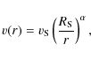
with an exponential index
The next step is to look at the change of the lepton spectrum as
the particles propagate away from the pulsar wind shock. The particles
lose energy due to adiabatic losses and synchrotron radiation in the
magnetic field of the PWN. The total energy loss of the particles is
given by (cf. de Jager & Harding 1992):
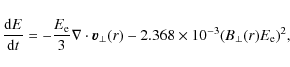
where the first part represents the adiabatic losses and the second part the energy losses due to synchrotron radiation.
4.3 Emission spectra
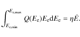
The parameters of the lepton population and the magnetic field are described for all locations in the PWN by Eqs. (5) to (8). With this information we are able to calculate the spectra of the synchrotron and inverse Compton radiation emitted by the leptons. For the calculation of the two emission processes, we use the standard equations by Blumenthal & Gould (1970).
We are now able to calculate the total emission for the lepton population at each point in the PWN. The emission from the model calculations is summed up to match the regions as observed in the XMM-Newton analysis (see Sect. 3). By comparing the measured synchrotron spectra with the calculated spectra we are able to constrain the free parameters of our model.
5 Parameter optimization
The optimization of the parameters of the model, as introduced in Sect. 4, was carried out by dividing the PWN into a number of shells. As discussed in the previous section, the values of v and B are known for every location in the PWN, thus enabling us to calculate the amount of energy lost by a particle during its propagation from the shock up to a specified shell. This, in turn, allows us to calculate the lepton spectrum that enters a shell, as well as the change in the lepton spectrum as it propagates through the shell. To calculate the corresponding nonthermal spectra, the initial lepton spectrum is used. This is sufficient, provided that the size of the shells is chosen small enough. The modified spectrum is then used as the injection spectrum for the following shell. For the first shell, the lepton spectrum is calculated by making use of Eq. (1), i.e. the lepton injection spectrum at the shock.
Since our modeling focuses only on the X-ray synchrotron component, we use a single power law, with
![]() ,
for the lepton injection spectrum. The index of the lepton spectrum is
derived from measurements of the photon spectrum close to the
termination shock with the Chandra
X-ray telescope, which yielded a photon index of around 1.5 (Y09).
Assuming that the lepton population emitting this spectrum has not
undergone any significant cooling, the spectral index of the lepton
spectrum is then equal to 2, which we adopt for our optimizations. G02
concluded that the spectral break between the comparatively flat radio
spectrum and the steeper synchrotron spectrum is just below the X-ray
band. Thus it is reasonable to assume
,
for the lepton injection spectrum. The index of the lepton spectrum is
derived from measurements of the photon spectrum close to the
termination shock with the Chandra
X-ray telescope, which yielded a photon index of around 1.5 (Y09).
Assuming that the lepton population emitting this spectrum has not
undergone any significant cooling, the spectral index of the lepton
spectrum is then equal to 2, which we adopt for our optimizations. G02
concluded that the spectral break between the comparatively flat radio
spectrum and the steeper synchrotron spectrum is just below the X-ray
band. Thus it is reasonable to assume
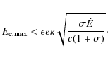
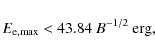
![]() to be of order 1 erg. Since only the logarithm of
to be of order 1 erg. Since only the logarithm of
![]() contributes to the normalization of the spectrum, a variation of
contributes to the normalization of the spectrum, a variation of
![]() does not change the spectral shape and has little effect on the total flux.
does not change the spectral shape and has little effect on the total flux.
The remaining free parameters of the model are then the shock radius ![]() ,
the bulk velocity of the leptons at the shock
,
the bulk velocity of the leptons at the shock ![]() ,
the index of the velocity profile
,
the index of the velocity profile ![]() ,
the conversion efficiency of spin-down luminosity into lepton energy
,
the conversion efficiency of spin-down luminosity into lepton energy ![]() and the parameter
and the parameter ![]() ,
which links the magnetization
,
which links the magnetization ![]() and the compression
and the compression ![]() of the shock. The parameters
of the shock. The parameters ![]() and
and ![]() are restricted by the observations of G02 and Y09, whereas the
other parameters are left unconstrained for the optimization. To
determine the optimum fit to the synchrotron spectra for the different
scenarios, we minimized the
are restricted by the observations of G02 and Y09, whereas the
other parameters are left unconstrained for the optimization. To
determine the optimum fit to the synchrotron spectra for the different
scenarios, we minimized the ![]() test statistic for the XMM-Newton data points and the calculated model flux points.
test statistic for the XMM-Newton data points and the calculated model flux points.
For PSR B1509-58, G02 and Y09 both estimated the termination shock radius using Chandra
data, but do not find consistent results. G02 favor a scenario in
which a feature at 0.5 pc corresponds to an internal structure in
the termination shock. They also estimated the ![]() value for several compact knots of emission less than 0.5 pc away
from the pulsar and concluded that the transition to a
particle-dominated wind should occur at a distance less than
0.1 pc from the pulsar. Y09 analyzed a considerably larger data
set of Chandra
observations and used image enhancement techniques to resolve the
detailed structure of the inner region around PSR B1509-58.
According to their results, the termination shock is located at a
distance of 9'' to the pulsar, which corresponds to a termination shock
radius of
value for several compact knots of emission less than 0.5 pc away
from the pulsar and concluded that the transition to a
particle-dominated wind should occur at a distance less than
0.1 pc from the pulsar. Y09 analyzed a considerably larger data
set of Chandra
observations and used image enhancement techniques to resolve the
detailed structure of the inner region around PSR B1509-58.
According to their results, the termination shock is located at a
distance of 9'' to the pulsar, which corresponds to a termination shock
radius of
![]() pc. For the magnetization parameter, Y09 derived a value of
pc. For the magnetization parameter, Y09 derived a value of
![]() ,
which is about a factor of 2 greater than the result obtained by G02.
,
which is about a factor of 2 greater than the result obtained by G02.
Based on the two analyses, we considered three scenarios with different values for ![]() for the optimization procedure of our model. In Scenario I we assume that the termination shock is unresolved in the Chandra
observations by G02 and Y09 and thus is at a distance closer than
0.1 pc from the pulsar. For Scenario II we assume a distance
of
for the optimization procedure of our model. In Scenario I we assume that the termination shock is unresolved in the Chandra
observations by G02 and Y09 and thus is at a distance closer than
0.1 pc from the pulsar. For Scenario II we assume a distance
of
![]() pc, while for Scenario III we adopt the value of
pc, while for Scenario III we adopt the value of
![]() pc, as stated by Y09.
pc, as stated by Y09.
G02 and Y09 both assume a shock velocity of
![]() .
The same value was also found for other PWN, e.g. the Crab Nebula (Kennel & Coroniti 1984a).
Furthermore, this shock velocity is in good agreement with the lower
limit that G02 determined from the energetics of the PWN. Therefore, we
also adopted this value for our calculations.
We do not constrain the remaining parameters
.
The same value was also found for other PWN, e.g. the Crab Nebula (Kennel & Coroniti 1984a).
Furthermore, this shock velocity is in good agreement with the lower
limit that G02 determined from the energetics of the PWN. Therefore, we
also adopted this value for our calculations.
We do not constrain the remaining parameters ![]() ,
,
![]() and
and ![]() ,
except for the straight-forward assumption that the conversion efficiency
,
except for the straight-forward assumption that the conversion efficiency ![]() should be in the interval
should be in the interval
![]() .
Table 4
gives an overview of the three scenarios and the constraints on the
parameters, which we used for the modeling described in the next
section.
.
Table 4
gives an overview of the three scenarios and the constraints on the
parameters, which we used for the modeling described in the next
section.
Table 4: Model parameters for the different scenarios as discussed in the text.
6 Results of the modeling
Using the model and the parameter constraints described in the
previous section, we calculated the optimum parameters for the three
scenarios defined in Sect. 5.
The results of the optimization show that the Scenarios II and III
(larger shock radius) yield a better fit to the data than
Scenario I (small shock radius). For Scenario I we do not
have a fixed value for ![]() .
We thus leave it as a free parameter for the simulations. The best fit for this scenario is obtained for a value of
.
We thus leave it as a free parameter for the simulations. The best fit for this scenario is obtained for a value of
![]() pc which is the upper limit for
pc which is the upper limit for ![]() (see Table 4).
However, even the best fit of Scenario I does not give a
satisfactory result. Due to the small shock radius, the synchrotron
cooling is very efficient and leads to a strong cutoff in the X-ray
spectra for the outer rings, which is not consistent with the observed
emission.
(see Table 4).
However, even the best fit of Scenario I does not give a
satisfactory result. Due to the small shock radius, the synchrotron
cooling is very efficient and leads to a strong cutoff in the X-ray
spectra for the outer rings, which is not consistent with the observed
emission.
![\begin{figure}
\par\includegraphics[width=9cm,clip]{14151fg05.eps}
\end{figure}](/articles/aa/full_html/2010/07/aa14151-10/img77.png)
|
Figure 5: Data and model spectra for the ring 1 and 6 regions for Scenario II. The shaded regions mark the error bands of the XMM-Newton measurement of ring 1 and 6. For ring 1 the error band is very narrow and thus hardly visible. |
| Open with DEXTER | |
![\begin{figure}
\par\includegraphics[width=9cm,clip]{14151fg06.eps}
\end{figure}](/articles/aa/full_html/2010/07/aa14151-10/img78.png)
|
Figure 6: Spectral indices of power-law fits to the XMM-Newton data of the different regions in the energy range of 0.5-9.0 keV. The model points shown are calculated for the best fit of Scenario II and use the same energy range for the fit. |
| Open with DEXTER | |
![\begin{figure}
\par\includegraphics[width=9cm,clip]{14151fg07.eps}
\end{figure}](/articles/aa/full_html/2010/07/aa14151-10/img79.png)
|
Figure 7: Variation of the surface brightness for the XMM-Newton data and the model in the energy range of 0.5-9.0 keV. The model points shown are calculated for the best fit of Scenario II. |
| Open with DEXTER | |
![\begin{figure}
\par\includegraphics[width=9cm,clip]{14151fg08.eps}
\end{figure}](/articles/aa/full_html/2010/07/aa14151-10/img80.png)
|
Figure 8: Data and model spectra for the ring 1 and 6 regions for Scenario III. The shaded regions mark the error bands of the XMM-Newton measurement of ring 1 and 6. For ring 1 the error band is very narrow and thus hardly visible. |
| Open with DEXTER | |
![\begin{figure}
\par\includegraphics[width=9cm,clip]{14151fg09.eps}
\end{figure}](/articles/aa/full_html/2010/07/aa14151-10/img81.png)
|
Figure 9: Spectral indices of power-law fits to the XMM-Newton data of the different regions in the energy range of 0.5-9.0 keV. The model points shown are calculated for the best fit of Scenario III and use the same energy range for the fit. |
| Open with DEXTER | |
![\begin{figure}
\par\includegraphics[width=9cm,clip]{14151fg10.eps}
\end{figure}](/articles/aa/full_html/2010/07/aa14151-10/img82.png)
|
Figure 10: Variation of the surface brightness for the XMM-Newton data and the model in the energy range of 0.5-9.0 keV. The model points shown are calculated for the best fit of Scenario III. |
| Open with DEXTER | |
![\begin{figure}
\par\includegraphics[width=9cm,clip]{14151fg11.eps}
\end{figure}](/articles/aa/full_html/2010/07/aa14151-10/img83.png)
|
Figure 11:
Spatial evolution of the magnetic field with distance from the pulsar.
The two solid lines denote the upper and lower range of values of the
magnetic field strength for Scenario II (based on the range for |
| Open with DEXTER | |
The results obtained for Scenarios II and III constrain the range
of the model parameters. Since the parameters are correlated, it is
only possible to state parameter ranges. For Scenario II we found
that the index of the velocity profile is in the range of
![]() .
The conversion efficiency is greater than 0.3 for this scenario and
.
The conversion efficiency is greater than 0.3 for this scenario and ![]() ranges between 0.3 and 1.3. The compression ratio
ranges between 0.3 and 1.3. The compression ratio ![]() varies between 1 and 3 for relativistic shocks. We can thus translate the range of
varies between 1 and 3 for relativistic shocks. We can thus translate the range of ![]() to the result that
to the result that
![]() ,
which is a factor of 2 more than the lower limit derived by G02. For Scenario III, we found the same range for
,
which is a factor of 2 more than the lower limit derived by G02. For Scenario III, we found the same range for ![]() and
and ![]() ,
but a narrower lower limit on the magnetization parameter,
,
but a narrower lower limit on the magnetization parameter,
![]() .
This is lower than the limit that Y09 found in their estimate based on
the equipartition assumption. In summary, we can state that our results
support a shock radius of the order of 0.2 - 0.5 pc. However, we are not
able to favor one scenario above the other. For the conversion
efficiency, we found a lower limit of
.
This is lower than the limit that Y09 found in their estimate based on
the equipartition assumption. In summary, we can state that our results
support a shock radius of the order of 0.2 - 0.5 pc. However, we are not
able to favor one scenario above the other. For the conversion
efficiency, we found a lower limit of
![]() for Scenario II and III. This agrees very well with the result of the time-dependent one-zone model by Zhang et al. (2008). The magnetic field estimates for MSH 15-52 range between 8
for Scenario II and III. This agrees very well with the result of the time-dependent one-zone model by Zhang et al. (2008). The magnetic field estimates for MSH 15-52 range between 8 ![]() G (G02) and 25
G (G02) and 25 ![]() G (Zhang et al. 2008). The spatial evolution of the magnetic field with distance for our model can be seen in Fig. 11. Our predictions for the magnetic field in the PWN agree with the estimates from the other authors.
The lower limit of
G (Zhang et al. 2008). The spatial evolution of the magnetic field with distance for our model can be seen in Fig. 11. Our predictions for the magnetic field in the PWN agree with the estimates from the other authors.
The lower limit of
![]() on the magnetization parameter agrees very well with the observational results obtained with the Chandra satellite by G02 and Y09, which both state a lower limit of the same value as we derive with our model.
on the magnetization parameter agrees very well with the observational results obtained with the Chandra satellite by G02 and Y09, which both state a lower limit of the same value as we derive with our model.
![\begin{figure}
\par\includegraphics[width=9cm,clip]{14151fg12.eps}
\end{figure}](/articles/aa/full_html/2010/07/aa14151-10/img89.png)
|
Figure 12:
Smoothed HESS excess map of the VHE |
| Open with DEXTER | |
![\begin{figure}
\par\includegraphics[width=9cm,clip]{14151fg13.eps}
\end{figure}](/articles/aa/full_html/2010/07/aa14151-10/img90.png)
|
Figure 13:
Spectral index of a power-law fit to the IC emission calculated in the
model with increasing distance from the pulsar. The fit range was from
300 GeV to 30 TeV. Plotted is the result of the model with
the best fit parameters for Scenario II for a conversion
efficiency of
|
| Open with DEXTER | |
7 Implications for the TeV  -ray emission
Based on the optimized parameters described in the previous section, we
calculated the IC emission for our model to compare it to the
observational TeV ![]() -ray data. MSH 15-52 is an extended source in VHE
-ray data. MSH 15-52 is an extended source in VHE ![]() -rays and was detected by the HESS experiment (Aharonian et al. 2005).
The emission in the VHE energy band extends beyond the central
part of the PWN that is considered in our model. Thus, we used the
published VHE excess events map to rescale the spectrum to the central
300 arcsec region around the pulsar. The excess map, smoothed with
a Gaussian with the size of the point spread function (
-rays and was detected by the HESS experiment (Aharonian et al. 2005).
The emission in the VHE energy band extends beyond the central
part of the PWN that is considered in our model. Thus, we used the
published VHE excess events map to rescale the spectrum to the central
300 arcsec region around the pulsar. The excess map, smoothed with
a Gaussian with the size of the point spread function (![]()
![]() ), is shown in Fig. 12.
The ratio of excess events between the two regions used in the HESS
publication and for our modeling is 3.42. The rescaled
normalization of the
), is shown in Fig. 12.
The ratio of excess events between the two regions used in the HESS
publication and for our modeling is 3.42. The rescaled
normalization of the
![]() -ray spectrum at 1 TeV is then
-ray spectrum at 1 TeV is then
![]() 10-12 TeV-1 cm-2 s-1,
where we rescale the errors with the same factor. Our rescaling assumes
that there is no significant spectral variation for the HESS spectrum,
i.e. the photon index of the measured index is equal to
10-12 TeV-1 cm-2 s-1,
where we rescale the errors with the same factor. Our rescaling assumes
that there is no significant spectral variation for the HESS spectrum,
i.e. the photon index of the measured index is equal to
![]() throughout the extraction region. Another important aspect to consider is the size of the HESS PSF. Since the extension of its
throughout the extraction region. Another important aspect to consider is the size of the HESS PSF. Since the extension of its ![]() containment radius is of the same order as our extraction region (
containment radius is of the same order as our extraction region (
![]() deg), we expect some contamination in our extraction region from the outer regions of the PWN. About
deg), we expect some contamination in our extraction region from the outer regions of the PWN. About ![]() of the emission from inside the PSF will fall outside of the region
defined by the rings 1 to 6. However, a similar amount from
the emission outside the PSF region will fall into the central PSF
region (i.e. ring 1 to 6). These effects will cancel to a
first order, although a systematic steepening in the spectrum is
expected if the TeV photon index also steepens with increasing radius,
as is predicted by our model. Figure 13
shows the spectral index for the IC emission with increasing distance
of the region from the pulsar, where it can be seen that the index
steepens by
of the emission from inside the PSF will fall outside of the region
defined by the rings 1 to 6. However, a similar amount from
the emission outside the PSF region will fall into the central PSF
region (i.e. ring 1 to 6). These effects will cancel to a
first order, although a systematic steepening in the spectrum is
expected if the TeV photon index also steepens with increasing radius,
as is predicted by our model. Figure 13
shows the spectral index for the IC emission with increasing distance
of the region from the pulsar, where it can be seen that the index
steepens by
![]() .
.
Figure 14 shows a plot of the spectral energy distribution (SED) of MSH 15-52 in the X-ray and TeV
![]() -ray
band. The presented experimental data in the X-ray band are the sum of
the emission of the shells from the XMM-Newton analysis (see Sect. 3).
For the TeV range, the rescaled HESS spectrum is shown. The model
SED was obtained with the best fit parameters of Scenario II (
-ray
band. The presented experimental data in the X-ray band are the sum of
the emission of the shells from the XMM-Newton analysis (see Sect. 3).
For the TeV range, the rescaled HESS spectrum is shown. The model
SED was obtained with the best fit parameters of Scenario II (![]() = 0.5 pc) for a conversion efficiency of
= 0.5 pc) for a conversion efficiency of
![]() .
For this set of parameters, the fitted spectral index to the IC
emission in the 0.3-30 TeV energy range is 1.8 and thus slightly
below the statistical and systematic errors of the measured HESS
spectrum. The normalization of the fit is 3.1
.
For this set of parameters, the fitted spectral index to the IC
emission in the 0.3-30 TeV energy range is 1.8 and thus slightly
below the statistical and systematic errors of the measured HESS
spectrum. The normalization of the fit is 3.1 ![]() 10-12 TeV-1 cm-2 s-1 and hence also below the
10-12 TeV-1 cm-2 s-1 and hence also below the ![]() errors of the measurement. The ratio of the predicted flux above
0.3 TeV for this set of parameters to the observed flux is 0.3.
errors of the measurement. The ratio of the predicted flux above
0.3 TeV for this set of parameters to the observed flux is 0.3.
The change in surface brightness of the IC emission is shown in Fig. 15. The flux was calculated in the energy interval of 0.3-30 TeV and for the same ring regions as used in the X-ray analysis. Unfortunately, with the angular resolution of the HESS experiment it is not possible to test the model against the data. Future Imaging Air Cherenkov Telescopes like the Cherenkov Telescope Array (CTA, Wagner et al. 2009) will have a resolution around one arcminute and will allow for a test of these predictions. Compared to the X-ray surface brightness, which drops by three orders of magnitude from ring 1 to ring 6, the drop in the surface brightness of the IC emission is considerably smaller. However, from looking at the VHE sky map (Fig. 12) one can see, that the emission must have a large component which is not described by our model. This might, for example, be due to an older population of electrons.
![\begin{figure}
\par\includegraphics[width=9cm,clip]{14151fg14.eps}
\end{figure}](/articles/aa/full_html/2010/07/aa14151-10/img100.png)
|
Figure 14:
Spectral energy distribution of MSH 15-52 from the extraction regions as marked in Fig. 12.
The XMM-Newton and the HESS data are marked as solid lines, the model
results for the best fit values of Scenario II with a conversion
efficiency of
|
| Open with DEXTER | |
![\begin{figure}
\par\includegraphics[width=9cm,clip]{14151fg15.eps}
\end{figure}](/articles/aa/full_html/2010/07/aa14151-10/img101.png)
|
Figure 15:
Surface brightness of the IC emission with increasing distance from the
pulsar. The surface brightness was calculated for a power-law fit to
the data in an energy range of 300 GeV to 30 TeV. Plotted is
the emission from the model calculations with the best fit parameters
for Scenario II for a conversion efficiency of
|
| Open with DEXTER | |
8 Conclusion
We analyzed XMM-Newton data of the SNR MSH 15-52 to derive the spatially resolved spectral parameters of the inner region of the source. For this analysis we extracted spectra from six annuli centered on PSR B1509-58. A steepening of the X-ray spectrum with increasing distance from the pulsar is observed. The surface brightness in the XMM-Newton range drops by three orders of magnitude from the inner region close to PSR B1509-58 up to the last ring used in our analysis (at a distance of 300 arcsec from the pulsar). The spectra of all rings are fitted well with power laws.
We then introduced a numerical model to describe the spatial evolution of the lepton population and the magnetic field within the PWN. Our model is based on the parameters of the termination shock. We fitted the calculated model spectra to the XMM-Newton data to constrain the parameters of our model. The results of our optimizations suggest a termination shock in the range of 0.225 to 0.5 pc (Scenarios II and III in this work), which are the values derived from different analyses by G02 and Y09. However, the results of the optimizations of our model do not favor one scenario over the other. For the magnetization parameter, we arrive at a lower limit of 0.005, while our lower limit on the conversion efficiency is 0.3.
Using the model parameters obtained from the fit to the X-ray
data, we calculated the IC emission from the lepton population in the
PWN. We rescaled the published HESS data to compare the total IC
emission from our model with the observed emission. The results show
that our model reproduces the right order of magnitude for the observed
IC flux, but differs slightly in the spectral shape of the emission.
However, we did not take into account contamination effects for the VHE
photons due to the PSF. A steeper photon index outside the region used
for our model would lead to a systematically steeper spectrum inside
the region due to PSF spillover effects. This effect was not taken into
account in Fig. 14.
Additionally, we also calculated the spectral index and the surface
brightness with increasing distance of the regions from the pulsar,
which may be tested with future VHE ![]() -ray instruments like the CTA observatory.
-ray instruments like the CTA observatory.
The total energy that is emitted by the leptons in the inner region of
the PWN via synchrotron and IC emission in our model can be obtained by
integrating over the SED (see Fig. 14). The integrated emission of
![]() amounts to roughly
amounts to roughly ![]() of the current spin-down luminosity of PSR B1509-58. However, when
making this comparison one has to be aware that the integrated emission
comes from a population of leptons with different lifetimes and cannot
be directly linked to the current spin-down luminosity. Furthermore,
there is also significant emission at X-ray and TeV energies outside
the central
of the current spin-down luminosity of PSR B1509-58. However, when
making this comparison one has to be aware that the integrated emission
comes from a population of leptons with different lifetimes and cannot
be directly linked to the current spin-down luminosity. Furthermore,
there is also significant emission at X-ray and TeV energies outside
the central
![]() region considered in our modeling approach, which increases the
percentage of lepton energy converted to radiation (see Figs. 1 and 12).
region considered in our modeling approach, which increases the
percentage of lepton energy converted to radiation (see Figs. 1 and 12).
In summary, we show that our radially symmetric model of the PWN MSH 15-52
readily describes the nonthermal emissionseen in the X-ray band.
Despite the simplifying assumptions of our model, the change in
spectral index and surface brightness can be reproduced. The model is
also able to predict the flux level of the observed emission in VHE ![]() -rays,
however, the exact shape of the spectrum is not reproduced. For the
future, an application of the model introduced in this paper to other
PWN should be interesting to obtain a broader view on the underlying
physics in PWN.
-rays,
however, the exact shape of the spectrum is not reproduced. For the
future, an application of the model introduced in this paper to other
PWN should be interesting to obtain a broader view on the underlying
physics in PWN.
We would like to thank the anonymous referee for the constructive comments. They helped to improve the article significantly.
References
- Aharonian, F., Akhperjanian, A. G., Aye, K.-M., et al. 2005, A&A, 435, L17 [NASA ADS] [CrossRef] [EDP Sciences] [Google Scholar]
- Arnaud, K. A. 1996, in Astronomical Data Analysis Software and Systems V, ed. G. H. Jacoby, & J. Barnes, ASP Conf. Ser., 101, 17 [Google Scholar]
- Blumenthal, G. R., & Gould, R. J. 1970, Rev. Mod. Phys., 42, 237 [NASA ADS] [CrossRef] [Google Scholar]
- de Jager, O. C., & Djannati-Ataï, A. 2009, Neutron Stars and Pulsars, ed. W. Becker, ASSL, 357, 451 (Springer) [Google Scholar]
- de Jager, O. C., & Harding, A. K. 1992, ApJ, 396, 161 [NASA ADS] [CrossRef] [Google Scholar]
- Forot, M., Hermsen, W., Renaud, M., et al. 2006, ApJ, 651, L45 [NASA ADS] [CrossRef] [Google Scholar]
- Gaensler, B. M., Arons, J., Kaspi, V. M., et al. 2002, ApJ, 569, 878 [CrossRef] [Google Scholar]
- Gaensler, B. M., Brazier, K. T. S., Manchester, R. N., Johnston, S., & Green, A. J. 1999, MNRAS, 305, 724 [NASA ADS] [CrossRef] [Google Scholar]
- Gaensler, B. M., & Slane, P. O. 2006, ARA&A, 44, 17 [NASA ADS] [CrossRef] [Google Scholar]
- Jansen, F., Lumb, D., Altieri, B., et al. 2001, A&A, 365, L1 [NASA ADS] [CrossRef] [EDP Sciences] [Google Scholar]
- Kaspi, V. M., Manchester, R. N., Siegman, B., Johnston, S., & Lyne, A. G. 1994, ApJ, 422, L83 [NASA ADS] [CrossRef] [Google Scholar]
- Kennel, C. F., & Coroniti, F. V. 1984a, ApJ, 283, 694 [NASA ADS] [CrossRef] [Google Scholar]
- Kennel, C. F., & Coroniti, F. V. 1984b, ApJ, 283, 710 [NASA ADS] [CrossRef] [Google Scholar]
- Mills, B. Y., Slee, O. B., & Hill, E. R. 1961, Aust. J. Phys., 14, 497 [NASA ADS] [CrossRef] [Google Scholar]
- Mineo, T., Cusumano, G., Maccarone, M. C., et al. 2001, A&A, 380, 695 [NASA ADS] [CrossRef] [EDP Sciences] [Google Scholar]
- Reynolds, S. P., & Chevalier, R. A. 1984, ApJ, 278, 630 [NASA ADS] [CrossRef] [Google Scholar]
- Sefako, R. R., & de Jager, O. C. 2003, ApJ, 593, 1013 [NASA ADS] [CrossRef] [Google Scholar]
- Seward, F. D., & Harnden, Jr., F. R. 1982, ApJ, 256, L45 [NASA ADS] [CrossRef] [Google Scholar]
- Strüder, L., Briel, U., Dennerl, K., et al. 2001, A&A, 365, L18 [NASA ADS] [CrossRef] [EDP Sciences] [Google Scholar]
- Tamura, K., Kawai, N., Yoshida, A., & Brinkmann, W. 1996, PASJ, 48, L33 [NASA ADS] [CrossRef] [Google Scholar]
- Trussoni, E., Massaglia, S., Caucino, S., Brinkmann, W., & Aschenbach, B. 1996, A&A, 306, 581 [NASA ADS] [Google Scholar]
- Turner, M. J. L., Abbey, A., Arnaud, M., et al. 2001, A&A, 365, L27 [NASA ADS] [CrossRef] [EDP Sciences] [Google Scholar]
- Venter, C., & de Jager, O. C. 2007, in Proceedings of the 363, WE-Heraeus Seminar on Neutron Stars and Pulsars 40 years after the discovery, MPE-Report 291, ISSN 0178-0719 (Garching bei München, Germany: Max Planck Institut für extraterrestrische Physik), ed. W. Becker, & H. H. Huang, 40 [Google Scholar]
- Wagner, R. M., Lindfors, E. J., Sillanpää, A., et al. 2009 [arXiv:0912.3742] [Google Scholar]
- Wilms, J., Allen, A., & McCray, R. 2000, ApJ, 542, 914 [NASA ADS] [CrossRef] [Google Scholar]
- Yatsu, Y., Kawai, N., Shibata, S., & Brinkmann, W. 2009, PASJ, 61, 129 [NASA ADS] [Google Scholar]
- Zhang, L., Chen, S. B., & Fang, J. 2008, ApJ, 676, 1210 [NASA ADS] [CrossRef] [Google Scholar]
All Tables
Table 1: Details of the XMM-Newton EPIC PN observations on MSH 15-52.
Table 2: Extraction regions for the XMM-Newton spectral analysis of the source.
Table 3: Results obtained by fitting a power-law spectrum to the XMM-Newton data of MSH 15-52.
Table 4: Model parameters for the different scenarios as discussed in the text.
All Figures
|
|
Figure 1: XMM-Newton count map of MSH 15-52 showing the six extraction regions (numbered and marked by white lines) and the exclusion region (black dashed line) used for the spectral analysis. The six extraction regions are centered on the position of the pulsar PSR B1509-58. The exclusion region was chosen to encompass the thermal emission from the H II region RCW 89. |
| Open with DEXTER | |
| In the text | |
|
|
Figure 2: Spectrum and power-law fit for the first extraction region (ring 1). Two observations were used for the analysis of this region (cf. Table 2). The resulting fit parameters are listed in Table 3. |
| Open with DEXTER | |
| In the text | |
|
|
Figure 3: Spectral index of the power-law fit to the XMM-Newton data of the different regions versus the mean distance of the extraction regions to the pulsar. A steepening of the spectrum is observed with increasing distance. |
| Open with DEXTER | |
| In the text | |
|
|
Figure 4: Surface brightness of the X-ray emission of the PWN in the 0.5-9.0 keV band as a function of the distance to the pulsar. |
| Open with DEXTER | |
| In the text | |
|
|
Figure 5: Data and model spectra for the ring 1 and 6 regions for Scenario II. The shaded regions mark the error bands of the XMM-Newton measurement of ring 1 and 6. For ring 1 the error band is very narrow and thus hardly visible. |
| Open with DEXTER | |
| In the text | |
|
|
Figure 6: Spectral indices of power-law fits to the XMM-Newton data of the different regions in the energy range of 0.5-9.0 keV. The model points shown are calculated for the best fit of Scenario II and use the same energy range for the fit. |
| Open with DEXTER | |
| In the text | |
|
|
Figure 7: Variation of the surface brightness for the XMM-Newton data and the model in the energy range of 0.5-9.0 keV. The model points shown are calculated for the best fit of Scenario II. |
| Open with DEXTER | |
| In the text | |
|
|
Figure 8: Data and model spectra for the ring 1 and 6 regions for Scenario III. The shaded regions mark the error bands of the XMM-Newton measurement of ring 1 and 6. For ring 1 the error band is very narrow and thus hardly visible. |
| Open with DEXTER | |
| In the text | |
|
|
Figure 9: Spectral indices of power-law fits to the XMM-Newton data of the different regions in the energy range of 0.5-9.0 keV. The model points shown are calculated for the best fit of Scenario III and use the same energy range for the fit. |
| Open with DEXTER | |
| In the text | |
|
|
Figure 10: Variation of the surface brightness for the XMM-Newton data and the model in the energy range of 0.5-9.0 keV. The model points shown are calculated for the best fit of Scenario III. |
| Open with DEXTER | |
| In the text | |
|
|
Figure 11:
Spatial evolution of the magnetic field with distance from the pulsar.
The two solid lines denote the upper and lower range of values of the
magnetic field strength for Scenario II (based on the range for |
| Open with DEXTER | |
| In the text | |
|
|
Figure 12:
Smoothed HESS excess map of the VHE |
| Open with DEXTER | |
| In the text | |
|
|
Figure 13:
Spectral index of a power-law fit to the IC emission calculated in the
model with increasing distance from the pulsar. The fit range was from
300 GeV to 30 TeV. Plotted is the result of the model with
the best fit parameters for Scenario II for a conversion
efficiency of
|
| Open with DEXTER | |
| In the text | |
|
|
Figure 14:
Spectral energy distribution of MSH 15-52 from the extraction regions as marked in Fig. 12.
The XMM-Newton and the HESS data are marked as solid lines, the model
results for the best fit values of Scenario II with a conversion
efficiency of
|
| Open with DEXTER | |
| In the text | |
|
|
Figure 15:
Surface brightness of the IC emission with increasing distance from the
pulsar. The surface brightness was calculated for a power-law fit to
the data in an energy range of 300 GeV to 30 TeV. Plotted is
the emission from the model calculations with the best fit parameters
for Scenario II for a conversion efficiency of
|
| Open with DEXTER | |
| In the text | |
Copyright ESO 2010
Current usage metrics show cumulative count of Article Views (full-text article views including HTML views, PDF and ePub downloads, according to the available data) and Abstracts Views on Vision4Press platform.
Data correspond to usage on the plateform after 2015. The current usage metrics is available 48-96 hours after online publication and is updated daily on week days.
Initial download of the metrics may take a while.