| Issue |
A&A
Volume 515, June 2010
|
|
|---|---|---|
| Article Number | A96 | |
| Number of page(s) | 6 | |
| Section | The Sun | |
| DOI | https://doi.org/10.1051/0004-6361/200913829 | |
| Published online | 15 June 2010 | |
Anisotropic viscous dissipation in transient reconnecting plasmas
I. J. D. Craig
Department of Mathematics, University of Waikato, P. B. 3105, Hamilton, New Zealand
Received 9 December 2009 / Accepted 8 March 2010
Abstract
Aims. We examine the global energy losses associated with reconnecting coronal plasmas.
Methods. Using planar magnetic reconnection simulations we
compute resistive and bulk viscous losses in transient coronal plasmas.
Resistive scalings are computed for the case of incompressible
reconnection powered by large scale vortical flows. These results are
contrasted with an example of magnetic merging driven by the
coalescence instability.
Results. We demonstrate that the large scale advective flows,
required to sustain resistive current sheets, may be associated with
viscous losses approaching flare-like rates of 1029 erg s-1.
More generally, bulk viscous dissipation appears likely to dominate
resistive dissipation for a wide variety of magnetic merging models. We
emphasize that these results have potentially important implications
for understanding the flare energy budget.
Key words: magnetohydrodynamics (MHD) - Sun: flares - magnetic fields
1 Introduction
Magnetic reconnection is recognized as a key process in the evolution of coronal plasmas. Since reconnection is the only mechanism that can alter the magnetic field topology, it is thought crucial in a variety of applications, for instance, in the explosive release of the solar flare and in the theory of magnetic coronal heating (Priest & Forbes 2000). A recurring difficulty however, is the slow rate of the magnetic energy release due to the weak coronal resistivity. Unless this rate is enhanced in some manner, say by the inclusion of Hall effects (Knoll & Chacon 2006), or by the adoption of a turbulent resistivity (Litvinenko & Craig 2000), reconnection models are unlikely to meet the explosive energy release requirements of the solar flare.
Motivated largely by the energy release problem, there has been a concerted theoretical effort to incorporate extra physical ingredients into magnetic merging models. One promising approach is the adoption of a generalized Ohms law to account for non-collisional effects (Birn et al. 2001). It has been claimed for instance that Hall effects can speed up the reconnection rate independently of the size of the system (Cassak et al. 2006), a claim contested on the basis of kinematic reconnection simulations (Daughton et al. 2006) and X-point collapse merging (Craig & Litvinenko 2008). More recently, studies of 3D stochastic merging have suggested a ``fast'' regime in which the reconnection rate is effectively independent of the plasma resistivity (Kowal et al. 2009).
A further possibility is to account for the effects of viscosity
in the magnetic merging model.
Observational support for the presence viscous effects can be inferred
from studies of impulsive hard X-ray bursts (McKenzie &
Hudson 1999; Asai et al. 2004) which indicate that reconnective outflows
may be considerably slower than the Alfvénic exhausts predicted by
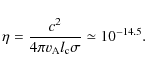
typical merging solutions. More theoretically, as emphasised by
Hollweg (1985, 1986), since the dimensionless
viscosity coefficient easily exceeds the normalized
resistivity - an inverse Lundquist number of order
![]() - viscous processes are likely to be important
in a wide variety of coronal processes. Yet although
the classical shear viscosity is routinely employed in
reconnection simulations, it often assumes a passive role, that of
simply stabilizing numerical
computations. In reality, shear viscous effects are likely to be
strongly suppressed in magnetically stratified plasmas such as the
solar corona: a more accurate treatment requires an anisotropic
bulk viscosity (Hollweg 1986).
- viscous processes are likely to be important
in a wide variety of coronal processes. Yet although
the classical shear viscosity is routinely employed in
reconnection simulations, it often assumes a passive role, that of
simply stabilizing numerical
computations. In reality, shear viscous effects are likely to be
strongly suppressed in magnetically stratified plasmas such as the
solar corona: a more accurate treatment requires an anisotropic
bulk viscosity (Hollweg 1986).
The purpose of the present study is to assess the role of viscous damping on transient magnetic reconnection solutions. This work extends recent analytic studies that focus on steady incompressible reconnection within ``open'' two and three dimensional geometries (Litvinenko 2005; Craig & Litvinenko 2009). By ``open'' we mean that energy dissipated within the reconnection region is continually replenished by energy fluxes through inflow boundary surfaces. In this type of flow-driven merging, bulk viscous losses are found to scale independently of the merging rate which is controlled essentially by the plasma resistivity. What is not clear is whether this property extends to more general physical situations or whether it appears as an artifact of the restricted analytic treatment.
In the present study we consider transient, incompressible reconnection within a ``closed'' magnetic geometry. The problem is formulated in Sect. 2 where we discuss appropriate forms for the bulk viscous tensor. Our central results, presented in Sect. 3, are obtained in a doubly periodic, planar configuration, and describe reconnection driven by large scale advective motions. These simulations are similar to those performed previously (e.g. Heerikhuisen et al. 2000) but differ by the inclusion an anisotropic bulk viscosity. To complement this analysis, Sect. 4 presents an example of ``magnetically driven'' visco-resistive reconnection: in this case the merging develops self-consistently from a loss of magnetic equilibrium. In Sect. 5 we summarize our findings.
2 The visco-resistive system
2.1 Governing MHD equations
The equations to be resolved are the MHD momentum and
induction equations for the magnetic and velocity fields. These
are scaled with respect to typical solar
coronal values for field strength
![]() ,
size scale
,
size scale
![]() and number density
and number density
![]() .
Times are measured in units of
.
Times are measured in units of
![]() where
where
![]() is the
Alfvén speed. The global energy loss rate has the units
is the
Alfvén speed. The global energy loss rate has the units
![]() .
.
We are interested in the evolution of the ![]() and
and ![]() fields in the presence of small viscous and
resistive damping coefficients. Since we consider planar,
incompressible plasmas, the constraint equations
fields in the presence of small viscous and
resistive damping coefficients. Since we consider planar,
incompressible plasmas, the constraint equations
![]() can be satisfied by adopting
the flux function and stream function representations
can be satisfied by adopting
the flux function and stream function representations
Introducing the Poisson bracket notation typified by
![\begin{displaymath}[\psi, \phi]= \partial_x \psi \partial_y \phi - \partial_y \psi
\partial_x \phi,
\end{displaymath}](/articles/aa/full_html/2010/07/aa13829-09/img28.png)
the momentum and induction equations take the dimensionless forms
![\begin{displaymath}\partial_t (\nabla^2 \phi) + [\nabla^2 \phi, \phi] =
[\nabla^2\psi, \psi] + G,
\end{displaymath}](/articles/aa/full_html/2010/07/aa13829-09/img29.png)
![\begin{displaymath}\partial_t \psi + [\psi, \phi] =
\eta \nabla^2 \psi.
\end{displaymath}](/articles/aa/full_html/2010/07/aa13829-09/img30.png)
Here
| (5) |
where
2.2 Resistive and viscous dissipation
Energy losses from the
source volume are controlled by two small parameters,
the dimensionless resistivity ![]() and the
dimensionless plasma viscosity
and the
dimensionless plasma viscosity ![]() .
For
a collisional plasma of temperature T = 106 K with conductivity
.
For
a collisional plasma of temperature T = 106 K with conductivity
![]() (Spitzer 1962),
(Spitzer 1962), ![]() is an inverse
Lundquist number of magnitude
is an inverse
Lundquist number of magnitude
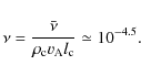
This number is considerably smaller than the Reynolds number associated with the viscous losses. For a plasma of mass density
Since
We conclude that the classical tensor ![]() for
the shear viscosity namely,
for
the shear viscosity namely,
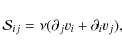
is generally inappropriate for magnetic coronal plasmas. More suitable is the strong field, bulk viscosity tensor (Braginskii 1965):
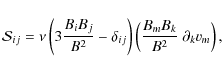
where summation over repeated suffixes is assumed. Note that a necessary condition for bulk viscous dissipation is that velocity gradients along the field lines be non-vanishing.
One minor complication is that the Braginskii tensor (9) cannot by extrapolated down to arbitrarily weak fields, for instance, those associated with magnetic nulls. In practice therefore we adopt the so called ``Liley form'' for the viscous tensor (Hosking & Marinoff 1973). This form, although not critical for the present applications, recovers expression (9) in strong field regions but also includes the weak field (shear viscosity) limit (8) that may apply sufficiently close to a magnetic null.
2.3 Global energy losses
In what follows we model reconnection within
a closed, periodic geometry (
![]() ). Of central
interest is a comparison of the Ohmic dissipation rate
). Of central
interest is a comparison of the Ohmic dissipation rate
where

Since it is not feasible to model the system for collisional resistivities approaching
3 Flow driven reconnection
3.1 The model
In this section we employ a doubly periodic code to model
transient reconnection (e.g. Watson
et al. 2007). An initial velocity field of the form
where
defines straight field lines, antiparallel about x = 0. These field lines rapidly distort as they are driven together by the flow (
![\begin{figure}
\par\includegraphics[width=9cm,clip]{13829fig1.eps}
\end{figure}](/articles/aa/full_html/2010/07/aa13829-09/img58.png)
|
Figure 1:
Time plot of the global Ohmic losses and bulk viscous dissipation.
The Ohmic losses
reflect the build up and localization of the current sheet. The
peak current density in the sheet J0 (divided by one
hundred for plotting purposes) is also shown. The plot is based on the
parameters
|
| Open with DEXTER | |
We shall not emphasize the phenomenology of the reconnection (see
Heerikhuisen et al. 2000; or Watson et al. 2007)
beyond noting that transient merging solutions produced
by strong cellular flows, and
analysed quantitatively at the time of maximum sheet development, are
known to provide an excellent ``snapshot'' of formally exact,
analytic merging solutions (Craig & Henton 1995). Figure 1 shows
the build up of the
current layer and the evolution of global losses up to the time of
maximum current density for the parameters
![]() and
b0 = 0.14. In this case, the resistivity is
large enough for the Ohmic dissipation rate
to increase to a level that exceeds the bulk viscous losses.
What is not so clear is whether this dominance can be maintained as the
resistivity is systematically reduced.
and
b0 = 0.14. In this case, the resistivity is
large enough for the Ohmic dissipation rate
to increase to a level that exceeds the bulk viscous losses.
What is not so clear is whether this dominance can be maintained as the
resistivity is systematically reduced.
Figure 2 shows field line contours at the end of the build up phase
(
![]() )
while Fig. 3 shows the corresponding current
density surface. Evidently a well defined, quasi
one-dimensional current layer has developed over the origin.
Note that identical reconnection sites are periodically
reproduced at each corner of the computational mesh.
)
while Fig. 3 shows the corresponding current
density surface. Evidently a well defined, quasi
one-dimensional current layer has developed over the origin.
Note that identical reconnection sites are periodically
reproduced at each corner of the computational mesh.
![\begin{figure}
\par\includegraphics[width=9cm,clip]{13829fig2.eps}
\end{figure}](/articles/aa/full_html/2010/07/aa13829-09/img59.png)
|
Figure 2:
Field line plot taken at the time of maximum current
density,
|
| Open with DEXTER | |
![\begin{figure}
\par\includegraphics[width=9cm,clip]{13829fig3.eps}
\end{figure}](/articles/aa/full_html/2010/07/aa13829-09/img60.png)
|
Figure 3:
Surface plot of the current density at the time of peak current
(
|
| Open with DEXTER | |
A surface plot of the vorticity of the flow is shown in Fig. 4. Regions of strong vorticity correspond quite closely to regions of high current density. Were the shear viscosity not suppressed by the magnetic field, we would expect strong viscous damping in these regions. The surface plot of bulk viscous dissipation shown in Fig. 5 indicates that significant damping can occur even when the vorticity is weak. Therefore, the identification of regions of strong viscous damping with regions of strong Ohmic heating is weakened in the case of bulk viscous losses.
![\begin{figure}
\par\includegraphics[width=9cm,clip]{13829fig4.eps}
\end{figure}](/articles/aa/full_html/2010/07/aa13829-09/img61.png)
|
Figure 4:
Surface plot of the vorticity at
|
| Open with DEXTER | |
![\begin{figure}
\includegraphics[width=9cm,clip]{13829fig5.eps}
\end{figure}](/articles/aa/full_html/2010/07/aa13829-09/img63.png)
|
Figure 5:
Surface plot of the volumetric bulk viscous dissipation
|
| Open with DEXTER | |
3.2 Resistive scalings
We now return to the problem of deducing resistive scalings for the
Ohmic and viscous losses. Note that it is not sufficient to simply
reduce ![]() while maintaining the intensity b0 of the
advected field. This is because, if the flux pile-up field
is allowed to build up too strongly, magnetic back pressures
develop that stall the flow
and arrest the development of the current layer. The
merging rate is then compromised by the break down of the large scale
vortical flows that drive the reconnection.
To maintain near-optimum Ohmic dissipation rates, b0 should be
adjusted to ensure that the current
sheet pressure at full development is comparable to the
dynamic pressure of the driving flow. Analytic arguments
suggest that taking
while maintaining the intensity b0 of the
advected field. This is because, if the flux pile-up field
is allowed to build up too strongly, magnetic back pressures
develop that stall the flow
and arrest the development of the current layer. The
merging rate is then compromised by the break down of the large scale
vortical flows that drive the reconnection.
To maintain near-optimum Ohmic dissipation rates, b0 should be
adjusted to ensure that the current
sheet pressure at full development is comparable to the
dynamic pressure of the driving flow. Analytic arguments
suggest that taking
![]() should provide a
practical guide for ensuring that the
peak magnetic field reflects the strength of the flow. With the peak
field normalized to the flow amplitude in this manner, the
current density builds up as
should provide a
practical guide for ensuring that the
peak magnetic field reflects the strength of the flow. With the peak
field normalized to the flow amplitude in this manner, the
current density builds up as
![]() (consistent with
traditional Sweet-Parker merging). It follows
that adequate resolution of the current layer requires grid sizes that
scale as
(consistent with
traditional Sweet-Parker merging). It follows
that adequate resolution of the current layer requires grid sizes that
scale as
![]() ,
corresponding to several hundred mesh points for
the lower resistivities
,
corresponding to several hundred mesh points for
the lower resistivities
![]() .
.
![\begin{figure}
\par\includegraphics[width=9cm,clip]{13829fig6.eps}
\end{figure}](/articles/aa/full_html/2010/07/aa13829-09/img68.png)
|
Figure 6:
Scaling with resistivity of the bulk viscous losses and the peak Ohmic
dissipation rate. The dashed reference line indicates an
|
| Open with DEXTER | |
Figure 6 shows resistive scalings obtained over the range
![]() for the parameters
for the parameters
![]() with
with
![]() .
The
systematic decline of the Ohmic losses with reductions in
.
The
systematic decline of the Ohmic losses with reductions in ![]() contrasts with the very weak dependency of the bulk viscous losses.
The fact that the Ohmic rate declines slightly faster than the
analytic
contrasts with the very weak dependency of the bulk viscous losses.
The fact that the Ohmic rate declines slightly faster than the
analytic
![]() expectation is
probably due to the decay of the global flow field. But although the peak
reconnecting field is always of order unity (commensurate with the
flow amplitude), we see that viscous damping starts
to dominate the Ohmic losses for
expectation is
probably due to the decay of the global flow field. But although the peak
reconnecting field is always of order unity (commensurate with the
flow amplitude), we see that viscous damping starts
to dominate the Ohmic losses for
![]() .
As expected
this dominance is found to increase with further reductions
in resistivity.
.
As expected
this dominance is found to increase with further reductions
in resistivity.
3.3 Summary
The present results suggest that viscous energy release could easily dominate resistive losses in typical coronal plasmas. For the flow driven reconnection model considered here, the viscous damping rate is insensitive to plasma resistivity.
To estimate the global viscous losses
we can multiply the dimensionless rate
![]() from Fig. 6
by the dimensional factor
from Fig. 6
by the dimensional factor
![]() ,
based on the typical coronal parameters of
Sect. 2.1. This suggests that flare-like damping rates exceeding 1029 erg s -1 could be achievable in practice. The
assumption of stronger driving flows
,
based on the typical coronal parameters of
Sect. 2.1. This suggests that flare-like damping rates exceeding 1029 erg s -1 could be achievable in practice. The
assumption of stronger driving flows
![]() could increase this rate
still further.
could increase this rate
still further.
Finally we should mention that the present results are unlikely to depend critically on the orientation of the initial disturbance field. This follows from the fact that axial field components, unlike the planar field (13), are not amplified by the flow as they are swept towards the reconnection region.
4 Merging driven by the coalescence instability
4.1 Introduction
One limitation of the previous reconnection model is the a priori assumption of a large scale vortical flow to drive the merging. It is not clear for instance how these results apply to magnetic merging driven say, by an initial magnetic imbalance or MHD instability. With this in mind we now consider an example of bulk viscous damping based on reconnection driven by the coalescence instability. Our aim is to illustrate how fluid motions, developing as part of the reconnection process, can lead to strong bulk viscous damping.
4.2 The coalescence simulation
The coalescence instability provides a self consistent, two-dimensional model for magnetic reconnection within a closed semi-periodic geometry (e.g Prichett & Wu 1979; Rickard & Craig 1993). The initial configuration comprises a periodic chain of magnetic islands. These slowly merge together in pairs, forming well-defined current sheets at which reconnection occurs.
The initial magnetic field is derived from the flux function
under the assumption of perfectly conducting walls at
defines the initial current density magnitude. However, provided the resistivity is not too large (say
![\begin{figure}
\par\includegraphics[width=9cm,clip]{13829fig7.eps}
\end{figure}](/articles/aa/full_html/2010/07/aa13829-09/img80.png)
|
Figure 7:
The flux function |
| Open with DEXTER | |
![\begin{figure}
\par\includegraphics[width=9cm,clip]{13829fig8.eps}
\end{figure}](/articles/aa/full_html/2010/07/aa13829-09/img81.png)
|
Figure 8:
The stream function |
| Open with DEXTER | |
Figures 7 and 8 show the stream and flux functions at the time of peak
current density for the parameters
![]() .
Although the bulk of the total
energy remains in the magnetic field - and it is the magnetic pressure
in the outer field that ultimately drives the merging - the
dynamic pressure of the flow develops to a level where it is
comparable to the magnetic pressure, especially in those regions of strong velocity gradient
close to the reconnection sites. The flow pattern is clearly dominated by two distinct,
clockwise rotating, cellular flows; one is centered on the
magnetic island, the other extends further into the outer magnetic field.
.
Although the bulk of the total
energy remains in the magnetic field - and it is the magnetic pressure
in the outer field that ultimately drives the merging - the
dynamic pressure of the flow develops to a level where it is
comparable to the magnetic pressure, especially in those regions of strong velocity gradient
close to the reconnection sites. The flow pattern is clearly dominated by two distinct,
clockwise rotating, cellular flows; one is centered on the
magnetic island, the other extends further into the outer magnetic field.
![\begin{figure}
\par\includegraphics[width=9cm,clip]{13829fig9.eps}
\end{figure}](/articles/aa/full_html/2010/07/aa13829-09/img82.png)
|
Figure 9:
Development of the Ohmic ( |
| Open with DEXTER | |
The resistivity in the present example has been chosen so that the
peak Ohmic and viscous dissipation rates remain comparable. More
specifically, Fig. 9 shows that the bulk viscous dissipation,
although entirely negligible for the first four or five Alfvén
times, is just starting to dominate the global losses by the
time that the peak current density is achieved. The viscous build up
accords with the dimensional estimate
![]() where vm is the peak speed of the flow.
where vm is the peak speed of the flow.
![\begin{figure}
\par\includegraphics[width=9cm,clip]{13829fig10.eps}
\end{figure}](/articles/aa/full_html/2010/07/aa13829-09/img85.png)
|
Figure 10:
Ohmic ( |
| Open with DEXTER | |
Figure 10 presents a sequence of exploratory runs that show
the effect of varying the resistivity
![]() while keeping all other parameters fixed in the simulation (
while keeping all other parameters fixed in the simulation (
![]() ). The dissipation rates are again evaluated
at the time of peak current density, but, unlike the results of Fig. 6,
no
attempt has been made to obtain ``saturated'' scalings by restricting
the strength of the field washed into the reconnection
region. The fact that the Ohmic losses are maintained against
reductions
in resistivity suggests that these results apply to a pre-saturation
regime in which ``fast'' reconnection is achieved by the continual
build-up of the field at the onset of the current layer.
Evidently the strengthening viscous losses at the smaller resistivities
are due to the increasing flow amplitude and alignment to the magnetic
field. The implication, physically, is that the global viscous losses
are likely to be significant even in the ``fast'' reconnection regime
prior to saturation.
). The dissipation rates are again evaluated
at the time of peak current density, but, unlike the results of Fig. 6,
no
attempt has been made to obtain ``saturated'' scalings by restricting
the strength of the field washed into the reconnection
region. The fact that the Ohmic losses are maintained against
reductions
in resistivity suggests that these results apply to a pre-saturation
regime in which ``fast'' reconnection is achieved by the continual
build-up of the field at the onset of the current layer.
Evidently the strengthening viscous losses at the smaller resistivities
are due to the increasing flow amplitude and alignment to the magnetic
field. The implication, physically, is that the global viscous losses
are likely to be significant even in the ``fast'' reconnection regime
prior to saturation.
4.3 Summary
Although coalescence merging reinforces the notion that bulk viscous losses are likely to be important in flare plasmas, there are several phenomena that have no counterpart in the flow powered reconnection model of Sect. 3. For instance, a key element in the coalescence development is an initial transfer of magnetic energy into the velocity field of the plasma. The present example shows that strong field-aligned flows eventually develop in regions overlying the magnetic islands - and it these regions that are closely associated with the rapid rise in the global viscous losses.
In view of the sharp gradients present in the velocity field (see
Fig. 8), it is perhaps worth speculating on the emergence of a small
visco-resistive length scale for the merging. Of interest
is the fact that a hybrid length scale
![]() has been identified in several visco-resistive studies
(Park et al. 1984; Hassam & Lambert 1996). These involve the shear
viscosity, but the more recent X-point collapse study of Craig (2008)
suggests a similar scale may apply to bulk viscous damping. It should
be stressed therefore that the present simulations provide little
evidence for a visco-resistive scale that controls the
dissipation. More critical, at least for the viscous
losses, is the development of the global flow.
has been identified in several visco-resistive studies
(Park et al. 1984; Hassam & Lambert 1996). These involve the shear
viscosity, but the more recent X-point collapse study of Craig (2008)
suggests a similar scale may apply to bulk viscous damping. It should
be stressed therefore that the present simulations provide little
evidence for a visco-resistive scale that controls the
dissipation. More critical, at least for the viscous
losses, is the development of the global flow.
5 Discussion and conclusions
We have considered transient, incompressible reconnection within a closed magnetic geometry. Our results suggest that bulk viscous losses are likely to be important, if not dominant, in magnetic coronal plasmas. Detailed simulations, based on planar reconnection powered by large scale vortical flows, show that viscous damping rates may be insensitive to the very small coronal plasma resistivity. For plausible active region parameters (see Sect. 2.1), bulk viscous losses can approach flare-like levels of 1029 erg s-1. These results both extend and reinforce previous studies demonstrating the importance of bulk viscous damping in magnetic coronal plasmas (Litvinenko 2005; Craig 2008; Craig & Litvinenko 2009).
We have also made a preliminary study of the global losses in visco-resistive coalescence merging. The reconnecting current layer now emerges as the outgrowth of an initial magnetic imbalance - and the velocity field develops in sympathy with the burgeoning current sheet. The results of Sect. 4 show that bulk viscous losses associated with the global velocity field can eventually dominate the resistive losses of the current sheet. In contrast to the case of flow driven reconnection, sharp gradients are now present in the velocity field, but it is the emergence of strong global flows that appear most critical in determining the viscous losses.
In summary, the present reconnection simulations indicate that viscous effects could be important in a variety of magnetic merging applications. Although energy bound up in the magnetic field topology cannot be released by viscous effects, energy transferred into the velocity field, say by equipartition in the formative stages of current sheet development or by strong reconnective exhausts later on, can be very effectively damped. The implication, in practice, is that viscous effects are likely to account for a sizable fraction of the flare energy budget.
AcknowledgementsComments by Yuri Litvinenko and Sean Oughton have been much appreciated.
References
- Akai, A., Yoshimoto, T., Shimojo, M., & Shibata, K. 2004, ApJ, 605, L77 [NASA ADS] [CrossRef] [Google Scholar]
- Birn, J., Drake, J. F., Shay, M. A., et al. 2001, J. Geophys. Res., 106, 3715 [Google Scholar]
- Braginskii, S. I. 1965, Rev. Plasma Phys., 1, 205 [NASA ADS] [Google Scholar]
- Cassak, P. A., Drake, J. F., & Shay, M. A. 2006, ApJ, 644, L145 [NASA ADS] [CrossRef] [Google Scholar]
- Craig, I. J. D. 2008, A&A, 487, 1155 [NASA ADS] [CrossRef] [EDP Sciences] [Google Scholar]
- Craig, I. J. D., & Henton, S. M. 1995, ApJ, 450, 280 [NASA ADS] [CrossRef] [Google Scholar]
- Craig, I. J. D., & Litvinenko, Y. E. 2008, A&A, 484, 847 [Google Scholar]
- Craig, I. J. D., & Litvinenko, Y. E. 2009, A&A, 501, 755 [NASA ADS] [CrossRef] [EDP Sciences] [Google Scholar]
- Daughton, W., Scudder, J., & Karimabad, H. 2006, Phys. Plasmas, 13, 072101 [NASA ADS] [CrossRef] [Google Scholar]
- Hassam, A. B., & Lambert, R. P. 1996, ApJ, 472, 832 [NASA ADS] [CrossRef] [Google Scholar]
- Heerikhuisen, J. Watson, P. G., & Craig, I. J. D. 2000, Geophys. & Astrophys. Fluid Dynamics, 93, 115 [Google Scholar]
- Hollweg, J. V. 1985, J. Geophys. Res., 90, 7620 [NASA ADS] [CrossRef] [Google Scholar]
- Hollweg, J. V. 1986, ApJ, 306, 730 [NASA ADS] [CrossRef] [Google Scholar]
- Hosking, R. J., & Marinoff, G. M. 1973, Plasma Phys., 15, 327 [NASA ADS] [CrossRef] [Google Scholar]
- Knoll, D. A., & Chacon, L. 2006, Phys. Rev. Lett., 96, 135001 [NASA ADS] [CrossRef] [PubMed] [Google Scholar]
- Otmianowska Kowal, G., Lazarian, A., Vishniac, E. T., & Otmianowska-Mazur, K. 2009, ApJ, 700, 63 [NASA ADS] [CrossRef] [Google Scholar]
- Litvinenko, Y. E. 2005, Sol. Phys., 229, 203 [NASA ADS] [CrossRef] [Google Scholar]
- Litvinenko, Y. E., & Craig, I. J. D. 2000, ApJ, 544, 1101 [NASA ADS] [CrossRef] [Google Scholar]
- McKenzie, D. E., & Hudson, H. S. 1999, ApJ, 519, L93 [NASA ADS] [CrossRef] [Google Scholar]
- Park, W., Monticello, D. A., & White, R. B. 1984, Phys. Fluids, 27, 137 [NASA ADS] [CrossRef] [Google Scholar]
- Priest, E. R., & Forbes, T. 2000, Magnetic reconnection: MHD theory and applications (Cambridge Univ. Press) [Google Scholar]
- Pritchett, P. L., & Wu, C. C. 1979, Phys. Fluids, 22, 2140 [NASA ADS] [CrossRef] [Google Scholar]
- Rickard, G. J., & Craig, I. J. D. 1993, Phys. Fluids, B5, 956 [NASA ADS] [Google Scholar]
- Spitzer, L. 1962, Physics of fully ionized gases (John Wiley & Sons) [Google Scholar]
- Watson, P. G., Oughton, S., & Craig, I. J. D. 2007, Phys. Plasmas, 14, 2301 [CrossRef] [Google Scholar]
All Figures
|
|
Figure 1:
Time plot of the global Ohmic losses and bulk viscous dissipation.
The Ohmic losses
reflect the build up and localization of the current sheet. The
peak current density in the sheet J0 (divided by one
hundred for plotting purposes) is also shown. The plot is based on the
parameters
|
| Open with DEXTER | |
| In the text | |
|
|
Figure 2:
Field line plot taken at the time of maximum current
density,
|
| Open with DEXTER | |
| In the text | |
|
|
Figure 3:
Surface plot of the current density at the time of peak current
(
|
| Open with DEXTER | |
| In the text | |
|
|
Figure 4:
Surface plot of the vorticity at
|
| Open with DEXTER | |
| In the text | |
|
|
Figure 5:
Surface plot of the volumetric bulk viscous dissipation
|
| Open with DEXTER | |
| In the text | |
|
|
Figure 6:
Scaling with resistivity of the bulk viscous losses and the peak Ohmic
dissipation rate. The dashed reference line indicates an
|
| Open with DEXTER | |
| In the text | |
|
|
Figure 7:
The flux function |
| Open with DEXTER | |
| In the text | |
|
|
Figure 8:
The stream function |
| Open with DEXTER | |
| In the text | |
|
|
Figure 9:
Development of the Ohmic ( |
| Open with DEXTER | |
| In the text | |
|
|
Figure 10:
Ohmic ( |
| Open with DEXTER | |
| In the text | |
Copyright ESO 2010
Current usage metrics show cumulative count of Article Views (full-text article views including HTML views, PDF and ePub downloads, according to the available data) and Abstracts Views on Vision4Press platform.
Data correspond to usage on the plateform after 2015. The current usage metrics is available 48-96 hours after online publication and is updated daily on week days.
Initial download of the metrics may take a while.