| Issue |
A&A
Volume 515, June 2010
|
|
|---|---|---|
| Article Number | A6 | |
| Number of page(s) | 15 | |
| Section | Astronomical instrumentation | |
| DOI | https://doi.org/10.1051/0004-6361/200913686 | |
| Published online | 28 May 2010 | |
Angular diameter estimation of interferometric calibrators
Example of  Gruis, calibrator for VLTI-AMBER
P. Cruzalèbes1 - A. Jorissen2 - S. Sacuto3 - D. Bonneau1
1 - UMR CNRS 6525 H. Fizeau, Univ. de Nice-Sophia Antipolis,
Observatoire de la Côte d'Azur, Av. Copernic, 06130 Grasse, France
2 -
Institut d'Astronomie et d'Astrophysique, Univ. Libre de Bruxelles,
Campus Plaine C.P. 226, Bd du Triomphe, 1050 Bruxelles, Belgium
3 -
Institute of Astronomy, University of Vienna, Türkenschanzstrasse 17, 1180 Wien, Austria
Received 17 November 2009 / Accepted 5 February 2010
Abstract
Context. Accurate long-baseline interferometric measurements
require careful calibration with reference stars. Small calibrators
with high angular diameter accuracy ensure the true visibility
uncertainty to be dominated by the measurement errors.
Aims. We review some indirect methods for estimating angular
diameter, using various types of input data. Each diameter estimate,
obtained for the test-case calibrator star ![]() Gruis, is compared with the value [2.71] mas found in the Bordé calibrator catalogue published in 2002.
Gruis, is compared with the value [2.71] mas found in the Bordé calibrator catalogue published in 2002.
Methods. Angular size estimations from spectral type, spectral
index, in-band magnitude, broadband photometry, and spectrophotometry
give close estimates of the angular diameter, with slightly variable
uncertainties. Fits on photometry and spectrophotometry need physical
atmosphere models with ``plausible'' stellar parameters. Angular
diameter uncertainties were estimated by means of residual
bootstrapping confidence intervals. All numerical results and graphical
outputs presented in this paper were obtained using the routines
developed under PV-WAVE, which compose the modular software suite
SPIDAST, created to calibrate and interprete spectroscopic and
interferometric measurements, particularly those obtained with
VLTI-AMBER.
Results. The final angular diameter estimate [2.70] mas of ![]() Gru,
with 68% confidence interval [2.65-2.81] mas, is obtained by
fit of the MARCS model on the ISO-SWS 2.38-[27.5]
Gru,
with 68% confidence interval [2.65-2.81] mas, is obtained by
fit of the MARCS model on the ISO-SWS 2.38-[27.5] ![]() m spectrum, with the stellar parameters
m spectrum, with the stellar parameters
![]() [4250] K,
[4250] K,
![]() ,
z = [0.0] dex,
,
z = [0.0] dex,
![]() ,
and
,
and
![]() .
.
Key words: stars: fundamental parameters - stars: individual: ![]() Gru - techniques: interferometric - instrumentation: interferometers
Gru - techniques: interferometric - instrumentation: interferometers
1 Introduction
Recent improvements in the optical long-baseline interferometers need good knowledge of the calibrator fundamental parameters and of their brightness distribution. In our paper, we review different methods of angular diameter estimation for a test-case calibrator star and compare the results obtained with the corresponding value found in the calibrator catalogue usually considered as reference for optical interferometry.
In Sect. 2, we recall some basics of interferometric calibration and study in Sect. 3
the influence of the angular diameter uncertainty on the visibility,
applied to the uniform-disk model case. In Sect. 4, we review the criteria to be fulfiled by a potential calibrator and introduce the calibrator star ![]() Gru. In Sect. 5,
we recall the distinction between the direct and the indirect
approaches of angular diameter estimation and present various
calibrator catalogues presently available for optical interferometry.
In Sect. 6, we give the
main characteristics of the most used stellar atmosphere models used
for our study, particularly those of MARCS. In Sect. 7, we applied some methods of angular diameter estimation to the case of
Gru. In Sect. 5,
we recall the distinction between the direct and the indirect
approaches of angular diameter estimation and present various
calibrator catalogues presently available for optical interferometry.
In Sect. 6, we give the
main characteristics of the most used stellar atmosphere models used
for our study, particularly those of MARCS. In Sect. 7, we applied some methods of angular diameter estimation to the case of ![]() Gru, based on: the Morgan-Keenan-Kellman spectral type (Sect. 7.1), the colour index (Sect. 7.2), the in-band magnitude (Sect. 7.3), the broadband photometry (Sect. 7.4), and the spectrophotometry (Sect. 7.5). In Sect. 8, we discuss the results in terms of diameter uncertainty (Sect. 8.1), of fundamental stellar parameters (Sect. 8.2), and of atmosphere model parameters (Sect. 8.3). We conclude in Sect. 9,
and present the main functionalities of the software tool, which we
have developed in order to process, calibrate, and interpret the
VLTI-AMBER measurements.
The method used to compute the uncertainties is described in
Appendix A, the de-reddening process in Appendix B, and the residual bootstrap method in Appendix C.
Gru, based on: the Morgan-Keenan-Kellman spectral type (Sect. 7.1), the colour index (Sect. 7.2), the in-band magnitude (Sect. 7.3), the broadband photometry (Sect. 7.4), and the spectrophotometry (Sect. 7.5). In Sect. 8, we discuss the results in terms of diameter uncertainty (Sect. 8.1), of fundamental stellar parameters (Sect. 8.2), and of atmosphere model parameters (Sect. 8.3). We conclude in Sect. 9,
and present the main functionalities of the software tool, which we
have developed in order to process, calibrate, and interpret the
VLTI-AMBER measurements.
The method used to compute the uncertainties is described in
Appendix A, the de-reddening process in Appendix B, and the residual bootstrap method in Appendix C.
2 Interferometric calibration
Absolute calibration of long-baseline spectro-interferometric observations of scientific targets,
such as fluxes, visibilities, differential, and closure phases, needs simultaneous measurements
with calibrator targets, allowing determination of the instrumental response during the observing run (Mozurkewich et al. 1991; van Belle & van Belle 2005; Boden 2003). The true (i.e. calibrated) visibility function is
![]() ,
where
,
where
![]() is the measured visibility of the scientific target, and RV the instrumental response (in visibility).
is the measured visibility of the scientific target, and RV the instrumental response (in visibility).
In principle, when we consider the instrument as a linear optical
system, observation of a point-like calibrator gives the system
response. Thus, the visibility response RV is simply equal to the measured visibility of the calibrator
![]() .
Unfortunately, instrumental
and atmospheric limitations make the instrument unstable and contribute
to destroying this linearity. To get a reliable estimate of the
instrumental response during the observing run, scientific and
calibrator targets must be observed under similar conditions. With the
VLTI-AMBER instrument described by Petrov et al. (2007), it has been showed that the estimator used to measure the fringe visibility also depends on the signal-to-noise ratio (Millour et al. 2008; Tatulli et al. 2007),
so that calibrators as bright as their corresponding scientific
targets must be found. Most of the time, it is difficult to find
unresolved and bright enough calibrators in directions close to a given
bright scientific target. To determine the system response,
it is preferable to use bright, but non-point-like, calibrators,
observed under instrumental conditions similar to those of the
scientific targets, rather than dimmer point-like sources observed
under different conditions. The price to pay for this choice is the
need for an independent estimation of the calibrator brightness
distribution (Boden 2007).
.
Unfortunately, instrumental
and atmospheric limitations make the instrument unstable and contribute
to destroying this linearity. To get a reliable estimate of the
instrumental response during the observing run, scientific and
calibrator targets must be observed under similar conditions. With the
VLTI-AMBER instrument described by Petrov et al. (2007), it has been showed that the estimator used to measure the fringe visibility also depends on the signal-to-noise ratio (Millour et al. 2008; Tatulli et al. 2007),
so that calibrators as bright as their corresponding scientific
targets must be found. Most of the time, it is difficult to find
unresolved and bright enough calibrators in directions close to a given
bright scientific target. To determine the system response,
it is preferable to use bright, but non-point-like, calibrators,
observed under instrumental conditions similar to those of the
scientific targets, rather than dimmer point-like sources observed
under different conditions. The price to pay for this choice is the
need for an independent estimation of the calibrator brightness
distribution (Boden 2007).
If the system response in visibility is given by
![]() ,
where
,
where
![]() is the calibrator model visibility, then the true visibility becomes
is the calibrator model visibility, then the true visibility becomes
![]() .
Considering a calibrator with a circularly-symmetric brightness distribution, with angular diameter
.
Considering a calibrator with a circularly-symmetric brightness distribution, with angular diameter ![]() ,
the model visibility function at the wavelength
,
the model visibility function at the wavelength ![]() ,
for the sky-projected baselength B,
is given by the normalized Hankel transform (of order 0)
of the radial brightness distribution, according to the Van
Cittert-Zernike theorem (Goodman 1985)
,
for the sky-projected baselength B,
is given by the normalized Hankel transform (of order 0)
of the radial brightness distribution, according to the Van
Cittert-Zernike theorem (Goodman 1985)

where r is the distance from the star centre expressed in radius units (r=0 in direction to the disk centre, r=1 towards the limb), J0 the zeroth-order Bessel function of the first kind,
3 Effect of the diameter uncertainty
A bad knowledge of the calibrator angular diameter can skew the true
visibility estimate. For a small angular-diameter
uncertainty
![]() ,
the model-visibility absolute uncertainty
,
the model-visibility absolute uncertainty
![]() is
usually computed applying the approximation of the first-order Taylor
series expansion of the visibility function, increasingly inaccurate
for non-linear equations,
is
usually computed applying the approximation of the first-order Taylor
series expansion of the visibility function, increasingly inaccurate
for non-linear equations,
In the case of the uniform-disk (ud) model, the monochromatic visibility function is
The first partial derivative of the visibility with respect to the angular diameter transforms Eq. (2) into
where J2 is the second-order Bessel function of the first kind.
![\begin{figure}
\par\includegraphics[width=16.5cm,clip]{13686fg1.eps}
\end{figure}](/articles/aa/full_html/2010/07/aa13686-09/img49.png)
|
Figure 1:
Left panel: plot of the uniform-disk visibility function against the argument
|
| Open with DEXTER | |
The left-hand panel of Fig. 1 shows the variation in
![]() against x, while the right-hand panel shows the variation in the ratio
against x, while the right-hand panel shows the variation in the ratio
![]() /
/
![]() ,
deduced from the first-order expansion of the visibility. Evidence that
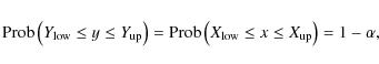
the first-order approximation of the standard deviation is inaccurate
can be found particularly at the inflexion points of the visibility
function (
,
deduced from the first-order expansion of the visibility. Evidence that
the first-order approximation of the standard deviation is inaccurate
can be found particularly at the inflexion points of the visibility
function (
![]() ), where this ratio should not drop to zero. One can notice that the second-order Taylor expansion deduced from Eq. (A.2),
), where this ratio should not drop to zero. One can notice that the second-order Taylor expansion deduced from Eq. (A.2),
![\begin{displaymath}%
\sigma^{2}_{{V}_{\rm ud}} \approx 4 \left[ J_{2} \left( x \...
... \right)\right]^2 ~
\left(\frac{\sigma_{\phi}}{\phi}\right)^4,
\end{displaymath}](/articles/aa/full_html/2010/07/aa13686-09/img54.png)
gives negative values of the variance at the same points, which is a clear indication that higher order Taylor expansions would be needed.
Knowing that the amplitude of the first maximum of J2(x) reaches 0.4865 for
![]() (Andrews 1981), we can infer that the visibility uncertainty of the ud-model due to the calibrator diameter uncertainty never exceeds
(Andrews 1981), we can infer that the visibility uncertainty of the ud-model due to the calibrator diameter uncertainty never exceeds
a maximum value that only depends on the relative uncertainty of the angular diameter. It results that, if one wants to get an absolute uncertainty of the science true visibility
If the relative uncertainty of the model diameter is higher than the experimental visibility
absolute error (
![]() >
>
![]() ),
one can still find values of the
calibrator diameter for which the absolute uncertainty of the science
true visibility is dominated by the measurement errors. This can be
achieved by numerical inversion of Eq. (4), in finding the values of the argument x corresponding to model visibility absolute uncertainties lower than a given value of the measurement error
),
one can still find values of the
calibrator diameter for which the absolute uncertainty of the science
true visibility is dominated by the measurement errors. This can be
achieved by numerical inversion of Eq. (4), in finding the values of the argument x corresponding to model visibility absolute uncertainties lower than a given value of the measurement error
![]() ,
for a given diameter relative uncertainty
,
for a given diameter relative uncertainty
![]() .
Because of the quasi-periodic behaviour of
.
Because of the quasi-periodic behaviour of
![]() against x, as shown in the right panel of Fig. 1, many sets of diameter values, enclosing each zero of the
against x, as shown in the right panel of Fig. 1, many sets of diameter values, enclosing each zero of the
![]() function, can fulfil the condition
function, can fulfil the condition
![]()
![]()
![]() .
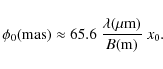
Then, we can define the value x0, below which any ud-calibrator diameter would contribute to the global visibility uncertainty less
than the experimental errors, thanks to the inversion of the relation
.
Then, we can define the value x0, below which any ud-calibrator diameter would contribute to the global visibility uncertainty less
than the experimental errors, thanks to the inversion of the relation
![]() ,
where
,
where ![]() =
=
![]() .
To obtain the corresponding value of the angular diameter
.
To obtain the corresponding value of the angular diameter ![]() ,
we can use Eq. (3)
,
we can use Eq. (3)
For example, if the calibrator angular diameters are estimated with
Table 1:
Values of the angular diameter ![]() (in mas), under which
(in mas), under which
![]() ,
at
,
at
![]() .
.
With B = [330] m,
![]() ,
and
,
and
![]() =
= ![]() ,
we find that any calibrator smaller than [0.42] mas gives
,
we find that any calibrator smaller than [0.42] mas gives
![]() ,
i.e.
,
i.e.
![]() =
=
![]() < 0.02, a result very close to that of van Belle & van Belle (2005), who give [0.45] mas for the same value of
< 0.02, a result very close to that of van Belle & van Belle (2005), who give [0.45] mas for the same value of ![]() .
Figure 2 shows the baselength dependency of
.
Figure 2 shows the baselength dependency of ![]() at wavelengths ofs 10 (upper line), 2.2, 1.25, and [0.7]
at wavelengths ofs 10 (upper line), 2.2, 1.25, and [0.7] ![]() m (lower line) on a log-log scale, with
m (lower line) on a log-log scale, with
![]() and
and
![]() .
.
We can conclude from this short study that the choice of suitable
ud-calibrators for long-baseline optical interferometry depends on the
ratio ![]() of the absolute measurement error of the visibility
of the absolute measurement error of the visibility
![]() to the calibrator angular size prediction error
to the calibrator angular size prediction error
![]() .
If
.
If
![]() ,
any ud-calibrator is suitable, i.e. contributes less than the measurement error
to the global budget error in visibility, because of its angular diameter uncertainty. If
,
any ud-calibrator is suitable, i.e. contributes less than the measurement error
to the global budget error in visibility, because of its angular diameter uncertainty. If ![]() ,
we find that any ud-calibrator with an angular diameter less than a value
,
we find that any ud-calibrator with an angular diameter less than a value ![]() ,
such as
,
such as
![]() ,
is suitable.
,
is suitable.
4 Choosing the calibrators
Choosing calibration targets for a specific scientific programme in a given instrumental configuration is a critical point of the absolute calibration of interferometric measurements. If one wants to determine the visibility of scientific targets with a high degree of accuracy, not only the angular diameters of the calibrators need to be carefully estimated, but also their brightness distributions, which are known to deviate slightly from simple ud-profiles. This implies that suitable calibrators belong to well-known, intensively-studied, and easily-modelled object classes.
As said in Sect. 2, point-like calibrators as bright as their associated scientific targets are ideal interferometric calibrators, which are unfortunately rarely available. Partially resolved sources may also be considered as suitable calibrators, provided that their brightness distribution can be accurately modelled. This excludes irregular and rapid variables, evolved stars, or stellar objects embedded in a complex and varying circumstellar environment involving disks, shells, etc., which are potentially revealed by an infrared excess in the spectral energy distribution (SED).
![\begin{figure}
\par\includegraphics[width=8cm,clip]{13686fg2.eps}
\end{figure}](/articles/aa/full_html/2010/07/aa13686-09/img80.png)
|
Figure 2:
Log-log plot of the angular diameter |
| Open with DEXTER | |
Since we are concerned with studies of the circumstellar environment and of brightness asymmetries on the surface of evolved giants and supergiants, observed at high angular resolution with VLTI-AMBER in the near infrared (NIR), we consider as ``good'' calibrators the celestial targets fulfilling the following criteria:
- 1.
- small angular distance (
![${<}\unit[10]{\hbox{$^\circ$ }}$](/articles/aa/full_html/2010/07/aa13686-09/img81.png) )
to the scientific targets;
)
to the scientific targets;
- 2.
- spectral type not later than K, with luminosity class III at the most (no supergiant nor intrinsically bright giant);
- 3.
- NIR apparent magnitudes as close as possible to the scientific target (
 ,
i.e. flux ratio below 16);
,
i.e. flux ratio below 16);
- 4.
- angular diameter as small as possible but at least smaller than the scientific target;
- 5.
- no near-infrared excess observed in the spectral energy distribution (SED discrepancy with a blackbody radiator within
 in the NIR domain);
- 6.
- no evidence for variability identified in the CDS-SIMBAD database
![[*]](/icons/foot_motif.png) ;
;
- 7.
- preferably source unicity, possibly multiplicity with far (
![${>}\unit[2]{\hbox{$^{\prime\prime}$ }}$](/articles/aa/full_html/2010/07/aa13686-09/img84.png) )
and/or faint (
)
and/or faint (
 )
companion(s) not seen in the observation field of the instrument, thus not affecting interferometric measurements;
)
companion(s) not seen in the observation field of the instrument, thus not affecting interferometric measurements;
- 8.
- no evidence for non centro-symmetric geometry.
The present paper uses the reference giant star ![]() Gru (
Gru (![]() Gruis) as test case,
selected to calibrate the interferometric measurements of the scientific target
Gruis) as test case,
selected to calibrate the interferometric measurements of the scientific target ![]() Gruis (
Gruis (![]() Gruis), that we observed in Oct. 2007 with the VLTI-AMBER instrument. The target
Gruis), that we observed in Oct. 2007 with the VLTI-AMBER instrument. The target ![]() Gru has been used several times as calibrator for interferometry (Kervella et al. 2004; Wittkowski et al. 2006; Di Folco et al. 2004). The following set of basic information can be found for this star:
Gru has been used several times as calibrator for interferometry (Kervella et al. 2004; Wittkowski et al. 2006; Di Folco et al. 2004). The following set of basic information can be found for this star:
- equatorial coordinates (J2000):
 [22] h [06] m [06.885] s,
and
[22] h [06] m [06.885] s,
and
![$\delta= \unit[-39]{\hbox{$^\circ$ }}~\unit[32]{\hbox{$^\prime$ }}~\unit[36.07]{\hbox{$^{\prime\prime}$ }}$](/articles/aa/full_html/2010/07/aa13686-09/img88.png) ;
;
- galactic coordinates (J2000): l =
![$\unit[2.2153]{\hbox{$^\circ$ }}$](/articles/aa/full_html/2010/07/aa13686-09/img89.png) ,
and b =
,
and b =
![$\unit[-53.6743]{\hbox{$^\circ$ }}$](/articles/aa/full_html/2010/07/aa13686-09/img90.png) ;
;
- parallax: [13.20(78)] mas (Perryman et al. 1997);
- spectral type: initially classified as M3III by Buscombe (1962), then as K3III since Houk (1978);
- apparent broadband magnitudes gathered in Table 2;
- infrared fluxes:
 ,
,
 ,
and
,
and
 from IRAS (in Jy) (Beichman et al. 1988);
- infrared spectrophotometry: from 2.38 to [45.21]
 m with ISO-SWS01 (Sloan et al. 2003);
- angular diameter: [2.71(3)] mas (limb-darkened) in the catalogue of calibrator stars for LBSI (Bordé et al. 2002), revised to [2.75(3)] mas by Di Folco et al. (2004) from observations with VLTI/VINCI.
![\begin{figure}
\par\includegraphics[width=8cm,clip]{13686fg3.eps}
\end{figure}](/articles/aa/full_html/2010/07/aa13686-09/img99.png)
|
Figure 3:
Log-log plot of the broadband absolute photometry (in
|
| Open with DEXTER | |
![\begin{figure}
\par\includegraphics[width=8cm,clip]{13686fg4.eps}
\end{figure}](/articles/aa/full_html/2010/07/aa13686-09/img101.png)
|
Figure 4:
Log-log plot of the high-resolution processed SWS01 spectrum (in
|
| Open with DEXTER | |
5 Direct and indirect approaches
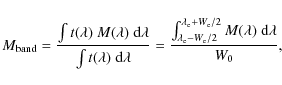
To determine the stellar angular diameters, two different methods are commonly used, classified as direct and indirect by Fracassini et al. (1981). The direct method consists in linking the high angular or spectral resolution observations of some physical phenomena directly with the stellar disk geometry. Unless the instrumental response is known with an extreme accuracy, which is an extremely difficult challenge in the presence of (terrestrial) atmospheric turbulence, the accurate estimation of the calibrator angular diameters with the direct method needs very careful calibration with other unresolved or extremely well-known calibrators. In this case, the problem can be solved thanks to global calibrating strategies (Meisner 2008; Richichi et al. 2009).
The indirect method is based on the luminosity formula
![]() ,
where
,
where
![]() is the linear radius. High-fidelity SED templates (Boden 2007) or stellar atmosphere models can be used to provide homogeneous diameter estimates. Because
of the very small number of existing absolute primary standards (Cohen et al. 1992), indirect diameter estimation needs to beware of the calibration of the absolute flux, hence of the effective temperature.
is the linear radius. High-fidelity SED templates (Boden 2007) or stellar atmosphere models can be used to provide homogeneous diameter estimates. Because
of the very small number of existing absolute primary standards (Cohen et al. 1992), indirect diameter estimation needs to beware of the calibration of the absolute flux, hence of the effective temperature.
The calibrator catalogues of Bordé et al. (2002, hereafter B02), Mérand et al. (2005),
and van Belle et al. (2008) use this method, the first two based on the previous absolute spectral calibration works of Cohen et al. (1999), the latter based on the works of Pickles (1998).
The angular diameter estimates contained in the calibrator catalogue for VLTI-MIDI MCC![]() are also inferred from the indirect method, fitting global photometric
measurements by stellar atmosphere models, giving diameter
uncertainties within
are also inferred from the indirect method, fitting global photometric
measurements by stellar atmosphere models, giving diameter
uncertainties within ![]() 5% (Verhoelst 2005).
5% (Verhoelst 2005).
The compilation of all stellar diameter values published in the literature has been carried out to build the CADARS (Pasinetti Fracassini et al. 2001; Fracassini et al. 1981) and the CHARM/CHARM2 (Richichi & Percheron 2002; Richichi et al. 2005) catalogues. Although this approach seems attractive, because it gives the impression of providing ``reliable'' and well-controlled diameters, a sharper analysis of the data shows that these catalogues are intrinsically heterogeneous, with a precision rarely reaching 5%.
The studies presented in the present paper follow the indirect method of estimating the angular diameters of the interferometric calibrators, comparing the results obtained with various observations: diameter from the spectral type, from the colour index, from the broadband infrared magnitude, from the Johnson photometry, and from the spectral energy distribution. We especially focus attention on determining diameter uncertainties.
6 Model atmospheres
Thanks to the considerable progress made in modelling the stellar
atmospheres, extensive grids of synthetic fluxes and spectra are now
available. To get a summary of the existing synthetic spectra, one
can look, for example, at Carrasco's web page![]() . Among all the stellar atmosphere grids available, we should particularly mention: the ATLAS models
. Among all the stellar atmosphere grids available, we should particularly mention: the ATLAS models![]() (Castelli & Kurucz 2003; Kurucz 1979), the PHOENIX stellar and planetary atmosphere code
(Castelli & Kurucz 2003; Kurucz 1979), the PHOENIX stellar and planetary atmosphere code![]() (Hauschildt 1992; Brott & Hauschildt 2005), and the MARCS stellar
atmosphere models
(Hauschildt 1992; Brott & Hauschildt 2005), and the MARCS stellar
atmosphere models![]() (Gustafsson et al. 1975,2008). These codes have been compared by Kucinskas et al. (2005) for the late-type giants, and Meléndez et al. (2008) have shown the very good agreement between them. Concerning MARCS, Decin et al. (2000) has studied the influence of various stellar parameters on the synthetic spectra.
(Gustafsson et al. 1975,2008). These codes have been compared by Kucinskas et al. (2005) for the late-type giants, and Meléndez et al. (2008) have shown the very good agreement between them. Concerning MARCS, Decin et al. (2000) has studied the influence of various stellar parameters on the synthetic spectra.
Because the MARCS code is particularly suitable for the cool stars (Gustafsson et al. 2003), we naturally opt to use it to model the atmosphere of ![]() Gru. Detailed information about the models can be found on the MARCS web site. The library supplies high-resolution (
Gru. Detailed information about the models can be found on the MARCS web site. The library supplies high-resolution (
![]() )
energy fluxes for
)
energy fluxes for
![]() ,
for a wide grid of spherical atmospheric models, obtained with
,
for a wide grid of spherical atmospheric models, obtained with
![]() (step [100] K or [250] K), surface gravities
(step [100] K or [250] K), surface gravities
![]() (step 0.5), metallicities
(step 0.5), metallicities
![]() (with variable step from 1.0 to [0.25] dex), stellar masses
(with variable step from 1.0 to [0.25] dex), stellar masses
![]() of 0.5, 1.0, 2.0, and [5.0]
of 0.5, 1.0, 2.0, and [5.0]
![]() ,
and microturbulent velocity
,
and microturbulent velocity
![]() or
or
![]() .
Figure 5 shows the high-resolution synthetic spectral radiant exitance of a typical K3III star, with
.
Figure 5 shows the high-resolution synthetic spectral radiant exitance of a typical K3III star, with
![]() ,
,
![]() ,
,
![]() ,
,
![]() ,
and
,
and
![]() ,
given by the spherical MARCS model.
,
given by the spherical MARCS model.
![\begin{figure}
\par\includegraphics[width=8cm,clip]{13686fg5.eps}
\end{figure}](/articles/aa/full_html/2010/07/aa13686-09/img119.png)
|
Figure 5:
High-resolution (R=20 000) MARCS synthetic spectral radiant exitance (in
|
| Open with DEXTER | |
![\begin{figure}
\par\includegraphics[width=15cm,clip]{13686fg6.eps}
\end{figure}](/articles/aa/full_html/2010/07/aa13686-09/img120.png)
|
Figure 6:
Median-resolution (R=1000) TURBOSPECTRUM synthetic radiance data,
obtained with the same model parameters as for Fig. 5. Upper left panel: spectral distribution of the central radiance. Upper right panel: spectral distribution of the radiance normalized to the centre, for r=0.345 (upper curve), 0.515, 0.631, 0.720, 0.791, 0.848, 0.883, 0.922, 0.952, 0.974, 0.990, and 0.998 (lower curve). Lower left panel: normalized radiance profiles, for the wavelengths
|
| Open with DEXTER | |
Figure 6 shows the synthetic spectral radiance, obtained with the same set of physical parameters using the TURBOSPECTRUM code (Alvarez & Plez 1998),
with a spectral step of [20] Å. In the upper left panel,
the radiance spectral distribution at the disk centre is shown for
![]() .
The upper right panel shows the radiance normalized to the centre, for various values of the distance from the star centre r
(expressed in photospheric radius units). The model reproduces the
change from absorption (on the disk) to emission (just beyond the
continuum limb) of the first overtone ro-vibrational CO band
at [2.3]
.
The upper right panel shows the radiance normalized to the centre, for various values of the distance from the star centre r
(expressed in photospheric radius units). The model reproduces the
change from absorption (on the disk) to emission (just beyond the
continuum limb) of the first overtone ro-vibrational CO band
at [2.3] ![]() m, also seen in the near-infrared solar observations (Prasad 1998).
The lower left panel shows the normalized radiance profiles for various
wavelengths. The position of the inflexion point gives the
wavelength-independent Rosseland to limb-darkened conversion factor
m, also seen in the near-infrared solar observations (Prasad 1998).
The lower left panel shows the normalized radiance profiles for various
wavelengths. The position of the inflexion point gives the
wavelength-independent Rosseland to limb-darkened conversion factor
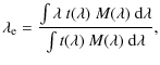
![]() = 1)/
= 1)/
![]() ,
where
,
where
![]() is the model outermost linear diameter (Wittkowski et al. 2004). For a discussion of the different definitions of the stellar radius, one can refer to Baschek et al. (1991). The lower right panel shows first partial derivatives with respect to r of the normalized radiance, against the viewing angle cosine
is the model outermost linear diameter (Wittkowski et al. 2004). For a discussion of the different definitions of the stellar radius, one can refer to Baschek et al. (1991). The lower right panel shows first partial derivatives with respect to r of the normalized radiance, against the viewing angle cosine
![]() .
The median value 0.991 of the inflexion point is very close to the value
.
The median value 0.991 of the inflexion point is very close to the value
![]() predicted by the MARCS code.
predicted by the MARCS code.
For comparison purpose, we use the Planck and the Engelke (Engelke 1992; Marengo 2000)
formulae. Representing the simplest way to model a stellar flux, the
Planck function describes the exitance of a blackbody radiator with
temperature T. Improving upon the blackbody description of
the cool star infrared emission by incorporating empirical corrections
for the main atmospheric effects, the Engelke function is obtained
by substituting T with
![]() in the expression of the Planck formula (T in K and
in the expression of the Planck formula (T in K and ![]() in
in ![]() m). Because it is an analytical approximation of the [2-60]
m). Because it is an analytical approximation of the [2-60] ![]() m continuum spectrum for giants and dwarfs with
m continuum spectrum for giants and dwarfs with
![]() ,
the Engelke function is based on the scaling of a semi-empirical
plane-parallel solar atmospheric exitance profile for various effective
temperatures (Decin & Eriksson 2007).
,
the Engelke function is based on the scaling of a semi-empirical
plane-parallel solar atmospheric exitance profile for various effective
temperatures (Decin & Eriksson 2007).
7 Diameter estimation
Among all the indirect approaches used to estimate the angular diameter, we compare now some of the most widely used methods.
7.1 From the spectral type
The stellar fundamental parameters mass
![]() ,
linear radius
,
linear radius
![]() ,
and absolute luminosity
,
and absolute luminosity
![]() are directly related to the stellar atmospheric parameters effective temperature
are directly related to the stellar atmospheric parameters effective temperature ![]() ,
surface gravity g, according to the logarithmic formulae (Smalley 2005; Straizys & Kuriliene 1981):
,
surface gravity g, according to the logarithmic formulae (Smalley 2005; Straizys & Kuriliene 1981):
This uses the solar parameter values
To estimate the effective temperature and the luminosity from the Morgan-Keenan-Kellman (MKK) type,
de Jager & Nieuwenhuijzen (1987) introduce the continuous variables s (linked to the spectral class) and b (linked to the luminosity) and derive mathematical expressions of
![]() and
and
![]() against s and b, with 1
against s and b, with 1![]() values of 0.021 and 0.164 respectively.
values of 0.021 and 0.164 respectively.
For a K3III star, with s=5.8 and b=3.0, the two-dimensional B-spline interpolation of the tables of de Jager & Nieuwenhuijzen (1987) gives
![]() and
and
![]() ,
hence
,
hence
![]() ,
so that Eq. (9) gives
,
so that Eq. (9) gives
![]() .
To avoid the bias on the distance appearing from the inversion of the parallax (Luri & Arenou 1997; Brown et al. 1997), we deduce the angular diameter
.
To avoid the bias on the distance appearing from the inversion of the parallax (Luri & Arenou 1997; Brown et al. 1997), we deduce the angular diameter ![]() from the linear radius
from the linear radius
![]() and from the parallax
and from the parallax ![]() (
(![]() and
and ![]() in same units),
according to the relation (Allende Prieto 2001)
in same units),
according to the relation (Allende Prieto 2001)
based on the latest value of the angular diameter of the Sun seen at 1 pc:
If the relative uncertainty on
The angular diameter estimate given by this method clearly
underestimates the B02 value ([2.71] mas). An incorrect
parallax value given by Hipparcos cannot be suspected, considering the
relative proximity of ![]() Gru,
located at [76(4)] pc. Slight errors in determining the
luminosity class could be a more likely cause of bias in diameter
estimation. For
Gru,
located at [76(4)] pc. Slight errors in determining the
luminosity class could be a more likely cause of bias in diameter
estimation. For ![]() Gru, we find that a luminosity
Gru, we find that a luminosity
![]() would be more adequate than
would be more adequate than
![]() ,
giving
,
giving
![]() .
.
7.2 From the colour index
Because the accurate stellar classification is a very difficult challenge leading to potential misclassifications, other parameters must be used to investigate the relation between the stellar temperature and the angular size. Being relatively independent of stellar gravities and abundances, the NIR colours are very good temperature indicators (Bell & Gustafsson 1989). For cool stars, the V-K colour index is also known to be the most appropriate parameter for representing the apparent bolometric flux, almost independently of their luminosity class (di Benedetto 1993; Johnson 1966), The empirical derivation of the angular sizes from the colour indices have been studied by many authors (van Belle 1999; di Benedetto 1998; Groenewegen 2004), leading to different relations. For our study, we use the following relations proposed by van Belle et al. (1999), particularly suitable for late-type giants and supergiants
The average standard deviations are: [250] K on ![]() ,
and 30% on
,
and 30% on
![]() .
One of the major difficulties with this method is the correction of the
colour index for the interstellar absorption. Appendix B briefly describes the de-reddening process used in our study. Table 2 gives the results of the correction for the interstellar extinction in the Johnson and in the 2MASS bands. The UBVRI magnitudes come from the JP11 Catalogue (Morel & Magnenat 1978). Because data precision may vary
significantly (Nagy & Hill 1980), a conservative value of 0.05 has been arbitrarily chosen as the uncertainty on each magnitude. The JHK
.
One of the major difficulties with this method is the correction of the
colour index for the interstellar absorption. Appendix B briefly describes the de-reddening process used in our study. Table 2 gives the results of the correction for the interstellar extinction in the Johnson and in the 2MASS bands. The UBVRI magnitudes come from the JP11 Catalogue (Morel & Magnenat 1978). Because data precision may vary
significantly (Nagy & Hill 1980), a conservative value of 0.05 has been arbitrarily chosen as the uncertainty on each magnitude. The JHK
![]() magnitudes and uncertainties are taken from the 2MASS Catalogue (Cutri et al. 2003).
magnitudes and uncertainties are taken from the 2MASS Catalogue (Cutri et al. 2003).
Table 2:
Broadband photometry of ![]() Gru and reddening.
Gru and reddening.
Using the corrected (intrinsic) V-K colour index 3.16(29) deduced from Table 2, we can infer from Eqs. (13) and (14) that the effective temperature of ![]() Gru is [4247(250)] K, and the linear radius is [26.6(80)]
Gru is [4247(250)] K, and the linear radius is [26.6(80)]
![]() .
Since the linear radius relative uncertainty is 30%, we estimate
the angular diameter uncertainty range according to the CITP.
.
Since the linear radius relative uncertainty is 30%, we estimate
the angular diameter uncertainty range according to the CITP.
As a result, with the parallax [13.20(78)] mas, the V-K angular diameter is [3.3(10)] mas, slightly greater than the B02 value [2.71] mas. A V-K value 2.92 would give an angular diameter estimate closer to the B02. Unfortunately, the high level of final uncertainties prevent knowing the most likely source of bias: errors on the input magnitudes, de-reddening process, or diameter estimation method itself.
The angular diameter estimation given by the JMMC-SearchCal tool is, for bright objects (Bonneau et al. 2006), based on the study undertaken by Delfosse (2004), where a least-square polynomial fit of the distance-independent diameter estimator
![]() against each deredenned colour index CI is achieved. Introducing the distance modulus
against each deredenned colour index CI is achieved. Introducing the distance modulus
![]() (with
(with ![]() in arcsec) in Eq. (11), where mV and MV are the apparent and the absolute stellar magnitudes in V, one can define
in arcsec) in Eq. (11), where mV and MV are the apparent and the absolute stellar magnitudes in V, one can define ![]() by
by
for ![]() in mas. Among the empirical relations between
in mas. Among the empirical relations between ![]() and each colour index, the highest accuracies on the angular diameter
and each colour index, the highest accuracies on the angular diameter ![]() given by Eq. (15) are obtained with the three colour indices B-V (
given by Eq. (15) are obtained with the three colour indices B-V (
![]() ,
for
,
for
![]() ), V-R (10%, for
), V-R (10%, for
![]() ), and V-K (7%, for
), and V-K (7%, for
![]() ). Unlike the classical methods of angular diameter estimation from the colour index, as the method of van Belle et al. (1999),
which needs a parallax estimate in complement to magnitude measurements
in 2 bands, Bonneau's method needs only photometric data, more
precisely the apparent V magnitude and the colour indices. With
B-V = 1.36(25),
V-R = 0.99(19), and
V-K = 3.16(21), the corresponding angular diameter estimates of
). Unlike the classical methods of angular diameter estimation from the colour index, as the method of van Belle et al. (1999),
which needs a parallax estimate in complement to magnitude measurements
in 2 bands, Bonneau's method needs only photometric data, more
precisely the apparent V magnitude and the colour indices. With
B-V = 1.36(25),
V-R = 0.99(19), and
V-K = 3.16(21), the corresponding angular diameter estimates of ![]() Gru are
Gru are
![]() ,
,
![]() ,
and
,
and
![]() .
Although this method gives coherent diameter estimates within
.
Although this method gives coherent diameter estimates within ![]() 11%, which confirms that SearchCal considers
11%, which confirms that SearchCal considers ![]() Gru
as a suitable calibrator for interferometry, it also overestimates
the B02 value [2.71] mas, especially using the B-V colour
index. For a K3 giant, the fiducial Johnson colours taken from
spectral type-luminosity class-colour relations given by Bonneau et al. (2006), would be: B-V=1.27, V-R=0.98, and V-K=3.01. With these colour indices, the angular diameter estimates would be:
Gru
as a suitable calibrator for interferometry, it also overestimates
the B02 value [2.71] mas, especially using the B-V colour
index. For a K3 giant, the fiducial Johnson colours taken from
spectral type-luminosity class-colour relations given by Bonneau et al. (2006), would be: B-V=1.27, V-R=0.98, and V-K=3.01. With these colour indices, the angular diameter estimates would be:
![]() ,
,
![]() ,
and
,
and
![]() ,
close to the B02 value. At least 3 causes of bias may be suspected:
,
close to the B02 value. At least 3 causes of bias may be suspected:
- 1.
- Decreasing the B corrected magnitude from 5.79 to 5.70 would be sufficient to lower the B-V angular diameter estimate to [2.94] mas, so that the diameter estimates in B-V, V-R, and V-K, would stay within
 2%. Thus, a slight overestimate of the B magnitude of Gru in the JP11 catalogue may be suspected.
- 2.
- On the other hand, tests of the de-reddening procedure show that, even if we artificially increase the visual extinction from 0.04 to an unrealistically high value of 2.0 mag, the angular diameter derived from B-V would decrease from 3.32 to barely [3.30] mas, while the V-R and the V-K diameters would get closer to the B02 value, respectively from 2.97 to [2.65] mas, and from to 3.01 to [2.84] mas.
- 3.
- Since the intrinsic B-V colour index of Gru (1.36)
is slightly larger than the upper limit (1.30) of the validity
domain of the polynomial fit, it is finally not surprising that
the method gives an incorrect diameter estimate from B-V in this case.
7.3 From the in-band magnitude
The two methods for estimating the stellar diameter presented above are
based on statistical relations and do not use any photospheric model.
On the contrary, the methods presented in the following sections
explicitly need photospheric models. As first shown by Blackwell & Shallis (1977),
the photometric angular diameter in a spectral band can be estimated thanks to the relation
![]() ,
where
,
where
![]() and
and
![]() are the received and emergent mean fluxes in the considered band (both in
are the received and emergent mean fluxes in the considered band (both in
![]() ).
The angular diameters derived with this method, known as the infra-red
flux method (IRFM), are generally accurate to between 2
and 3% (Blackwell et al. 1990),
depending not only on the fidelity of the atmospheric models used in
the calibration, but also on the uncertainty in the absolute flux
determination.
).
The angular diameters derived with this method, known as the infra-red
flux method (IRFM), are generally accurate to between 2
and 3% (Blackwell et al. 1990),
depending not only on the fidelity of the atmospheric models used in
the calibration, but also on the uncertainty in the absolute flux
determination.
The last column of Table 2 lists the received absolute fluxes deduced from the measured de-reddened in-band magnitudes
![]() ,
where F0 is the zero-magnitude flux taken from Bessell et al. (1998) for UBVRI, with 2% uncertainties (Colina et al. 1996), and from Cohen et al. (2003) for JHK
,
where F0 is the zero-magnitude flux taken from Bessell et al. (1998) for UBVRI, with 2% uncertainties (Colina et al. 1996), and from Cohen et al. (2003) for JHK
![]() .
For in-band corrected magnitudes with relative uncertainties
exceeding 20%, absolute flux uncertainties are computed according
to the CITP (see Eq. (A.3)).
.
For in-band corrected magnitudes with relative uncertainties
exceeding 20%, absolute flux uncertainties are computed according
to the CITP (see Eq. (A.3)).
If
![]() is the transmission profile of the considered filter, normalized
to 1.0 at its maximum, one can define the in-band effective
wavelength and width as (Fiorucci & Munari 2003)
is the transmission profile of the considered filter, normalized
to 1.0 at its maximum, one can define the in-band effective
wavelength and width as (Fiorucci & Munari 2003)
so that the band emergent mean flux
where
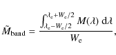
the in-band angular diameter is given by
Table 3:
Effective wavelength and bandwidth (in square brackets) in each band (both in ![]() m), for a K2 spectral type spectrum and a [4250] K blackbody spectrum.
m), for a K2 spectral type spectrum and a [4250] K blackbody spectrum.
Table 4: Photometric angular diameters (in mas) obtained with various synthetic spectra (with T = [4250] K) in the 2MASS near-infrared bands.
Given for comparison, the overestimated angular diameters obtained with the Planck spectrum
confirm that the stellar photospheres may deviate noticeably from simple blackbodies. Similarly,
the underestimated J-band angular diameter derived from the Engelke spectrum confirms that
the Engelke analytic approximation is valid for wavelengths longer than [2] ![]() m. Finally, the MARCS synthetic spectrum with
m. Finally, the MARCS synthetic spectrum with
![]() ,
,
![]() ,
,
![]() ,
,
![]() ,
and
,
and
![]() yields angular diameters in J, H, and
yields angular diameters in J, H, and ![]() ,
which are close to the B02 value of [2.71] mas, and with less dispersion.
,
which are close to the B02 value of [2.71] mas, and with less dispersion.
7.4 From the broadband photometry
The IRFM method, described in Sect. 7.3,
gives different angular-diameter estimates for each spectral band in
which the model spectrum is integrated. To get a unique estimate
of the angular diameter, taking the global broadband photometry into
account (as shown for example in Fig. 3), the use of fitting techniques is necessary. The most widely used is based on ![]() minimization.
minimization.
If
![]() is the measurement error of the mean flux Fi, received in spectral
band i, and Mi the emergent mean flux in the same band, the best-fit angular diameter corresponds to the minimum of the one-parameter
is the measurement error of the mean flux Fi, received in spectral
band i, and Mi the emergent mean flux in the same band, the best-fit angular diameter corresponds to the minimum of the one-parameter ![]() (
(![]() )
nonlinear function defined by
)
nonlinear function defined by
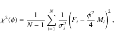
where N is the total number of spectral bands used to build the global photometry. To find the minimum value of the ![]() function,
we use the gradient-expansion algorithm, which combines the features of
the gradient search with the method of linearizing the fitting function
(Bevington & Robinson 1992), very similar to the classical Levenberg-Marquardt algorithm (Levenberg 1944; Marquardt 1963). Figure 7 shows an example of
function,
we use the gradient-expansion algorithm, which combines the features of
the gradient search with the method of linearizing the fitting function
(Bevington & Robinson 1992), very similar to the classical Levenberg-Marquardt algorithm (Levenberg 1944; Marquardt 1963). Figure 7 shows an example of ![]() against the angular diameter obtained when fitting the MARCS model
on the ISO SWS data, as described in Sect. 7.5, using the gradient-expansion algorithm. First used by Cohen et al. (1992)
for the absolute calibration of broad- and narrow-band infrared
photometry, based upon the Kurucz stellar models of Vega and Sirius,
this method has led to the construction of a self-consistent, all-sky
network of over 430 infrared radiometric calibrators (Cohen et al. 1999), upon which
the further works of B02 and Mérand et al. (2005)
are based. Estimating the stellar angular diameters through photometric
modelling is also used in the MSC-getCal Interferometric Observation
Planning Tool Suite, which relies on the Planck blackbody SED,
parameterized by its effective temperature and bolometric flux
(see the fbol routine in the reference manual available online
against the angular diameter obtained when fitting the MARCS model
on the ISO SWS data, as described in Sect. 7.5, using the gradient-expansion algorithm. First used by Cohen et al. (1992)
for the absolute calibration of broad- and narrow-band infrared
photometry, based upon the Kurucz stellar models of Vega and Sirius,
this method has led to the construction of a self-consistent, all-sky
network of over 430 infrared radiometric calibrators (Cohen et al. 1999), upon which
the further works of B02 and Mérand et al. (2005)
are based. Estimating the stellar angular diameters through photometric
modelling is also used in the MSC-getCal Interferometric Observation
Planning Tool Suite, which relies on the Planck blackbody SED,
parameterized by its effective temperature and bolometric flux
(see the fbol routine in the reference manual available online![]() ).
).
![\begin{figure}
\par\includegraphics[width=7cm,clip]{13686fg7.eps}
\end{figure}](/articles/aa/full_html/2010/07/aa13686-09/img199.png)
|
Figure 7:
Plot of |
| Open with DEXTER | |
Table 5: Angular diameters obtained by fitting various models (with T = [4250] K) to visible and/or NIR photometric data.
Table 5 gives the results of the fitting process for the visible and/or NIR photometry (given in Table 2),
with the Planck, the Engelke (suitable for infrared wavelengths only),
and the MARCS models. Since the blackbody model ignores
line-blanketing effects in the near-UV (Allende Prieto & Lambert 2000), as seen in Fig. 3, the Johnson-U flux is not considered when fitting the Planck model. The best-fit angular diameters correspond to the minimum values of the ![]() function. To compare the
function. To compare the
![]() values obtained for
data samples with different sizes, it is convenient to use the F2 goodness-of-fit parameter defined as (Kovalevsky & Seidelmann 2004)
values obtained for
data samples with different sizes, it is convenient to use the F2 goodness-of-fit parameter defined as (Kovalevsky & Seidelmann 2004)
![\begin{displaymath}%
F2 = \left( \frac{9 \nu}{2} \right)^{1/2} \left[ \left( \frac{\chi^{2}}{\nu} \right)^{1/3}
+ \frac{2}{9 \nu} - 1 \right],
\end{displaymath}](/articles/aa/full_html/2010/07/aa13686-09/img207.png)
where
As underlined by Press et al. (2007), although ![]() minimization
is a useful way of estimating the parameters, the formal
covariance matrix of the output parameters has a clear quantitative
interpretation only if the measurement uncertainties are normally
distributed. To derive robust estimates of the model parameter
uncertainties, we used the confidence limits of the fitted parameters
with the bootstrap method (Efron 1979,1982).
Rather than resampling the individual observations with replacement, we
use the method of residual resampling, more relevant for regression,
as described in Appendix C.
minimization
is a useful way of estimating the parameters, the formal
covariance matrix of the output parameters has a clear quantitative
interpretation only if the measurement uncertainties are normally
distributed. To derive robust estimates of the model parameter
uncertainties, we used the confidence limits of the fitted parameters
with the bootstrap method (Efron 1979,1982).
Rather than resampling the individual observations with replacement, we
use the method of residual resampling, more relevant for regression,
as described in Appendix C.
In Table 5, the 68% confidence interval limits of the best-fit angular diameter are determined by bootstrap, with 1000 resampling loops, only for data sets containing more than 5 photometric bands. Although the angular diameters listed in Table 5 (obtained by fitting model fluxes on photometric measurements) are very close to those obtained from the IRFM method, we did not consider the former results as very robust, considering the small number of photometric bands used for the fits.
7.5 From the spectrophotometry
Fitting atmospheric models on sparse photometric data may result in
large uncertainties on the angular diameter. To decrease them
significantly, larger data sets are needed. The observational data for
this section consist in spectro-photometric measurements obtained with
ISO-SWS (de Graauw et al. 1996). The ![]() Gru spectrum shown in Fig. 4,
extracted from the NASA/IPAC Infrared Science Archive, was obtained in
the SWS01 observing mode (low-resolution full grating scan, on-target
time = [1140] s), which covers the entire
2.4-[45.4]
Gru spectrum shown in Fig. 4,
extracted from the NASA/IPAC Infrared Science Archive, was obtained in
the SWS01 observing mode (low-resolution full grating scan, on-target
time = [1140] s), which covers the entire
2.4-[45.4] ![]() m SWS spectral range, with a variable spectral resolution (Table 6). The SWS AOT-1 spectra, subdivided into wavelength segments (Leech et al. 2003), have been processed and renormalized with the post-pipeline algorithm referred as the swsmake code (Sloan et al. 2003). The spectral characteristics of the SWS AOT-1 bands and their 1
m SWS spectral range, with a variable spectral resolution (Table 6). The SWS AOT-1 spectra, subdivided into wavelength segments (Leech et al. 2003), have been processed and renormalized with the post-pipeline algorithm referred as the swsmake code (Sloan et al. 2003). The spectral characteristics of the SWS AOT-1 bands and their 1![]() photometric accuracies given in Table 6 were deduced from Leech et al. (2003) and Lorente (1998). Since the spectrum of
photometric accuracies given in Table 6 were deduced from Leech et al. (2003) and Lorente (1998). Since the spectrum of ![]() Gru is very noisy at wavelengths longer than [27.5]
Gru is very noisy at wavelengths longer than [27.5] ![]() m, as shown in Fig. 4, probably because of calibration problems,
we did not use the bands 3E and 4 for fitting the models on the ISO-SWS data.
m, as shown in Fig. 4, probably because of calibration problems,
we did not use the bands 3E and 4 for fitting the models on the ISO-SWS data.
Table 6: Spectral characteristics of the SWS AOT-1 bands and their photometric accuracy.
Table 7:
Angular diameters obtained by fitting various models (with T = [4250] K) to the 2.38-[27.5] ![]() m SWS spectrum.
m SWS spectrum.
Table 7 gives the results of the fitting process of the SWS 2.38-[27.5] ![]() m
spectrum with the Planck and Engelke models (both with a temperature of
[4250] K) and with the K3III MARCS model, presented in
Sect. 6. The confidence interval limits were estimated using the bootstrap resampling (
m
spectrum with the Planck and Engelke models (both with a temperature of
[4250] K) and with the K3III MARCS model, presented in
Sect. 6. The confidence interval limits were estimated using the bootstrap resampling (
![]() )
for the 68% confidence level. The agreement between the angular
diameter obtained by spectrophotometry fitting with the
MARCS model and the B02 value, obtained by fitting with the
Kurucz model, reflects the excellent agreement between the two models (Meléndez et al. 2008). Deriving the angular diameters from the fit of the Engelke function on the SWS spectra (extended to [45.2]
)
for the 68% confidence level. The agreement between the angular
diameter obtained by spectrophotometry fitting with the
MARCS model and the B02 value, obtained by fitting with the
Kurucz model, reflects the excellent agreement between the two models (Meléndez et al. 2008). Deriving the angular diameters from the fit of the Engelke function on the SWS spectra (extended to [45.2] ![]() m), Heras et al. (2002)
gives an overestimated value of the angular diameter
([2.82(21)] mas, as compared to 2.71(3) from B02).
Figure 8 shows a typical
example of the histogram of the residual-bootstrap estimates of the
best-fit angular diameter, obtained with the MARCS model on the
SWS AOT-1 data, where one can see that the resulting distribution of
angular diameters is notably asymmetric.
m), Heras et al. (2002)
gives an overestimated value of the angular diameter
([2.82(21)] mas, as compared to 2.71(3) from B02).
Figure 8 shows a typical
example of the histogram of the residual-bootstrap estimates of the
best-fit angular diameter, obtained with the MARCS model on the
SWS AOT-1 data, where one can see that the resulting distribution of
angular diameters is notably asymmetric.
![\begin{figure}
\par\includegraphics[width=7cm,clip]{13686fg8.eps}
\end{figure}](/articles/aa/full_html/2010/07/aa13686-09/img212.png)
|
Figure 8: Histogram of the angular diameters estimated by residual bootstrapping when fitting the MARCS model on the SWS spectrum. |
| Open with DEXTER | |
8 Discussion
8.1 Diameter uncertainty
![\begin{figure}
\par\includegraphics[width=8.8cm,clip]{13686fg9.eps}
\end{figure}](/articles/aa/full_html/2010/07/aa13686-09/img213.png)
|
Figure 9:
Estimated sizes of |
| Open with DEXTER | |
Figure 9 summarizes the angular diameter estimates of the test-case calibrator ![]() Gru,
obtained in the present study using various data types and methods. The
B02 value of [2.71] mas is given for comparison. The last
method (estimating the angular diameter from a fit of the
SWS spectrum with a MARCS model gives, as expected, the
most reliable estimate of the angular diameter, very close to the B02
estimate, with an uncertainty of 2.7%. It is also noticeable
that the weighted average of the 23 angular diameter estimates
is [2.73] mas.
Gru,
obtained in the present study using various data types and methods. The
B02 value of [2.71] mas is given for comparison. The last
method (estimating the angular diameter from a fit of the
SWS spectrum with a MARCS model gives, as expected, the
most reliable estimate of the angular diameter, very close to the B02
estimate, with an uncertainty of 2.7%. It is also noticeable
that the weighted average of the 23 angular diameter estimates
is [2.73] mas.
We must underline that the uncertainty of the limb-darkened angular diameter given by B02 is deduced from the formal standard error associated with the best-fit value of the multiplicative factor, scaling the appropriate Kurucz model on the infrared fluxes (Cohen et al. 1996). Called biases by Cohen et al. (1995), scale factor uncertainties rarely reach 1% with their method, independent of the spectral type and luminosity class. If we use, in the same manner, the formal fit errors as uncertainty estimators, the diameter uncertainty only amounts to 0.15%. Since we consider this extremely low value as unrealistic, we prefer to estimate the angular-diameter uncertainty from the statistically-significant confidence intervals, given by the residual bootstrapping (Appendix C). This amounts to 2.4% with the fit of the MARCS model.
8.2 Fundamental stellar parameters
From this angular-diameter accurate estimate and the parallax, we can infer a set of fundamental stellar parameters for ![]() Gru, presented in Table 8, using the following procedure.
Gru, presented in Table 8, using the following procedure.
- 1.
- Calculate the linear radius
 from
from  and
and  ,
according to Eq. (11). For
,
according to Eq. (11). For
![$\phi = \unit[2.70]~{\rm mas}$](/articles/aa/full_html/2010/07/aa13686-09/img214.png) and
and
![$\varpi = \unit[13.20]~{\rm mas}$](/articles/aa/full_html/2010/07/aa13686-09/img215.png) ,
we find
,
we find
![$\mathcal{R} = \unit[22.0]~{\mathcal{R_{\odot}}}$](/articles/aa/full_html/2010/07/aa13686-09/img216.png) .
.
- 2.
- Fix the value of the spectral class variable s from the spectral type. For a K3 star, s=5.80.
- 3.
- Find the value of the luminosity class variable b, which gives the same angular diameter value. One can easily demonstrate from Eq. (12) that b is solution of the equation
where t(s,b) and l(s,b) are the two-dimensional B-spline interpolation functions of the tables and
and
 ,
published by de Jager & Nieuwenhuijzen (1987). For
and
,
we find b = 2.76.
,
published by de Jager & Nieuwenhuijzen (1987). For
and
,
we find b = 2.76.
- 4.
- From s=5.80 and b=2.76, deduce the interpolated effective temperature
 and the absolute luminosity
 ,
and calculate the bolometric magnitude
,
and calculate the bolometric magnitude
 .
.
- 5.
- Interpolate the surface gravity
 in the corresponding table of Straizys & Kuriliene (1981)
for the same couple of values (s,b).
in the corresponding table of Straizys & Kuriliene (1981)
for the same couple of values (s,b).
- 6.
- Using Eq. (10), deduce the stellar mass
 from
and .
from
and .
Table 8:
Fundamental parameter estimates (with uncertainties) of ![]() Gru reevaluated from our study.
Gru reevaluated from our study.
Using this method, one can see from Table 8
that the bolometric magnitude and especially the stellar mass are
determined with very low accuracies. The fundamental parameter
accuracies are computed using the 1![]() accuracies given by de Jager & Nieuwenhuijzen (1987): 0.021 for
accuracies given by de Jager & Nieuwenhuijzen (1987): 0.021 for
![]() ,
0.164 for
,
0.164 for
![]() ,
and 0.4 for
,
and 0.4 for ![]() .
The uncertainties on the fundamental parameters deduced by our study
validate a posteriori the choice of the input parameter values for
the MARCS model used to fit the flux measurements:
.
The uncertainties on the fundamental parameters deduced by our study
validate a posteriori the choice of the input parameter values for
the MARCS model used to fit the flux measurements:
![]() ,
,
![]() ,
and
,
and
![]() .
.
8.3 Model parameters
One critical point of our method is the preliminary choice of a single
set of photospheric model parameters, used to infer the angular
diameter. To determine them accurately, we refer the reader to the
papers by Decin et al. (2000) and Decin et al. (2004). In our study, we use the MARCS model with the fiducial parameter set of a K3III star, i.e.
![]() ,
,
![]() ,
,
![]() ,
,
![]() ,
and
,
and
![]() .
The very good agreement between the angular diameter estimates deduced
from the fit of the Planck, the Engelke and the MARCS models on
the ISO-SWS 2.38-[27.5]
.
The very good agreement between the angular diameter estimates deduced
from the fit of the Planck, the Engelke and the MARCS models on
the ISO-SWS 2.38-[27.5] ![]() m spectrum of
m spectrum of ![]() Gru, as it is shown in Table 7, justifies the choice of these model parameters.
Gru, as it is shown in Table 7, justifies the choice of these model parameters.
9 Conclusion
In our paper, we have compared different methods for angular-diameter estimation of the interferometric calibrators. The spectral-type angular diameters only need distances as extra input. The colour-index diameters need a good interstellar correction. The photometric and the spectrophotometric diameters need explicit synthetic spectra. As expected, the results are highly dependent on the number and quality of the input data.
As a test case, we used the giant cool star ![]() Gru that we observed to calibrate the VLTI-AMBER low-resolution
Gru that we observed to calibrate the VLTI-AMBER low-resolution ![]() observations
observations![]() of the scientific target
of the scientific target ![]() Gru (Sacuto et al. 2008), which will be the subject of our forthcoming paper.
Gru (Sacuto et al. 2008), which will be the subject of our forthcoming paper.
Each diameter estimate is compared to the B02 value ([2.71] mas)
found in the Calalogue of Calibrator Stars for Interferometry. The most
reliable estimate of the angular diameter we find is [2.70] mas,
with a 68% confidence interval [2.65-2.81] mas, obtained
by fitting the ISO/SWS spectrum (2.38-[27.5] ![]() m) with a MARCS atmospheric model, characterized by
m) with a MARCS atmospheric model, characterized by
![]() ,
,
![]() ,
,
![]() ,
,
![]() ,
and
,
and
![]() .
One original contribution of our study is the estimation of the
statistically-significant uncertainties by means of the unbiased
confidence intervals, determined by residual bootstrapping.
.
One original contribution of our study is the estimation of the
statistically-significant uncertainties by means of the unbiased
confidence intervals, determined by residual bootstrapping.
All numerical results and graphical outputs presented in the paper were obtained using the
routines developed under PV-WAVE, which compose the modular software suite
SPIDAST![]() ,
created to calibrate and interpret spectroscopic and interferometric
measurements, particularly those obtained with VLTI-AMBER (Cruzalèbes et al. 2008). The main functionalities of the SPIDAST code, intended to be available to the community, are
,
created to calibrate and interpret spectroscopic and interferometric
measurements, particularly those obtained with VLTI-AMBER (Cruzalèbes et al. 2008). The main functionalities of the SPIDAST code, intended to be available to the community, are
- 1.
- estimate the calibrator angular diameter by any of the methods described in this paper;
- 2.
- create calibrator synthetic measurements, for the instrumental configuration (spectral fluxes, visibilities, and closure phases);
- 3.
- estimate the instrumental response from the observational and the synthetic measurements of the calibrator;
- 4.
- calibrate the observational measurements of the scientific target with the instrumental response;
- 5.
- determine the science parameters by fitting the chromatic analytic model on the true science measurements, with the confidence intervals given by residual bootstrapping.
P.C. thanks A. Spang, Y. Rabbia, O. Chesneau, and A. Mérand for helpful discussions. A.J. is grateful to B. Plez and T. Masseron for their ongoing support with the MARCS code. S.S. acknowledges funding by the Austrian Science Fund FWF under the project P19503-N13. We also thank the anonymous referee whose comments helped us to improve the clarity of this paper. This research has made use of the Jean-Marie Mariotti Centre SearchCal service, co-developed by FIZEAU and LAOG, of the CDS Astronomical Databases SIMBAD and VIZIER, and of the NASA Astrophysics Data System Abstract Service.
Appendix A: Computing the uncertainties
As defined in the Guide to the Expression of Uncertainty in Measurement (JCGM/WG 1 2008),
the uncertainty
![]() ,
associated to the ``best'' estimate
,
associated to the ``best'' estimate ![]() of a given random variable x, usually given by the sample average, characterizes the dispersion of x about
of a given random variable x, usually given by the sample average, characterizes the dispersion of x about ![]() .
When it is associated to the level of confidence
.
When it is associated to the level of confidence ![]() ,
it can be interpreted as defining the interval around
,
it can be interpreted as defining the interval around ![]() ,
which encompasses 100(
,
which encompasses 100(![]() )% of the estimates X of x. By analogy with the 1
)% of the estimates X of x. By analogy with the 1![]() dispersion in the normal case, one can define the standard uncertainty of
dispersion in the normal case, one can define the standard uncertainty of ![]() by the interval that encompasses 68.3% of the distribution of x around
by the interval that encompasses 68.3% of the distribution of x around ![]() .
.
If
![]() are the right and left deviations of x varying in the 100(
are the right and left deviations of x varying in the 100(![]() )% confidence interval (CI) about
)% confidence interval (CI) about ![]() ,
they can be defined as
,
they can be defined as
![]() and
and
![]() ,
where
,
where
![]() and
and
![]() are the upper and lower bounds of the CI, respectively given by the 100
are the upper and lower bounds of the CI, respectively given by the 100
![]() % and 100
% and 100
![]() % quantiles of the distribution of x.
% quantiles of the distribution of x.
To propagate the uncertainties with a monotonic transformation function f of the input variable x into the output variable
![]() ,
one can follow the confidence interval transformation principle (CITP) (Kelley 2007; Smithson 2002)
,
one can follow the confidence interval transformation principle (CITP) (Kelley 2007; Smithson 2002)
where
The upper and lower output uncertainties can be defined by the left and right deviations of y about its best estimate ![]() ,
so that
,
so that
![]() ,
and
,
and
![]() .
.
For small input uncertainties
![]() ,
one can apply the approximation of a second-order Taylor series expansion to compute the upper/lower output uncertainties
,
one can apply the approximation of a second-order Taylor series expansion to compute the upper/lower output uncertainties
![]() .
Omitting the terms leading to moments higher than the second one, Winzer (2000) gives
.
Omitting the terms leading to moments higher than the second one, Winzer (2000) gives
where
For practical reasons, it is often more convenient to associate a single uncertainty value
![]() ,
hereafter denoted
,
hereafter denoted ![]() in order to simplify the notations, rather than dealing with asymmetric uncertainties
in order to simplify the notations, rather than dealing with asymmetric uncertainties
![]() ,
hereafter denoted
,
hereafter denoted
![]() .
Most people remove the asymmetry by taking the highest value between
.
Most people remove the asymmetry by taking the highest value between
![]() and
and
![]() ,
or by averaging the two values, arithmetically or geometrically.
Although the arithmetic mean gives the correct uncertainty in most
cases of practical interest and small uncertainties (D'Agostini & Raso 2000),
we can follow a statistical approach based on asymmetrical probability
density functions (pdf), also applicable with large uncertainties.
,
or by averaging the two values, arithmetically or geometrically.
Although the arithmetic mean gives the correct uncertainty in most
cases of practical interest and small uncertainties (D'Agostini & Raso 2000),
we can follow a statistical approach based on asymmetrical probability
density functions (pdf), also applicable with large uncertainties.
In the general case where the 100(![]() )% CI does not encompass the whole distribution of the estimates X of x, asymmetric uncertainties need careful handling with known likelihood functions (Barlow 2003). If the CI bounds
)% CI does not encompass the whole distribution of the estimates X of x, asymmetric uncertainties need careful handling with known likelihood functions (Barlow 2003). If the CI bounds
![]() and
and
![]() are close to the extremal values
are close to the extremal values ![]() and
and ![]() of
the distribution, and if there is no specific knowledge about the
distribution itself, one can use the standard deviation of an
asymmetric distribution as estimator for the symmetric uncertainty.
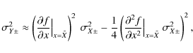
When only the value of the best estimate
of
the distribution, and if there is no specific knowledge about the
distribution itself, one can use the standard deviation of an
asymmetric distribution as estimator for the symmetric uncertainty.
When only the value of the best estimate ![]() is known, in addition to the upper and lower bounds of the CI, it is reasonable to assume that the probability to obtain values near the bounds is lower than values near
is known, in addition to the upper and lower bounds of the CI, it is reasonable to assume that the probability to obtain values near the bounds is lower than values near ![]() .
In this case, a simple approximation of the pdf is given by the asymmetric triangular distribution, with mode
.
In this case, a simple approximation of the pdf is given by the asymmetric triangular distribution, with mode ![]() ,
width
,
width
![]() ,
and variance
,
and variance
![\begin{displaymath}%
\sigma^{2}_{\rm tri} = \frac{\left( X_{\max} - X_{\min}\rig...
... \right)}
{\left( X_{\max} - X_{\min }\right)^2} \right]\cdot
\end{displaymath}](/articles/aa/full_html/2010/07/aa13686-09/img264.png)
Kotz & Van Dorp (2004) give the analytic relations

where q is solution of the equation
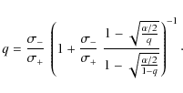
Throughout our study, we use the standard deviation of the asymmetric triangular distribution as estimator for the symmetric uncertainty.
Appendix B: De-reddening
If
![]() is the observed broad-band magnitude, the dereddened magnitude is
is the observed broad-band magnitude, the dereddened magnitude is
![]() ,
where
,
where
![]() is
the interstellar extinction in the band. To calculate the value of
the extinction at any wavelength, we use the relation
is
the interstellar extinction in the band. To calculate the value of
the extinction at any wavelength, we use the relation
![]() ,
where
,
where
![]() is
the ratio of total to selective extinction at any wavelength (Seaton 1979), and V and B stand for the visible and the blue wavelengths:
is
the ratio of total to selective extinction at any wavelength (Seaton 1979), and V and B stand for the visible and the blue wavelengths:
![]() ,
and
,
and
![]() (Williams 1992; Cardelli et al. 1989).
(Williams 1992; Cardelli et al. 1989).
To get the wavelength dependence of the extinction
![]() in the IR/optical region, we use
the tabular data of the Asiago Database of Photometric Systems available online, following Fitzpatrick (1999), for the case
RV = 3.1.
in the IR/optical region, we use
the tabular data of the Asiago Database of Photometric Systems available online, following Fitzpatrick (1999), for the case
RV = 3.1.
The visual interstellar extinction AV is calculated thanks to the numerical algorithm of Hakkila et al. (1997), including the studies of Fitzgerald (1968), Neckel & Klare (1980), Berdnikov & Pavlovskaya (1991), Arenou et al. (1992), Chen et al. (1998), and Drimmel & Spergel (2001), plus a sample of studies of high-galactic latitude clouds. The algorithm calculates the three-dimensional visual extinction from inputs of distance, Galactic longitude and latitude. The final estimate of the visual extinction is given by weighted averaging of the individual study values. Since the datasets used in the analyses are not statistically independent, Hakkila suggests to use the simple averaging of the individual study uncertainties as formal extinction uncertainty.
Table B.1:
Total visual extinction of ![]() Gru as obtained from the relevant studies.
Gru as obtained from the relevant studies.
The total visual extinctions of ![]() Gru are shown in Table B.1 for the relevant studies, with the distance [76] pc, and the Galactic coordinates l =
Gru are shown in Table B.1 for the relevant studies, with the distance [76] pc, and the Galactic coordinates l =
![]() ,
and b =
,
and b =
![]() .
Because the estimate from Arenou et al. (1992) does not agree with the 4 other estimates, we do not use it for averaging.
The weighted average estimate of AV is 0.03, with a mean uncertainty of 0.15.
.
Because the estimate from Arenou et al. (1992) does not agree with the 4 other estimates, we do not use it for averaging.
The weighted average estimate of AV is 0.03, with a mean uncertainty of 0.15.
Appendix C: Residual bootstrapping
The bootstrap process is based on the idea that if the original data
population is a good approximation of the unknown distribution, each
sample of the data population closely resembles that of the original
data (Babu & Feigelson 1996). The bootstrap process can be summarized as follows (Palm 2002; Dogan 2007): fabricate many ``new'' data sets by resampling the original data set, then estimate the angular diameter value ![]() for each of these ``new'' data sets to generate a distribution of the
angular diameter estimates, and finally use the resulting empirical
distribution of the angular diameters to estimate the confidence
intervals.
for each of these ``new'' data sets to generate a distribution of the
angular diameter estimates, and finally use the resulting empirical
distribution of the angular diameters to estimate the confidence
intervals.
![\begin{figure}
\par\includegraphics[width=16cm,clip]{13686fg10.eps}
\end{figure}](/articles/aa/full_html/2010/07/aa13686-09/img276.png)
|
Figure C.1: Left panel: plot of the spectral distribution of the original centred Pearson residuals, obtained by fitting the MARCS model on the SWS spectrum. The residual values located above and below the two horizontal dashed lines are identified as extreme outliers. Right panel: histogram of the Pearson residual distribution. The thin curve within the histogram is the normal probability density function shown for comparison. The two vertical dashed lines give the positions of the upper and lower outer fences identifying the extreme outliers. |
| Open with DEXTER | |
| Figure C.2:
Left panel: cumulative histogram of the
|
|
| Open with DEXTER | |
In the direct method, the resampling with replacement is based on the experimental distribution function of the original data. For regression purpose, it is recommended to instead use the residual-based method, implemented as follows.
- 1.
- Fit the model to the original measurements Fi, with their standard uncertainties
 (
(
 ), by minimizing the
 function. Call the best-fit angular diameter
 ,
and the associated
,
and the associated  minimum value
 .
.
- 2.
- Compute the residuals ri using
.
Call
 the projection of the best-fit model on the ith spectral channel.
Because the amplitude of each error term
 is correlated with the wavelength, we prefer to use the unscaled Pearson residuals
 ,
instead of the error terms themselves.
,
instead of the error terms themselves.
- 3.
- Center the residuals by subtracting the mean of the original residual terms (Friedmann 1981). Figure C.1 shows an example of the spectral distribution of the centred Pearson residuals and of the corresponding histogram, obtained by fitting the MARCS-model spectrum on the SWS spectrum as described in Sect. 7.5.
- 4.
- Resample the centred residuals by drawing randomly with
replacement, so that a new residual value is obtained for each
measurement (nonparametric bootstrap). Denote
 as the resampled normalized residual term for the kth data set at the wavelength
 .
We have introduced the subscript k because this step and the next two will be repeated many times.
.
We have introduced the subscript k because this step and the next two will be repeated many times.
- 5.
- Build new data sets
 (
(
 )
from
)
from
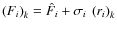 .
.
- 6.
- Estimate the model angular diameter
by minimization for each fabricated data set.
Once the
![]()
![]() minimization procedures are terminated, we can estimate the angular diameter confidence interval from the
minimization procedures are terminated, we can estimate the angular diameter confidence interval from the
![]() distribution thanks to the simple percentile confidence interval method, easy to implement (Efron & Tibshirani 1983): for the
distribution thanks to the simple percentile confidence interval method, easy to implement (Efron & Tibshirani 1983): for the ![]() confidence level, calculate
confidence level, calculate
![]() and
and
![]() ,
the percentiles 100(
,
the percentiles 100(![]() % and 100(
% and 100(
![]() )% relative to the residual-bootstrap distribution of
)% relative to the residual-bootstrap distribution of
![]() ;
then, among all the bootstrap angular diameters with associated
;
then, among all the bootstrap angular diameters with associated
![]() between
between
![]() and
and
![]() ,
find
the smallest and the greatest bootstrap angular diameter estimates
,
find
the smallest and the greatest bootstrap angular diameter estimates
![]() and
and
![]() ,
corresponding to the lower and the upper bounds of the
,
corresponding to the lower and the upper bounds of the
![]() confidence interval.
confidence interval.
Because the mean of the distribution of the
![]() bootstrap
bootstrap
![]() values is not equal to the minimum
values is not equal to the minimum ![]() obtained with the original data set, we instead use the bias corrected percentile confidence interval method (Efron & Tibshirani 1993). In this method, the probabilities
obtained with the original data set, we instead use the bias corrected percentile confidence interval method (Efron & Tibshirani 1993). In this method, the probabilities ![]() and
and
![]() are replaced by
are replaced by
![]() and
and
![]() ,
the values of the standard normal cdf for the points
,
the values of the standard normal cdf for the points
![]() and
and
![]() ,
where p is the proportion of negative
,
where p is the proportion of negative
![]() values, and up is the (100p)th percentile relative to the standard normal cdf.
values, and up is the (100p)th percentile relative to the standard normal cdf.
Formally, if ![]() is the standard normal cdf,
is the standard normal cdf,
![]() ,
,
![]() ,
,
![]() ,
,
![]() ,
and
,
and
![]() .
.
Finally,
![]() and
and
![]() are the smallest and the greatest bootstrap angular diameter estimates with the
are the smallest and the greatest bootstrap angular diameter estimates with the
![]() values between
values between
![]() and
and
![]() .
.
References
- Allende Prieto, C. 2001, ApJ, 547, 200 [NASA ADS] [CrossRef] [Google Scholar]
- Allende Prieto, C., & Lambert, D. L. 2000, AJ, 119, 2445 [NASA ADS] [CrossRef] [Google Scholar]
- Alvarez, R., & Plez, B. 1998, A&A, 330, 1109 [NASA ADS] [Google Scholar]
- Amsler, C., Doser, M., Antonelli, M., et al. 2008, Phys. Lett. B, 667 [Google Scholar]
- Andrews, K. W. 1981, Acta Cryst. Sect. A, 37, 765 [NASA ADS] [CrossRef] [Google Scholar]
- Arenou, F., Grenon, M., & Gomez, A. 1992, A&A, 258, 104 [NASA ADS] [Google Scholar]
- Babu, G. J., & Feigelson, E. D. 1996, Astrostatistics, ed. G. J. Babu, & E. D. Feigelson, Interdisciplinary Statist. Ser. (Chapman - Hall) [Google Scholar]
- Barlow, R. 2003, in Statistical Problems in Particle Physics, Astrophysics and Cosmology, ed. L. Lyons, R. Mount, & R. Reitmeyer, Stanford University (SLAC), 250 [Google Scholar]
- Baschek, B., Scholz, M., & Wehrse, R. 1991, A&A, 246, 374 [NASA ADS] [Google Scholar]
- Beichman, C. A., Neugebauer, G., Habing, H. J., et al. 1988, Infrared astronomical satellite (IRAS) catalogs and atlases, Explanatory supplement, 1 [Google Scholar]
- Bell, R. A., & Gustafsson, B. 1989, MNRAS, 236, 653 [NASA ADS] [CrossRef] [Google Scholar]
- Berdnikov, L. N., & Pavlovskaya, E. D. 1991, SvAL, 17, 215 [NASA ADS] [Google Scholar]
- Bessell, M. S., Castelli, F., & Plez, B. 1998, A&A, 333, 231 [NASA ADS] [Google Scholar]
- Bevington, P. R., & Robinson, D. K. 1992, Data Reduction and Error Analysis for The Physical Sciences, ed. P. R. Bevington, & D. K. Robinson (McGraw-Hill) [Google Scholar]
- Blackwell, D. E., & Shallis, M. J. 1977, MNRAS, 180, 177 [NASA ADS] [CrossRef] [Google Scholar]
- Blackwell, D. E., Petford, A. D., Arribas, S., Haddock, D. J., & Selby, M. J. 1990, A&A, 232, 396 [NASA ADS] [Google Scholar]
- Boden, A. F. 2003, in EAS Public. Ser., ed. G. Perrin, & F. Malbet, 6, 151 [Google Scholar]
- Boden, A. F. 2007, New Astron. Rev., 51, 617 [NASA ADS] [CrossRef] [Google Scholar]
- Bonneau, D., Clausse, J.-M., Delfosse, X., et al. 2006, A&A, 456, 789 [NASA ADS] [CrossRef] [EDP Sciences] [Google Scholar]
- Bordé, P., Coudé du Foresto, V., Chagnon, G., & Perrin, G. 2002, A&A, 393, 183 [NASA ADS] [CrossRef] [EDP Sciences] [Google Scholar]
- Brott, I., & Hauschildt, P. H. 2005, in The Three-Dimensional Universe with Gaia, ed. C. Turon, K. S. O'Flaherty, & M. A. C. Perryman, ESA SP-576, 565 [Google Scholar]
- Brown, A. G. A., Arenou, F., van Leeuwen, F., Lindegren, L., & Luri, X. 1997, in Hipparcos - Venice '97, ESA SP-402, 63 [Google Scholar]
- Buscombe, W. 1962, Mount Stromlo Observatory Mimeographs, 4, 1 [Google Scholar]
- Cardelli, J. A., Clayton, G. C., & Mathis, J. S. 1989, ApJ, 345, 245 [NASA ADS] [CrossRef] [Google Scholar]
- Castelli, F., & Kurucz, R. L. 2003, in Modelling of Stellar Atmospheres, ed. N. Piskunov, W. W. Weiss, & D. F. Gray, IAU Symp., 210, ASP, poster A20 (available on CD-ROM) [Google Scholar]
- Chambers, J. M., Cleveland, W. S., Kleiner, B., & Tukey, P. A. 1983, Graphical methods for data analysis, ed. J. M. Chambers, W. S. Cleveland, B. Kleiner, & P. A. Tukey, The Wadsworth Statist./Probab. Ser. (Duxbury Press) [Google Scholar]
- Chen, B., Vergely, J. L., Valette, B., & Carraro, G. 1998, A&A, 336, 137 [NASA ADS] [Google Scholar]
- Cohen, M., Walker, R. G., Barlow, M. J., & Deacon, J. R. 1992, AJ, 104, 1650 [NASA ADS] [CrossRef] [Google Scholar]
- Cohen, M., Witteborn, F. C., Walker, R. G., Bregman, J. D., & Wooden, D. H. 1995, AJ, 110, 275 [NASA ADS] [CrossRef] [Google Scholar]
- Cohen, M., Witteborn, F. C., Carbon, D. F., et al. 1996, AJ, 112, 2274 [NASA ADS] [CrossRef] [Google Scholar]
- Cohen, M., Walker, R. G., Carter, B., et al. 1999, AJ, 117, 1864 [NASA ADS] [CrossRef] [Google Scholar]
- Cohen, M., Wheaton, W. A., & Megeath, S. T. 2003, AJ, 126, 1090 [NASA ADS] [CrossRef] [Google Scholar]
- Colina, L., Bohlin, R., & F., C. 1996, Absolute Flux Calibrated Spectrum of Vega, Instrument Science Report CAL/SCS-008, STScI [Google Scholar]
- Cruzalèbes, P., Spang, A., & Sacuto, S. 2008, in The 2007 ESO Instrument Calibration Workshop, ed. A. Kaufer, & F. Kerber, ESO (Springer), 479 [Google Scholar]
- Cutri, R. M., Skrutskie, M. F., van Dyk, S., et al. 2003, 2MASS All Sky Catalog of point sources (NASA/IPAC) [Google Scholar]
- D'Agostini, G., & Raso, M. 2000, arXiv High Energy Physics, Experiment e-prints [Google Scholar]
- de Graauw, T., Haser, L. N., Beintema, D. A., et al. 1996, A&A, 315, L49 [NASA ADS] [Google Scholar]
- de Jager, C., & Nieuwenhuijzen, H. 1987, A&A, 177, 217 [NASA ADS] [Google Scholar]
- Decin, L., & Eriksson, K. 2007, A&A, 472, 1041 [NASA ADS] [CrossRef] [EDP Sciences] [Google Scholar]
- Decin, L., Waelkens, C., Eriksson, K., et al. 2000, A&A, 364, 137 [NASA ADS] [Google Scholar]
- Decin, L., Shkedy, Z., Molenberghs, G., Aerts, M., & Aerts, C. 2004, A&A, 421, 281 [NASA ADS] [CrossRef] [EDP Sciences] [Google Scholar]
- Delfosse, X. 2004, Stellar diameter estimation from photospheric indices, Tech. rep., JMMC [Google Scholar]
- di Benedetto, G. P. 1993, A&A, 279, 315 [NASA ADS] [Google Scholar]
- di Benedetto, G. P. 1998, A&A, 339, 858 [NASA ADS] [Google Scholar]
- Di Folco, E., Thévenin, F., Kervella, P., et al. 2004, A&A, 426, 601 [NASA ADS] [CrossRef] [EDP Sciences] [Google Scholar]
- Dogan, G. 2007, System Dynamics Rev., 23, 415 [CrossRef] [Google Scholar]
- Dommanget, J., & Nys, O. 2002, VizieR Online Data Catalog, 1274, 0 [Google Scholar]
- Drimmel, R., & Spergel, D. N. 2001, ApJ, 556, 181 [NASA ADS] [CrossRef] [Google Scholar]
- Efron, B. 1979, Ann. Statist., 7, 1 [CrossRef] [MathSciNet] [Google Scholar]
- Efron, B. 1982, The Jacknife, the Bootstrap, and other Resampling Plans, ed. B. Efron, Reg. Conf. Ser. in Applied Math., 38 (SIAM-NF-CBMS) [Google Scholar]
- Efron, B., & Tibshirani, R. 1983, Statist. Sci., 1, 54 [Google Scholar]
- Efron, B., & Tibshirani, R. 1993, Monographs and Statist. and Applied Probab., An Introduction to the Bootstrap, ed. B. Efron, & R. Tibshirani (Chapman - Hall/CRC), 57 [Google Scholar]
- Engelke, C. W. 1992, AJ, 104, 1248 [NASA ADS] [CrossRef] [Google Scholar]
- Fiorucci, M., & Munari, U. 2003, A&A, 401, 781 [NASA ADS] [CrossRef] [EDP Sciences] [Google Scholar]
- Fitzgerald, M. P. 1968, AJ, 73, 983 [NASA ADS] [CrossRef] [Google Scholar]
- Fitzpatrick, E. L. 1999, PASP, 111, 63 [NASA ADS] [CrossRef] [Google Scholar]
- Fracassini, M., Pasinetti, L. E., & Manzolini, F. 1981, A&AS, 45, 145 [NASA ADS] [Google Scholar]
- Friedmann, D. A. 1981, Ann. Statist., 9, 1218 [Google Scholar]
- Goodman, J. W. 1985, Statistical Optics, ed. J. W. Goodman (Wiley Classics Libr.) [Google Scholar]
- Gray, D. F. 2005, The Observation and Analysis of Stellar Photospheres, 3rd edn. (Cambridge Univ. Press) [Google Scholar]
- Groenewegen, M. A. T. 2004, MNRAS, 353, 903 [NASA ADS] [CrossRef] [Google Scholar]
- Gustafsson, B., Bell, R. A., Eriksson, K., & Nordlund, A. 1975, A&A, 42, 407 [NASA ADS] [Google Scholar]
- Gustafsson, B., Edvardsson, B., Eriksson, K., et al. 2003, in Stellar Atmosphere Modeling, ed. I. Hubeny, D. Mihalas, & K. Werner, ASP Conf. Ser., 288, 331 [Google Scholar]
- Gustafsson, B., Edvardsson, B., Eriksson, K., et al. 2008, A&A, 486, 951 [NASA ADS] [CrossRef] [EDP Sciences] [Google Scholar]
- Hakkila, J., Myers, J. M., Stidham, B. J., & Hartmann, D. H. 1997, AJ, 114, 2043 [NASA ADS] [CrossRef] [Google Scholar]
- Hauschildt, P. H. 1992, J. Quant. Spec. Radiat. Transf., 47, 433 [Google Scholar]
- Heras, A. M., Shipman, R. F., Price, S. D., et al. 2002, A&A, 394, 539 [NASA ADS] [CrossRef] [EDP Sciences] [Google Scholar]
- Houk, N. 1978, Michigan catalogue of two-dimensional spectral types for the HD stars, ed. N. Houk [Google Scholar]
- Jancart, S., Jorissen, A., Babusiaux, C., & Pourbaix, D. 2005, A&A, 442, 365 [NASA ADS] [CrossRef] [EDP Sciences] [Google Scholar]
- JCGM/WG 1 2008, Evaluation of measurement data - Guide to the expression of uncertainty in measurement (JCGM 100:2008, GUM 1995 with minor corrections) [Google Scholar]
- Johnson, H. L. 1966, ARA&A, 4, 193 [NASA ADS] [CrossRef] [Google Scholar]
- Kelley, K. 2007, J. Statist. Soft., 20, 1 [Google Scholar]
- Kervella, P., Nardetto, N., Bersier, D., Mourard, D., & Coudé du Foresto, V. 2004, A&A, 416, 941 [NASA ADS] [CrossRef] [EDP Sciences] [Google Scholar]
- Kotz, S., & Van Dorp, J. 2004, Beyond beta: other continuous families of distributions with bounded support, ed. S. Kotz, & J. Van Dorp (Word Scien. Pub.) [Google Scholar]
- Kovalevsky, J., & Seidelmann, P. K. 2004, Fundamentals of Astrometry, ed. J. Kovalevsky, & P. K. Seidelmann (Cambridge Univ. Press) [Google Scholar]
- Kurucz, R. L. 1979, ApJS, 40, 1 [NASA ADS] [CrossRef] [Google Scholar]
- Kucinskas, A., Hauschildt, P. H., Ludwig, H.-G., et al. 2005, A&A, 442, 281 [NASA ADS] [CrossRef] [EDP Sciences] [Google Scholar]
- Leech, K., Kester, D., Shipman, R., et al. 2003, The ISO Handbook, Volume V, SWS, The Short Wavelength Spectrometer [Google Scholar]
- Levenberg, K. 1944, Quart. Appl. Math., 2, 164 [Google Scholar]
- Lorente, R. 1998, Spectral resolution of SWS AOT 1, IDC Internal Report, ISO Data Centre [Google Scholar]
- Luri, X., & Arenou, F. 1997, in ESA Special Publication, Hipparcos - Venice '97, 402, 449 [Google Scholar]
- Malacara, D., & Thompson, B. J. 2001, Handbook of optical engineering, ed. D. Malacara, & B. J. Thompson (CRC Press) [Google Scholar]
- Marengo, M. 2000, Ph.D. Thesis, Internat. School for Adv. Studies (SISSA/ISAS), Harvard-Smithsonian Center for Astrophysics [Google Scholar]
- Marquardt, D. 1963, SIAM J. Appl. Math., 11, 431 [Google Scholar]
- Meisner, J. 2008, in The Power of Optical/IR Interferometry: Recent Scientific Results and 2nd Generation, ed. A. Richichi, F. Delplancke, F. Paresce, & A. Chelli, 481 [Google Scholar]
- Meléndez, J., Asplund, M., Alves-Brito, A., et al. 2008, A&A, 484, L21 [NASA ADS] [CrossRef] [EDP Sciences] [MathSciNet] [Google Scholar]
- Mérand, A., Bordé, P., & Coudé Du Foresto, V. 2005, A&A, 433, 1155 [NASA ADS] [CrossRef] [EDP Sciences] [Google Scholar]
- Millour, F., Petrov, R., Malbet, F., et al. 2008, in The 2007 ESO Instrument Calibration Workshop, ed. A. Kaufer, & F. Kerber, ESO (Springer), 461 [Google Scholar]
- Morel, M., & Magnenat, P. 1978, A&AS, 34, 477 [NASA ADS] [Google Scholar]
- Mozurkewich, D., Johnston, K. J., Simon, R. S., et al. 1991, AJ, 101, 2207 [NASA ADS] [CrossRef] [Google Scholar]
- Nagy, T. A., & Hill, R. S. 1980, Documentation for the machine-readable version of the UBVRIJKLMNH photoelectric photometric catalogue, Tech. rep., NASA [Google Scholar]
- NASA Exoplanet Science Institute 2008, The getCal Interferometric Observation Planning Tool Suite, 2.10.7 edn., Cal. Inst. Tech. [Google Scholar]
- Neckel, T., & Klare, G. 1980, A&AS, 42, 251 [Google Scholar]
- Palm, R. 2002, Biotechnol. Agron. Soc. Environ., 6, 143 [Google Scholar]
- Pasinetti Fracassini, L. E., Pastori, L., Covino, S., & Pozzi, A. 2001, A&A, 367, 521 [NASA ADS] [CrossRef] [EDP Sciences] [Google Scholar]
- Penprase, B. E. 1992, ApJS, 83, 273 [NASA ADS] [CrossRef] [Google Scholar]
- Perryman, M. A. C., Lindegren, L., Kovalevsky, J., et al. 1997, A&A, 323, L49 [NASA ADS] [Google Scholar]
- Petrov, R. G., Malbet, F., Weigelt, G., et al. 2007, A&A, 464, 1 [NASA ADS] [CrossRef] [EDP Sciences] [Google Scholar]
- Pickles, A. J. 1998, PASP, 110, 863 [CrossRef] [Google Scholar]
- Prasad, C. D. 1998, Bull. Astr. Soc. Ind., 26, 253 [NASA ADS] [Google Scholar]
- Press, W. H., Teukolsky, S. A., Vetterling, W. T., & Flannery, B. P. 2007, Numerical Recipes 3rd edn, The Art of Scientific Computing, ed. W. H. Press, S. A. Teukolsky, W. T. Vetterling, & B. P. Flannery (Cambridge Univ. Press) [Google Scholar]
- Richichi, A., & Percheron, I. 2002, A&A, 386, 492 [NASA ADS] [CrossRef] [EDP Sciences] [Google Scholar]
- Richichi, A., Percheron, I., & Khristoforova, M. 2005, A&A, 431, 773 [NASA ADS] [CrossRef] [EDP Sciences] [Google Scholar]
- Richichi, A., Percheron, I., & Davis, J. 2009, MNRAS, 399, 399 [NASA ADS] [CrossRef] [Google Scholar]
- Sacuto, S., Jorissen, A., Cruzalèbes, P., et al. 2008, A&A, 482, 561 [NASA ADS] [CrossRef] [EDP Sciences] [Google Scholar]
- Seaton, M. J. 1979, MNRAS, 187, 785 [NASA ADS] [Google Scholar]
- Skrutskie, M. F., Cutri, R. M., Stiening, R., et al. 2006, AJ, 131, 1163 [NASA ADS] [CrossRef] [Google Scholar]
- Sloan, G. C., Kraemer, K. E., Price, S. D., & Shipman, R. F. 2003, ApJS, 147, 379 [NASA ADS] [CrossRef] [Google Scholar]
- Smalley, B. 2005, Mem. Soc. Astron. It. Suppl., 8, 130 [Google Scholar]
- Smithson, M. J. 2002, Confidence Intervals, ed. M. J. Smithson, Quantit. Appl. in Soc. Scien. Ser., 07-140 (SAGE Univ. Papers) [Google Scholar]
- Straizys, V., & Kuriliene, G. 1981, Ap&SS, 80, 353 [NASA ADS] [CrossRef] [Google Scholar]
- Tatulli, E., Millour, F., Chelli, A., et al. 2007, A&A, 464, 29 [NASA ADS] [CrossRef] [EDP Sciences] [Google Scholar]
- van Belle, G. T. 1999, PASP, 111, 1515 [NASA ADS] [CrossRef] [Google Scholar]
- van Belle, G. T., & van Belle, G. 2005, PASP, 117, 1263 [NASA ADS] [CrossRef] [Google Scholar]
- van Belle, G. T., Lane, B. F., Thompson, R. R., et al. 1999, AJ, 117, 521 [NASA ADS] [CrossRef] [Google Scholar]
- van Belle, G. T., van Belle, G., Creech-Eakman, M. J., et al. 2008, ApJS, 176, 276 [NASA ADS] [CrossRef] [Google Scholar]
- Verhoelst, T. 2005, Ph.D. Thesis, Institute of Astronomy, K.U. Leuven, Belgium [Google Scholar]
- Volk, K., & Cohen, M. 1989, AJ, 98, 1918 [NASA ADS] [CrossRef] [Google Scholar]
- Williams, D. A. 1992, The Astronomy and Astrophysics Encyclopedia, ed. D. A. Williams (Cambridge Univ. Press), 350 [Google Scholar]
- Winzer, P. 2000, Rev. Sci. Instrum., 71, 1447 [NASA ADS] [CrossRef] [Google Scholar]
- Wittkowski, M., Aufdenberg, J. P., & Kervella, P. 2004, A&A, 413, 711 [NASA ADS] [CrossRef] [EDP Sciences] [Google Scholar]
- Wittkowski, M., Hummel, C. A., Aufdenberg, J. P., & Roccatagliata, V. 2006, A&A, 460, 843 [NASA ADS] [CrossRef] [EDP Sciences] [Google Scholar]
- Zhang, Y., Luo, A., & Zhao, Y. 2004, in Data Processing Systems: Hardware and Algorithms, ed. P. J. Queen, & A. Bridger, Proc. SPIE, 5493, 521 [Google Scholar]
Footnotes
- ... database
- simbad.u-strasbg.fr/simbad/
- ... JMMC-SearchCal
- www.jmmc.fr/searchcal_page.htm
- ... MSC-getCal
- nexsciweb.ipac.caltech.edu/gcWeb/gcWeb.jsp
- ... ESO-CalVin
- www.eso.org/observing/etc/
- ... 2MASS catalogue
- www.ipac.caltech.edu/2mass/
- ... ISO-SWS
- irsa.ipac.caltech.edu/data/SWS/
- ... IRAS-LRS
- www.iras.ucalgary.ca/satellites/Iras/getlrs.html
- ... LBSI
- cdsarc.u-strasbg.fr/viz-bin/Cat?J/A+A/393/183
- ... MCC
- ster.kuleuven.ac.be/~tijl/MIDI_calibration/mcc.txt
- ... page
- www.am.ub.es/~carrasco/models/synthetic.html
- ... models
- kurucz.harvard.edu/
- ... code
- www.hs.uni-hamburg.de/EN/For/ThA/phoenix/
- ... models
- marcs.astro.uu.se/
- ... Systems
- ulisse.pd.astro.it/Astro/ADPS/
- ... online
- nexsciweb.ipac.caltech.edu/gcWeb/doc/getCal/ gcManual.html
- ... observations
- ESO programme ID 080.D-0076A (AMBER GTO).
- ...
SPIDAST
- SPectro-Interferometric Data Analysis Software Tool.
- ... NIST/SEMATECH
- www.itl.nist.gov/div898/handbook/
All Tables
Table 1:
Values of the angular diameter ![]() (in mas), under which
(in mas), under which
![]() ,
at
,
at
![]() .
.
Table 2:
Broadband photometry of ![]() Gru and reddening.
Gru and reddening.
Table 3:
Effective wavelength and bandwidth (in square brackets) in each band (both in ![]() m), for a K2 spectral type spectrum and a [4250] K blackbody spectrum.
m), for a K2 spectral type spectrum and a [4250] K blackbody spectrum.
Table 4: Photometric angular diameters (in mas) obtained with various synthetic spectra (with T = [4250] K) in the 2MASS near-infrared bands.
Table 5: Angular diameters obtained by fitting various models (with T = [4250] K) to visible and/or NIR photometric data.
Table 6: Spectral characteristics of the SWS AOT-1 bands and their photometric accuracy.
Table 7:
Angular diameters obtained by fitting various models (with T = [4250] K) to the 2.38-[27.5] ![]() m SWS spectrum.
m SWS spectrum.
Table 8:
Fundamental parameter estimates (with uncertainties) of ![]() Gru reevaluated from our study.
Gru reevaluated from our study.
Table B.1:
Total visual extinction of ![]() Gru as obtained from the relevant studies.
Gru as obtained from the relevant studies.
All Figures
|
|
Figure 1:
Left panel: plot of the uniform-disk visibility function against the argument
|
| Open with DEXTER | |
| In the text | |
|
|
Figure 2:
Log-log plot of the angular diameter |
| Open with DEXTER | |
| In the text | |
|
|
Figure 3:
Log-log plot of the broadband absolute photometry (in
|
| Open with DEXTER | |
| In the text | |
|
|
Figure 4:
Log-log plot of the high-resolution processed SWS01 spectrum (in
|
| Open with DEXTER | |
| In the text | |
|
|
Figure 5:
High-resolution (R=20 000) MARCS synthetic spectral radiant exitance (in
|
| Open with DEXTER | |
| In the text | |
|
|
Figure 6:
Median-resolution (R=1000) TURBOSPECTRUM synthetic radiance data,
obtained with the same model parameters as for Fig. 5. Upper left panel: spectral distribution of the central radiance. Upper right panel: spectral distribution of the radiance normalized to the centre, for r=0.345 (upper curve), 0.515, 0.631, 0.720, 0.791, 0.848, 0.883, 0.922, 0.952, 0.974, 0.990, and 0.998 (lower curve). Lower left panel: normalized radiance profiles, for the wavelengths
|
| Open with DEXTER | |
| In the text | |
|
|
Figure 7:
Plot of |
| Open with DEXTER | |
| In the text | |
|
|
Figure 8: Histogram of the angular diameters estimated by residual bootstrapping when fitting the MARCS model on the SWS spectrum. |
| Open with DEXTER | |
| In the text | |
|
|
Figure 9:
Estimated sizes of |
| Open with DEXTER | |
| In the text | |
|
|
Figure C.1: Left panel: plot of the spectral distribution of the original centred Pearson residuals, obtained by fitting the MARCS model on the SWS spectrum. The residual values located above and below the two horizontal dashed lines are identified as extreme outliers. Right panel: histogram of the Pearson residual distribution. The thin curve within the histogram is the normal probability density function shown for comparison. The two vertical dashed lines give the positions of the upper and lower outer fences identifying the extreme outliers. |
| Open with DEXTER | |
| In the text | |
| |
Figure C.2:
Left panel: cumulative histogram of the
|
| Open with DEXTER | |
| In the text | |
Copyright ESO 2010
Current usage metrics show cumulative count of Article Views (full-text article views including HTML views, PDF and ePub downloads, according to the available data) and Abstracts Views on Vision4Press platform.
Data correspond to usage on the plateform after 2015. The current usage metrics is available 48-96 hours after online publication and is updated daily on week days.
Initial download of the metrics may take a while.