| Issue |
A&A
Volume 515, June 2010
|
|
|---|---|---|
| Article Number | A15 | |
| Number of page(s) | 9 | |
| Section | Astrophysical processes | |
| DOI | https://doi.org/10.1051/0004-6361/200913678 | |
| Published online | 31 May 2010 | |
Kerr geodesics, the Penrose process and jet collimation by a black hole
J. Gariel1 - M. A. H. MacCallum2 - G. Marcilhacy1 - N. O. Santos1,2,3
1 - LERMA-UPMC, Université Pierre et Marie Curie,
Observatoire de Paris, CNRS, UMR 8112, 3 rue Galilée, 94200
Ivry-sur-Seine, France
2 -
School of Mathematical Sciences,
Queen Mary, University of London,
Mile End Road, London E1 4NS, UK
3 -
Laboratório Nacional de Computação Científica,
25651-070 Petrópolis RJ, Brazil
Received 16 November 2009 / Accepted 10 February 2010
Abstract
Aims. We re-examine the possibility that astrophysical jet
collimation may arise from the geometry of rotating black holes and the
presence of high-energy particles resulting from a Penrose process,
without the help of magnetic fields.
Methods. Our analysis uses the Weyl coordinates, which are
revealed better adapted to the desired shape of the jets. We
numerically integrate the 2D-geodesics equations.
Results. We give a detailed study of these geodesics and give
several numerical examples. Among them are a set of perfectly
collimated geodesics with asymptotes
![]() parallel to the z-axis, with
parallel to the z-axis, with ![]() only depending on the ratios
only depending on the ratios
![]() and
and
![]() ,
where a and M are the parameters of the Kerr black hole, E the particle energy and
,
where a and M are the parameters of the Kerr black hole, E the particle energy and
![]() the Carter's constant.
the Carter's constant.
Key words: black hole physics - acceleration of particules - relativistic processes
1 Introduction
It has long been speculated that a single mechanism might be at work in the production and collimation of various very energetic observed jets, such as those in gamma ray bursts (GRB, Fargion 2003; Sheth et al. 2003; Piran et al. 2001), and jets ejected from active galactic nuclei (AGN) (Sauty et al. 2002) and from microquasars (Mirabel & Rodriguez 1999,1994). Here we limit ourselves to jets produced by a black hole (BH) type core. The most often invoked process is the Blandford-Znajek (Blandford & Znajek 1977) or some closely similar mechanism (e.g. Punsly & Coroniti 1990a,b; Punsly 2001) in the framework of magnetohydrodynamics, always requiring a magnetic field. However such mechanisms are limited to charged particles, and would be inefficient for neutral particles (neutrons, neutrinos and photons), which are currently the presumed antecedents of very thin and long duration GRB (Fargion 2003). Moreover, even for charged particles, some questions persist (see for instance the conclusion of Williams 2004). Finally, while the observations of synchrotron radiation prove the presence of magnetic fields, they do not prove that those fields alone cause the collimation: magnetic mechanisms may be only a part of a more unified mechanism for explaining the origin and collimation of powerful jets (see Livio 1999, p. 234, and Sect. 5), and, in particular, for collimation of jets from AGN to subparsec scales (see de Felice & Zanotti 2000).
Considering this background, it is worthwhile looking for other types of model to explain the origin and structure of jets. Other models based on a purely general relativistic origin for jets have been considered. A simple model was obtained by Opher et al. (1996) by assuming the centres of galaxies are described by a cylindrical rotating dust. That paper showed that confinement occurs in the radial motion of test particles while the particles are accelerated in the axial direction thus producing jets. Another relativistic model was put forward in Herrera & Santos (2007). This showed that the sign of the proper acceleration of test particles near the axis of symmetry of quasi-spherical objects and close to the horizon can change. Such an outward acceleration, that can be very big, might cause the production of jets.
However, these models show a powerful gravitational effect of repulsion only near the axis, and are built in the framework of axisymmetric stationary metrics which do not have an asymptotic behaviour compatible with possible far away observations. So we want to explore the more realistic rotating black hole, i.e. Kerr, metrics instead.
We thus address here the issue of whether it is possible, at least in principle (i.e. theoretically) to obtain a very energetic and perfectly collimated jet in a Kerr black hole spacetime without making use of magnetic fields. Other authors (see Williams 1995; de Felice & Carlotto 1997; Bicák et al. 1993; Williams 2004, and references therein) have made related studies to which we refer below. Most such authors agree that the strong gravitational field generated by rotating BHs is essential to understanding the origin of jets, or more precisely that the jet originates from a Penrose-like process (Penrose 1969; Williams 2004) in the ergosphere of the BH; collimation may also arise from the gravitational field and that is the main topic in this paper.
Our work can therefore be considered as covering the whole class of models in which particles coming from the ergosphere form a jet collimated by the geometry. Although a complete model of an individual jet would require use of detailed models of particle interactions inside the ergosphere, such as that given by Williams (2004), we show that thin and very long and energetic jets, with some generic features, can be produced in this way. In particular the presence of a characteristic radius, of the size of the ergosphere, around which one would find the most energetic particles, might be observationally testable.
From a strictly general relativistic point of view, test particles in vacuum (here, a Kerr spacetime) follow geodesics; this applies to both charged and uncharged particles, although, of course, in an electrovacuum spacetime, such as Kerr-Newman, charged particles would follow accelerated trajectories, not geodesics. Thus, in Kerr fields, what produces an eventual collimation for test particles, or not, is the form of the resulting geodesics. Hence we discuss here the possibilities of forming an outgoing jet of collimated geodesics followed by particles arising from a Penrose-like process inside the ergosphere of a Kerr BH. We show that it is possible in principle to obtain such a jet from a purely gravitational model, but it would require the ``Penrose process'' to produce a suitable, and rather special, distribution of outgoing particles.
The model is based on the following considerations.
Most studies of geodesics, (e.g. Chandrasekhar 1983), employ generalized spherical, i.e. Boyer-Lindquist, coordinates. We transform to Weyl coordinates, which are generalized cylindrical coordinates, and are more appropriate, as we shall see, for interpreting the collimated jets.
We consider test particles moving in the axisymmetric stationary gravitational field produced by the Kerr spacetime, whose geodesic equations, as projected into a meridional plane, are known (Chandrasekhar 1983). Our study is restricted to massive test particles, moving on timelike geodesics, but of course massless test particles on null geodesics could be the subject of a similar study (Incidentally the compendium of Sharp 1979 shows that analytic studies of general timelike geodesics have been much less frequent than detailed studies of more restricted problems).
For particles outgoing from the ergosphere of the Kerr BH we examine their asymptotic behaviour. Among the geodesic particles incoming to the ergosphere, we discuss only the ones coming from infinity parallel to the equatorial plane, because these are in practice the particles stemming from the accretion disk. We show that only those with a small impact parameter are of high enough energy to provide energetic outgoing particles.
In the ergosphere, a Penrose-like process can occur. In the original Penrose
process, an incoming particle decays into two parts inside the ergosphere.
It could also decay into more than two parts, or undergo a collision with
another particle in this region, or give rise to pair creation
![]() from incident photons which would follow null geodesics. The
different possible cases do not affect our considerations, and that is why
we do not study them here, although the distribution function of outgoing
particles would be required in a more detailed model of the type discussed,
in particular to explain why only particles with low angular momentum and
not diverging from the rotation axis are produced. For detailed studies see
Williams (1995,2004) and Piran & Shaham (1977). After a decay, one (or more) of the particles
produced crosses the event horizon and irreversibly plunges into the BH,
while a second particle arising from the decay can be ejected out of the
ergosphere following a geodesic towards infinity. This outgoing particle
could be ejected so that asymptotically it runs parallel to the axis of
symmetry, but we do not discuss only such particles.
from incident photons which would follow null geodesics. The
different possible cases do not affect our considerations, and that is why
we do not study them here, although the distribution function of outgoing
particles would be required in a more detailed model of the type discussed,
in particular to explain why only particles with low angular momentum and
not diverging from the rotation axis are produced. For detailed studies see
Williams (1995,2004) and Piran & Shaham (1977). After a decay, one (or more) of the particles
produced crosses the event horizon and irreversibly plunges into the BH,
while a second particle arising from the decay can be ejected out of the
ergosphere following a geodesic towards infinity. This outgoing particle
could be ejected so that asymptotically it runs parallel to the axis of
symmetry, but we do not discuss only such particles.
In our model there is no appeal to electromagnetic forces to explain the ejection or the collimation of jets, though the particles therein may themselves be charged. The gravitational field suffices, in the case of strong fields in general relativity, which is the case near the Kerr BH, provided the ergosphere produces particles of appropriate energy and initial velocity. The gravitomagnetic part of the gravitational field then provides the collimation. Hence, our model is, in this respect, simpler than the standard model of Blandford & Znajek (1977), and is in accordance with the analysis given in Williams (2004).
The paper starts with a study of Kerr geodesics in Weyl coordinates in Sect. 2; the next section studies the asymptotic behaviour of geodesics of outgoing particles with Lz=0; Sect. 4 analyses incoming particles stemming from the accretion; a sample Penrose process and the plotting of geodesics are presented in Sect. 5; and finally we discuss in Sect. 6 the significance of our results for jets. In the conclusion, we succinctly summarize our main results and evoke some perspectives.
2 Kerr geodesics
We start from the projection in a meridional plane
![]() of the
Kerr geodesics in Boyer-Lindquist spherical coordinates
of the
Kerr geodesics in Boyer-Lindquist spherical coordinates ![]() ,
,
![]() and
and ![]() .
The metric is
.
The metric is
where M and Ma are, respectively, the mass and the angular momentum of the source, and we have taken units such that c=1=G where G is Newton's constant of gravitation. The ``radial'' coordinate in Eq. (1) has been named
![$\displaystyle \frac{(a_4r^4+a_3r^3+a_2r^2+a_1r+a_0)}{ \left[r^2+\left(\frac{a}{M}\right)^2\cos^2\theta\right]^{2}},$](/articles/aa/full_html/2010/07/aa13678-09/img34.png)
![$\displaystyle \frac{b_4\cos^4\theta+b_2\cos^2\theta+b_0}{(1-\cos^2\theta) \left[r^2+\left(\frac{a}{M}\right)^2\cos^2\theta\right]^{2}},$](/articles/aa/full_html/2010/07/aa13678-09/img36.png)
with coefficients
and
where the dot stands for differentiation with respect to an affine parameter and E, Lz and
The dimensionless Weyl cylindrical coordinates, in multiples of geometrical
units of mass M, are given by
![\begin{displaymath}\rho =\left[ (r-1)^{2}-A\right] ^{1/2}\sin \theta ,\;\;z=(r-1)\cos \theta ,
\end{displaymath}](/articles/aa/full_html/2010/07/aa13678-09/img47.png)
where

From (12) we have the inverse transformation
with
![\begin{displaymath}\alpha =\frac{1}{2}\left( \left[\rho ^{2}+(z+\sqrt{A})^{2}\right]^{1/2}+\left[\rho ^{2}+(z-\sqrt{A})^{2}\right]^{1/2} \right).
\end{displaymath}](/articles/aa/full_html/2010/07/aa13678-09/img52.png)
Here we have assumed
The Eq. (16) shows that in the ![]() plane the curves of
constant
plane the curves of
constant ![]() (constant r) are ellipses with semi-major axis
(constant r) are ellipses with semi-major axis ![]() and eccentricity
and eccentricity
![]() :
for large
:
for large ![]() ,
these approximate
circles. Note that
,
these approximate
circles. Note that ![]() consists of the rotation axis
consists of the rotation axis ![]() or
or ![]() together with the ergosphere surface.
together with the ergosphere surface.
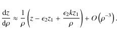
Now, with Eqs. (14) and (15) we can write the geodesics Eqs. (2)
and (3) in terms of ![]() and z coordinates, producing the
following autonomous system of first order equations
and z coordinates, producing the
following autonomous system of first order equations
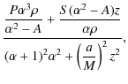
![$\displaystyle (Pz-S)\alpha \left[ (\alpha +1)^{2}\alpha ^{2}+\left( \frac{a}{M}
\right) ^{2}z^{2}\right] ^{-1},$](/articles/aa/full_html/2010/07/aa13678-09/img66.png)
where
and
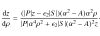
The ratio between the first order differential Eqs. (17) and (18) yields the special characteristic equation of this system of equations
We restrict our study to the quadrant
Geodesics going to or coming from the expected accretion disk would, if the
disk were thin, go to or from values of ![]() much larger than z. In this
limit (
much larger than z. In this
limit (
![]() and
and
![]() ), we have
), we have
| (22) | |||
| (23) | |||
|
(24) | ||
| (25) |
and thus
where
and we have to assume
The truncated series development of
![]() now
yields
now
yields
If
A thicker accretion disk would absorb or release particles on geodesics with
larger values of ![]() ,
which might include particles with
,
which might include particles with
![]() .
.
Geodesics in an axial jet would have ![]() .
For this limit, we first
observe that from Eq. (20) we have
.
For this limit, we first
observe that from Eq. (20) we have
![\begin{displaymath}S\approx \epsilon _{2}\left[ (b_{0}+b_{2}+b_{4})z^{4}+(2b_{0}+b_{2})\rho
^{2}z^{2}\right] ^{1/2}+O(z^{-1}),
\end{displaymath}](/articles/aa/full_html/2010/07/aa13678-09/img93.png)
where

Hence in this limit S is well defined and real for indefinitely small
Before doing so, we may note that in contrast to geodesics with
![]() ,
geodesics with E2>1 and Lz=0 may lie arbitrarily close to the polar
axis (Carter 1968). For
,
geodesics with E2>1 and Lz=0 may lie arbitrarily close to the polar
axis (Carter 1968). For
![]() ,
the value of S2 at the axis is
-z2Lz2 <0 which is not allowed and thus there is some upper bound
,
the value of S2 at the axis is
-z2Lz2 <0 which is not allowed and thus there is some upper bound ![]() on
on ![]() .
The value of S2 at
.
The value of S2 at
![]() is
is
![]() so if
so if
![]() there is also a lower bound
there is also a lower bound ![]() on
on ![]() .
.
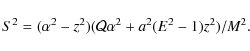
3 Geodesics with

We shall discuss unbounded (E2>1) outgoing geodesics. Corresponding
incoming geodesics will follow the same curves in the opposite direction.
For Lz=0, S2 factorizes as
Hence S can only be zero at the symmetry axis, where
Thus for Lz=0 and
![]() ,
geodesics which initially have
,
geodesics which initially have
![]() will become asymptotic to
will become asymptotic to
![]() .
The angle may be narrow if
.
The angle may be narrow if
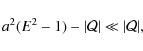
and then
Our other polynomial, P2, can be written as
From this form it easily follows that any unbound geodesic (E2>1) with Lz=0 has at most one turning point in r (i.e. value such that
Although there are no turning points of r, one can have turning points of ![]() ,
if
,
if
![]() .
Such turning points are solutions of the equation
.
Such turning points are solutions of the equation
where
For outgoing geodesics outside (35) which reach points at large zand ![]() (
(
![]() ), then unless the ratio of z to
), then unless the ratio of z to ![]() is very
large (the case which we discuss next) or very small, approximating Eq. (21) gives
is very
large (the case which we discuss next) or very small, approximating Eq. (21) gives
![]() ,
so all such
geodesics approximate
,
so all such
geodesics approximate ![]() for suitable C, regardless of the sign of
for suitable C, regardless of the sign of
![]() .
.
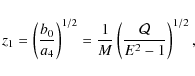
In the limit ![]() and
and
![]() ,
,
| |
= | z(1+O(z -2)), | (36) |
| |P| | = | (37) | |
| |S| | = | (38) |
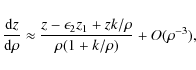
so the Eq. (21) can be approximated by
where
![$\displaystyle \left( \frac{2b_{0}+b_{2}}{a_{4}}\right) ^{1/2}=\rho_{\rm e}\left[
1+\frac{\mathcal{Q}}{a^{2}(E^{2}-1)}\right] ^{1/2},$](/articles/aa/full_html/2010/07/aa13678-09/img137.png)
and
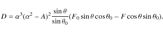
In Fig. 1 we show a plot of the values of
![]() ,
using (21), for
,
using (21), for
![]() ,
with the
parameters M=1, a=1/2, E=104,
,
with the
parameters M=1, a=1/2, E=104,
![]() .
The
only asymptotes are parallel to the z axis at
.
The
only asymptotes are parallel to the z axis at
![]() as
expected from Eq. (40).
as
expected from Eq. (40).
![\begin{figure}
\par\includegraphics[width=8cm,clip]{AA-2009-13678-fig1.eps}
\end{figure}](/articles/aa/full_html/2010/07/aa13678-09/img146.png)
|
Figure 1:
Plot of the surface
|
| Open with DEXTER | |
We also plot in Fig. 2 a set of such outgoing geodesics obeying (21), for the same values of the parameters of the BH (a=1/2, M=1)
and of the particle (Lz=0,
![]() ,
,
![]() ,
so
,
so
![]() ), but with different initial values of the position.
The set of turning points of these geodesics is the curve defined by
Eq. (35). For the rightmost of these geodesics, the numerical
integration was also continued back towards the ergosphere as far as
), but with different initial values of the position.
The set of turning points of these geodesics is the curve defined by
Eq. (35). For the rightmost of these geodesics, the numerical
integration was also continued back towards the ergosphere as far as
![]() ,
,
![]() .
.
![\begin{figure}
\par\includegraphics[width=6cm,height=6cm,clip]{AA-2009-13678-fig2.eps}
\end{figure}](/articles/aa/full_html/2010/07/aa13678-09/img153.png)
|
Figure 2:
Plots of geodesics obeying Eq. (21), showing
the turning points. From left to right these curves start at
|
| Open with DEXTER | |
To confirm the picture obtained from these numerical experiments, one can
show, without assuming
![]() ,
the existence of exactly one zero of Don any curve r= constant,
,
the existence of exactly one zero of Don any curve r= constant,
![]() ,
so that the conclusion that a
geodesic has at most one turning point in
,
so that the conclusion that a
geodesic has at most one turning point in ![]() is not an artefact of the
approximation at large z. The argument is as follows.
is not an artefact of the
approximation at large z. The argument is as follows.
Along an r= constant curve, |P| and ![]() are constant,
are constant,
![]() and
and
![]() ,
where
,
where ![]() is a
constant (related to r). Then
is a
constant (related to r). Then
| D | = | (41) |
where, defining
| F | |||
| = | (42) |
from Eq. (32) we have
At
![]() ,
D>0, while at small
,
D>0, while at small ![]() ,
D<0. Hence there is
at least one zero of D. Let the largest one be at
,
D<0. Hence there is
at least one zero of D. Let the largest one be at
![]() say.
On the r= constant curve, we will then have
say.
On the r= constant curve, we will then have
|
(43) |
Here we have used D=0 at
For large z we see from Eq. (39) that the turning points lie
approximately on a curve
![]() or
or
![]() .
Actually, the differential equation for large z, if we drop the 1/z2terms, has an analytic solution
.
Actually, the differential equation for large z, if we drop the 1/z2terms, has an analytic solution
where C is a constant of integration, so
as
From Eq. (45), either (a) ![]() is approximately constant or (b)
is approximately constant or (b)
![]() .
In case (a), we note that for consistency of the
approximation
.
In case (a), we note that for consistency of the
approximation
![]() ,
C must be small, although the conclusion is
the same as was reached above merely with the assumption that both z and
,
C must be small, although the conclusion is
the same as was reached above merely with the assumption that both z and ![]() are
are
![]() .
In case (b), we have a limit-outgoing geodesic for
which
.
In case (b), we have a limit-outgoing geodesic for
which
![]() at all points and as
at all points and as
![]() ,
,
![]() .
This limit is obtained since the turning point for
.
This limit is obtained since the turning point for ![]() has
has
![]() when
when
![]() .
We can see from Eq. (44) that the coordinate z2 of this turning
point tends to infinity like
.
We can see from Eq. (44) that the coordinate z2 of this turning
point tends to infinity like
![]() .
The
geodesics asymptotic to
.
The
geodesics asymptotic to ![]() would provide a perfectly collimated jet
parallel to z.
would provide a perfectly collimated jet
parallel to z.
One might think (and we initially thought) that there also existed geodesics
eventually tending to the same asymptote but approaching it from the right
in the ![]() plane (for example, directly from the accretion disk, or
coming from the ergosphere but with a turning point
plane (for example, directly from the accretion disk, or
coming from the ergosphere but with a turning point
![]() ).
However, such geodesics do not exist, since they require that
).
However, such geodesics do not exist, since they require that
![]() in the limit
in the limit ![]() and for
and for
![]() ,
contradicting Eq. (39) which implies
,
contradicting Eq. (39) which implies
![]() .
This is entirely in agreement with the results of Stewart & Walker (1974).
.
This is entirely in agreement with the results of Stewart & Walker (1974).
The geodesics in
![]() may asymptote to any ratio
may asymptote to any ratio ![]() ,
from Eq. (39). Moreover, geodesics which do turn in
,
from Eq. (39). Moreover, geodesics which do turn in ![]() then cross the
axis, cannot cross the curve D=0 from below again, and so cross it from
above and also asymptotically have some fixed ratio
then cross the
axis, cannot cross the curve D=0 from below again, and so cross it from
above and also asymptotically have some fixed ratio ![]() .
.
For astrophysical applications, it may be important to write the results in
the normal units of length and time. We have, from Eq. (17), that
asymptotically for outgoing particles in ![]() ,
,
![]() ,
,
![]() ,
,
![]() (for
(for
![]() )
and Eq. (18) is given by
)
and Eq. (18) is given by

hence, restoring normal units of length and time and taking a particle of mass m, the asymptotic value v of the speed of outgoing particles is given by
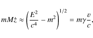
where we have used (8) and
![\begin{displaymath}\gamma =\left[ 1-\left( \frac{v}{c}\right) ^{2}\right] ^{-1/2}=\frac{E}{mc^{2}},
\end{displaymath}](/articles/aa/full_html/2010/07/aa13678-09/img193.png)
is the Lorentz factor. Hence, asymptotically, the speed of the particle is
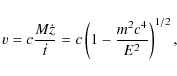
which is ultrarelativistic if
4 Incoming particles
We describe as ``incoming particles'' the particles, with parameters
![]() ,
,
![]() ,
and
,
and
![]() ,
coming into
the ergosphere following unbound geodesics and having a turning point in z(i.e. such that
,
coming into
the ergosphere following unbound geodesics and having a turning point in z(i.e. such that
![]() ). Such turning points {
). Such turning points {![]() ,
z4} are defined as solutions of the equation
,
z4} are defined as solutions of the equation
| (50) |
where
| N2 = Pz - S | (51) |
is the relevant factor in the numerator of the right side of Eq. (21). As remarked earlier we need only consider
![\begin{figure}
\par\includegraphics[width=8cm]{AA-2009-13678-fig3.eps}
\end{figure}](/articles/aa/full_html/2010/07/aa13678-09/img213.png)
|
Figure 3:
Penrose process. Plots of the ingoing particle (dashed line) coming
asymptotically, for
|
| Open with DEXTER | |
A test particle with parameters
![]() ,
,
![]() ,
and
,
and
![]() coming from infinity (in practice from the accretion
disk) parallel to z=0 towards the axis of the black hole corresponds to a
geodesic which, in the limit
coming from infinity (in practice from the accretion
disk) parallel to z=0 towards the axis of the black hole corresponds to a
geodesic which, in the limit
![]() ,
has an asymptote
defined by z=z1= constant where z1 is the impact parameter.
Therefore it is a limit-incoming particle with z<z1,
,
has an asymptote
defined by z=z1= constant where z1 is the impact parameter.
Therefore it is a limit-incoming particle with z<z1, ![]() ,
,
![]() ,
,
![]() .
In the limit
.
In the limit
![]() ,
,
![]() ,
so the tangent has to be parallel to the
,
so the tangent has to be parallel to the ![]() axis and Eq. (27) produces
axis and Eq. (27) produces
We have plotted in Fig. 3 (see Sect. 5) an example of a geodesic of an incoming particle. We see that, unlike
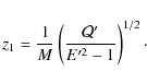
For a given
![]() ,
the most energetic incoming particles
are those with a small impact parameter z1, near to zero. Hence only a
thin slice of the accretion disk can participate with the greatest
efficiency in producing Penrose processes leading to the most intense
possible jet. The point where the ergosphere surface intersects the z axis
is
,
the most energetic incoming particles
are those with a small impact parameter z1, near to zero. Hence only a
thin slice of the accretion disk can participate with the greatest
efficiency in producing Penrose processes leading to the most intense
possible jet. The point where the ergosphere surface intersects the z axis
is
![]() .
The value of
.
The value of ![]() ,
for the incoming particles, does not
play a role like that of
,
for the incoming particles, does not
play a role like that of
![]() for the outgoing particles (compare Eq. (40) to Eq. (52)).
for the outgoing particles (compare Eq. (40) to Eq. (52)).
5 Penrose process and plotting of geodesics
To make a jet using the geodesics discussed above, we would have to assume
that incoming particles arrive in the ergosphere and undergo a Penrose
process. As mentioned earlier, in its original version (Penrose 1969), each
particle may be decomposed into two subparticles and one of them may cross
the horizon and fall irreversibly into the BH, while the other is ejected to
the exterior of the ergosphere; or the incoming particle may collide with
another particle resulting in one plunging into the BH and the other being
ejected to the exterior. The second case can correspond to a creation of
particles, say ![]() and
and ![]() from an incoming photon (
from an incoming photon (![]() )
interacting with another inside the ergosphere. We do not present here all
the possible cases, which are exhaustively studied, especially for AGN, in
Williams (1995,2004). There is also observational evidence for a close
correlation between the disappearance of the unstable inner accretion disk
and some subsequent ejections from microquasars such as GRS 1915+1105 (Mirabel & Rodriguez 1999,1994), which from our point of view could correspond to the
instability causing disk material to fall through the ergosphere and to then
give rise to a burst of ejecta from Penrose-like processes. Here we are
mainly interested in the outgoing particles which follow geodesics that tend
asymptotically towards a parallel to the z axis, as described in the
earlier Sect. 3. These events are closely dependent on the
possibilities allowed by the conservation equations. In the case when the
incoming particle splits into two (Rees et al. 1976), the conservation
equations of the energy and angular momentum are
)
interacting with another inside the ergosphere. We do not present here all
the possible cases, which are exhaustively studied, especially for AGN, in
Williams (1995,2004). There is also observational evidence for a close
correlation between the disappearance of the unstable inner accretion disk
and some subsequent ejections from microquasars such as GRS 1915+1105 (Mirabel & Rodriguez 1999,1994), which from our point of view could correspond to the
instability causing disk material to fall through the ergosphere and to then
give rise to a burst of ejecta from Penrose-like processes. Here we are
mainly interested in the outgoing particles which follow geodesics that tend
asymptotically towards a parallel to the z axis, as described in the
earlier Sect. 3. These events are closely dependent on the
possibilities allowed by the conservation equations. In the case when the
incoming particle splits into two (Rees et al. 1976), the conservation
equations of the energy and angular momentum are
We know from Eq. (29) that for the outgoing particles we study
We have plotted numerically the geodesics for incoming, outgoing and falling particles with the following values for the parameters: a/M=1/2,
![\begin{displaymath}z^{2}=\left\{ 1-\rho _{\rm e}^{2}\left[ 1-\left( \frac{\rho }...
...} \left[ 1-\left( \frac{\rho }{\rho _{\rm e}}\right) \right] ,
\end{displaymath}](/articles/aa/full_html/2010/07/aa13678-09/img239.png)
|
(56) |
and they produce for the asymptotes of the outgoing particles
The exhibition of these numerical solutions with an outgoing geodesic which
leaves the ergosphere after the Penrose process and has vertical asymptote
with the value ![]() precisely equal to Eq. (40) confirms that a model
based on such geodesics is possible.
precisely equal to Eq. (40) confirms that a model
based on such geodesics is possible.
6 Implications for jet formation
We have shown that to obtain a jet of particles close to the rotation axis,
it must be formed from particles with (almost) zero angular momentum, Lz=0. If we consider only particles with Lz=0, there is among them a subset
which give a perfectly collimated jet, i.e. a set of geodesics exactly
parallel to the axis: for each allowed value of
![]() they form a
ring of radius
they form a
ring of radius
![\begin{displaymath}\rho_{1}= \rho_{\rm e}\left[ 1+\frac{\mathcal{Q}}{a^{2}(E^{2}-1)}\right]^{1/2},
\end{displaymath}](/articles/aa/full_html/2010/07/aa13678-09/img242.png)
|
(57) |
whwre
We note that all other geodesics with Lz=0 will spread out from the axis
along lines ![]() .
An astrophysical jet will of course be of only finite
extent and not perfectly collimated, so it could include such geodesics for
suitably large K, as well as geodesics with a small
.
An astrophysical jet will of course be of only finite
extent and not perfectly collimated, so it could include such geodesics for
suitably large K, as well as geodesics with a small
![]() .
.
Thus forming a collimated jet of particles from a Penrose-like process, this jet having a narrow opening angle, for a rotating black hole without an electromagnetic field, depends on the initial distribution of particles leaving the ergosphere, or of some non-gravitational collimating force, even if we consider only particles with Lz=0.
On the other hand, outgoing particles with small energies, namely of the
order of their rest energy,
![]() ,
and
,
and
![]() have
asymptotes parallel to the z axis with
have
asymptotes parallel to the z axis with
![]() .
.
This predicted scale of the region of confined highly energetic particles
might provide a test if the accretion disk parameters provided values for
the BH mass and angular momentum, in a manner such as discussed in McClintock et al. (2006) and papers cited therein, and if the transverse linear scale
of the jet near the BH could be measured (Particles of equally high energy
may exist in
![]() but will spread out away from the axis).
but will spread out away from the axis).
Let us make a brief qualitative remark about the observability of the two
species, (a) and (b), of geodesics outgoing from the ergosphere, studied in
Sect. 3 (after Eq. (45)). As illustrated by the Fig. 2, for each fixed value
of ![]() there is one (b)-geodesic only, which is the limit of many
(one infinity of) (a)-geodesics when the turning point tends to the infinity
(
there is one (b)-geodesic only, which is the limit of many
(one infinity of) (a)-geodesics when the turning point tends to the infinity
(
![]() ,
,
![]() ). However, the
(a)-type geodesics, though much more numerous than the (b)-type geodesics,
are, directly or indirectly (i.e. by radiation, if charged), much more
difficult to observe.
). However, the
(a)-type geodesics, though much more numerous than the (b)-type geodesics,
are, directly or indirectly (i.e. by radiation, if charged), much more
difficult to observe.
Indeed, contrary to the set of (b)-particles framing the jet in one
direction (collimation along the poles), the (a)-particles ejected from the
ergosphere along unbound geodesics at lower latitudes are dispersed into the
whole 3D-space (![]() steradians). The (a)-particles never produce a beam
into one privileged direction but instead dilute in the whole space.
Observed from the infinity in one line of sight (
steradians). The (a)-particles never produce a beam
into one privileged direction but instead dilute in the whole space.
Observed from the infinity in one line of sight (
![]() ,
,
![]() ), one single (a)-particle could directly be detected. While, from
the infinity in the line of sight z (
), one single (a)-particle could directly be detected. While, from
the infinity in the line of sight z (![]() ,
,
![]() ), the
observer will see one infinity (each point of the perimeter of the circle of
radius
), the
observer will see one infinity (each point of the perimeter of the circle of
radius ![]() )
of (b)-particles. The result is reinforced when we
extend it to all the possible values of
)
of (b)-particles. The result is reinforced when we
extend it to all the possible values of ![]() .
Encircling the foot of
the (b)-jet, the (a)-particles frame a gerb, from the basis of which a
possible indirect effect of isotropic radiation emission (from accelerated
charged particles) could be observed, during the jet eruption.
.
Encircling the foot of
the (b)-jet, the (a)-particles frame a gerb, from the basis of which a
possible indirect effect of isotropic radiation emission (from accelerated
charged particles) could be observed, during the jet eruption.
Besides, by their dispersion, the pressure the (a)-particles locally exert on the ambient medium is much weaker than the pressure exerted by the numerous coherent (b)-particles of the jet (a narrow parallel beam is more incisive). The (a)-particles are probably more rapidly thermalised than the (b)-particles of the jet. So, one might expect that many particles ejected at lower latitudes never attain infinity (neither the height of the jet), and most of them feed the medium, framing a halo around the BH, falling inside again, or returning to the accretion disk.
We noted also that geodesics with
![]() can be asymptotic to lines
with constant
can be asymptotic to lines
with constant ![]() .
These asymptotes allow us to define another type of
jet which is bigger and less collimated than the previous one. It is
interesting to remark that recent observations (Sheth et al. 2003; Sauty et al. 2002)
suggest the existence of two different types of jets precisely of these
sorts, i.e. narrowly and broadly collimated.
.
These asymptotes allow us to define another type of
jet which is bigger and less collimated than the previous one. It is
interesting to remark that recent observations (Sheth et al. 2003; Sauty et al. 2002)
suggest the existence of two different types of jets precisely of these
sorts, i.e. narrowly and broadly collimated.
There exists an ensemble of geodesics that tend asymptotically to these
conical characteristics. The unbounded geodesics have mainly been discussed,
however, by using Boyer-Lindquist coordinates r and ![]() by the
majority of authors. If we rewrite our results, using these coordinates, we
may interpret our results and compare to those of other authors. However, as
we show below, these coordinates are not as well-suited to the issues we
have discussed.
by the
majority of authors. If we rewrite our results, using these coordinates, we
may interpret our results and compare to those of other authors. However, as
we show below, these coordinates are not as well-suited to the issues we
have discussed.
Geodesics with
![]() may reach low values of
may reach low values of ![]() ,
if b2is large enough, but must be bounded away from
,
if b2is large enough, but must be bounded away from
![]() (i.e.
(i.e. ![]() or
or
![]() ), since those values would imply
), since those values would imply
![]() ,
from Eq. (3), (cf. Chandrasekhar 1983, p. 348). In practice this means
that a narrow jet along the axis must be composed of particles with very
small Lz. Particles with non-zero Lz could only lie within a jet
with bounded
,
from Eq. (3), (cf. Chandrasekhar 1983, p. 348). In practice this means
that a narrow jet along the axis must be composed of particles with very
small Lz. Particles with non-zero Lz could only lie within a jet
with bounded ![]() for a limited distance, because large enough z would
imply
for a limited distance, because large enough z would
imply
![]() .
If
.
If
![]() ,
the orbits reverse the
sign of
,
the orbits reverse the
sign of
![]() and reach the equatorial plane, and would thus be
expected to be absorbed by the accretion disk. For
and reach the equatorial plane, and would thus be
expected to be absorbed by the accretion disk. For
![]() they
are confined to a band of values of
they
are confined to a band of values of ![]() given by the roots of S2=0.
These are the ``vortical'' trajectories of de Felice et al. (de Felice & Calvani 1972; de Felice & Carlotto 1997; de Felice & Curir 1992). Depending on the maximum opening angle
given by the roots of S2=0.
These are the ``vortical'' trajectories of de Felice et al. (de Felice & Calvani 1972; de Felice & Carlotto 1997; de Felice & Curir 1992). Depending on the maximum opening angle ![]() ,
these may still hit, and presumably be absorbed by, a thick accretion disk
(de Felice & Curir 1992). Such orbits can be adequately populated by Penrose-like
processes (Williams 1995,2004), and might undergo processes which reduce the
opening angle (de Felice & Carlotto 1997; de Felice & Curir 1992). A jet composed of such particles would
tend to be hollow and would have a larger radius
,
these may still hit, and presumably be absorbed by, a thick accretion disk
(de Felice & Curir 1992). Such orbits can be adequately populated by Penrose-like
processes (Williams 1995,2004), and might undergo processes which reduce the
opening angle (de Felice & Carlotto 1997; de Felice & Curir 1992). A jet composed of such particles would
tend to be hollow and would have a larger radius ![]() at large z than is
obtained for orbits with Lz=0, and hence be observationally
distinguishable. The presence of these escaping trajectories spiralling
round the polar axis can be associated with the gravitomagnetic effects due
to the rotation of the hole, one of whose consequences is that even curves
with Lz=0 have a non-zero
at large z than is
obtained for orbits with Lz=0, and hence be observationally
distinguishable. The presence of these escaping trajectories spiralling
round the polar axis can be associated with the gravitomagnetic effects due
to the rotation of the hole, one of whose consequences is that even curves
with Lz=0 have a non-zero
![]() at finite
distances.
at finite
distances.
Thus although an infinitely extended jet of bounded ![]() radius would
only contain particles with Lz=0, which we would expect to be a set of
measure zero among all particles ejected, we shall consider this as a good
model even for real jets. In practice, interactions with other forces and
objects, which would affect the jet both by gravitational and other forces,
have to be taken into account once the jet is well away from the BH, and
these influences might or might not improve the collimation. In (de Felice & Carlotto 1997), the authors discussed possible improved collimation for particles
of low Lz using forces which have a timescale long compared with the
dynamical timescale of the geodesics, and which act to move particles to new
geodesics with changed parameters. It should be noted that if the object
producing the jet is modelled as a rotating black hole, production of a
collimated jet only arises naturally if the object throws out energetic
particles with low Lz, since our discussion shows that other particles
cannot join such a jet unless there is some other strong collimating
influence away from the BH.
radius would
only contain particles with Lz=0, which we would expect to be a set of
measure zero among all particles ejected, we shall consider this as a good
model even for real jets. In practice, interactions with other forces and
objects, which would affect the jet both by gravitational and other forces,
have to be taken into account once the jet is well away from the BH, and
these influences might or might not improve the collimation. In (de Felice & Carlotto 1997), the authors discussed possible improved collimation for particles
of low Lz using forces which have a timescale long compared with the
dynamical timescale of the geodesics, and which act to move particles to new
geodesics with changed parameters. It should be noted that if the object
producing the jet is modelled as a rotating black hole, production of a
collimated jet only arises naturally if the object throws out energetic
particles with low Lz, since our discussion shows that other particles
cannot join such a jet unless there is some other strong collimating
influence away from the BH.
However previous authors have not pointed out the existence of asymptotes
![]() ,
presumably because they are less obvious when using
coordinates r and
,
presumably because they are less obvious when using
coordinates r and ![]() .
In fact, considering
.
In fact, considering
![]() ,
the
expressions (12) and (15) produce
,
the
expressions (12) and (15) produce
![]() ,
,
![]() and
and
![]() .
With these expansions it is clear
that in the limit
.
With these expansions it is clear
that in the limit ![]() one would have to take the limit of
one would have to take the limit of
![]() to allow
to allow ![]() to be determined.
to be determined.
In the same vein, to find the values of asymptotes
![]() near the
equatorial plane
near the
equatorial plane
![]() for the incoming particles (see Eq. (52))
one has to study
for the incoming particles (see Eq. (52))
one has to study
![]() if one uses the coordinates r and
if one uses the coordinates r and ![]() .
In fact, one finds for the asymptotic expansion
.
In fact, one finds for the asymptotic expansion
![]() the
following expressions,
the
following expressions,
![]() ,
,
![]() and
and
![]() .
.
7 Conclusion
Our main results are the following.
There are projections of geodesics all over the meridional planes. Among
these geodesics there are some, with vertical asymptotes parallel to zwhich can form a perfectly collimated jet. There are, as well, geodesics
with horizontal asymptotes parallel to the radial coordinate ![]() ,
that
can represent the paths of incoming particles leaving the accretion disk.
,
that
can represent the paths of incoming particles leaving the accretion disk.
These two types of geodesics have intersection points that can be situated
inside the ergosphere. At these points a Penrose process can take place,
producing the ejection of particles along the axis with bigger energies than
the energies of incoming particles close to the equatorial plane. The
energies of outgoing particles are significantly larger than the ones of the
incident particles for the asymptotically vertical geodesics near the scale a/M of the ergosphere diameter in the coordinate ![]() ,
so such particles
can show collimation around the surface of a tube of diameter 2a/M centred
on the axis of symmetry. Such collimated outgoing particles have to have a
zero orbital momentum Lz=0, which implies, from the Penrose process,
that the incoming particles have a negative orbital momentum,
,
so such particles
can show collimation around the surface of a tube of diameter 2a/M centred
on the axis of symmetry. Such collimated outgoing particles have to have a
zero orbital momentum Lz=0, which implies, from the Penrose process,
that the incoming particles have a negative orbital momentum,
![]() .
Thus the jet has to be fed from incoming particles with retrograde
orbits in the accretion disk. There is evidence for the existence of
substantial counterrotating parts of accretion disks (Koide et al. 2000; Thakar et al. 1997), and such counterrotations could explain the
viscosity inducing the instabilities which trigger the falling of matter
towards the ergosphere. It is now known (Mirabel & Rodriguez 1994,1999; Mirabel 2006) that
there is a close connection between instabilities in the accretion disk and
the genesis of jets for quasars and microquasars.
.
Thus the jet has to be fed from incoming particles with retrograde
orbits in the accretion disk. There is evidence for the existence of
substantial counterrotating parts of accretion disks (Koide et al. 2000; Thakar et al. 1997), and such counterrotations could explain the
viscosity inducing the instabilities which trigger the falling of matter
towards the ergosphere. It is now known (Mirabel & Rodriguez 1994,1999; Mirabel 2006) that
there is a close connection between instabilities in the accretion disk and
the genesis of jets for quasars and microquasars.
The most energetic incoming particles are those near the equatorial plane.
Hence the incoming particles which produce the most energetic outgoing
particles by a Penrose process in the ergosphere, whose maximum size is
![]() ,
are those with angular momentum
,
are those with angular momentum
![]() and a very small
impact parameter z1.
and a very small
impact parameter z1.
Also, the limiting diameter of the core of a perfectly collimated jet
depends upon the size of the ergosphere. The effective thickness of this
part of the jet in this case is of the order of
![]() .
.
Our idealised model is based on the well-behaved vacuum stationary exact
solution of Einstein's equations with axial symmetry, namely the Kerr
metrics, which does not take into account the ambient medium. Though this
medium is very dilute, it plays a non-negligible role on the more complex
global scenario for jets like progressive widening of the beam, advent of
knots, lobes, etc. However, for the scenario that we are here concerned,
namely the beginning of the jet (parsec scale for microquasars,while some
hundred parsecs for AGN, depending on the BH mass), where it is strongly
collimated, our approximation of test-particles along geodesics is relevant.
Indeed, the observed jets stemming from active galactic nuclei ejected along
the polar axis have ultrarelativistic speeds, typically
vj=0.99995c.
The ejected particles, forming the jets, are thermalized with temperatures
of the order 105 K (Filloux 2009) producing a lateral force from the
pressure gradient between the thermal energy of the particles in the outflow
and the low density enveloping medium (Punsly 1999a,b). The
internal particle trajectories to these jets expand laterally at the speed
of sound, being of the order
![]() km s-1 (Filloux 2009), asymptotically
forming a conical shape with an opening angle of the order of the inverse
Mach number
km s-1 (Filloux 2009), asymptotically
forming a conical shape with an opening angle of the order of the inverse
Mach number
![]() radians. As we can see (Punsly 1999b,
Appendix), the more realistic trajectories corresponding to such corrective
terms represent only a small perturbation to the geodesics.
radians. As we can see (Punsly 1999b,
Appendix), the more realistic trajectories corresponding to such corrective
terms represent only a small perturbation to the geodesics.
The model that we present to explain the formation and collimation of jets arises essentially from relativistic strong gravitational field phenomena without resort to electromagnetic phenomena. From this point of view the model could be interesting also for understanding observational evidence of neutral particles emitted from the inner jet itself. For example, the recent observations of Ultra High Energy Cosmic Rays (difficult to explain, implying neutral particles such as neutrinos, or H or Fe atoms, etc. Auger 2007a,b; Dermer et al. 2009; and HESS collab. 2009, and references therein) is a new challenge. To explain the Very High Energy of such neutral (massive) particles, especially neutrinos (Auger 2007a,b, which are able to travel freely over large distances), our model very naturally suggests that they could be directly coming from the collimated inner jet, which would privilege sources (BH) with rotational z-axis along the line of sight of the observation. Massless particles (photons) would be emitted by charged particles accelerated along the collimated inner jet (Dermer et al. 2009; HESS collab. 2009), which would privilege sources (BH) with rotational z-axis perpendicular to the line of sight of the observation.
Our model is sufficiently general to fit various types of observed jets,
like GRB, jets ejected from AGN or from microquasars, whenever they are
energetic enough to be explained by just a rotating black hole fed by an
accretion disk in an axisymmetric configuration. The main drawback is the
need to preferentially populate the geodesics which can form such collimated
jets. Work is in progress on this question to determine a possible
confrontation of the model with observations. Our preliminary studies led
us to understand the fundamental role of the function P(r) of the
geodesics equations (See Eqs. (2) and (19)). As an example, in the special case
where the equation P(r)=0 has a real double root, there exist only two
narrow ranges of ![]() values for large values of E. In this case,
we can evaluate from the power, for example of radio loud extragalactic jets
(Willott et al. 1999), or of microquasars jets (Fender et al. 2004), the particle
density, the mean kinetic energy by particle, the mean velocity and the
Lorentz factor of the jets. These results, since they require a long
presentation, deserve a separate paper which is under preparation.
values for large values of E. In this case,
we can evaluate from the power, for example of radio loud extragalactic jets
(Willott et al. 1999), or of microquasars jets (Fender et al. 2004), the particle
density, the mean kinetic energy by particle, the mean velocity and the
Lorentz factor of the jets. These results, since they require a long
presentation, deserve a separate paper which is under preparation.
The existence of vacuum solutions of the Einstein equations of Kerr type but with a richer, not connected, topological configuration of the ergosphere (see Gariel et al. 2002, Figs. 7-10), allows us to propose the existence of double jets, because they are expected to come out from the ergosphere. These bipolar jets have been observed (see for instance Skinner et al. 1997; Sahai et al. 1998, Fig. 1; Fargion 2003, Fig. 2; and Kwok et al. 1998) and could be naturally interpreted in a generalization of our model.
AcknowledgementsWe are grateful to Dr. Reva Kay Williams for correspondence concerning her papers and for further references, and to Prof. J. Bicák for bringing (Bicák et al. 1993) to our attention.
References
- Auger collaboration 2007, Science, 318, 939 [Google Scholar]
- Auger collaboration 2007, Astropart. Phys., 29, 188, erratum: ibid 2008, 30, 45 [NASA ADS] [CrossRef] [Google Scholar]
- Bicák, J., Semerák, O., & Hadrava, P. 1993, MNRAS, 263, 545 [NASA ADS] [Google Scholar]
- Blandford, R. D., & Znajek, R. L. 1977, MNRAS, 179, 433 [NASA ADS] [CrossRef] [Google Scholar]
- Carter, B. 1968, Phys. Rev., 174, 1559 [NASA ADS] [CrossRef] [Google Scholar]
- Chandrasekhar, S. 1983, The Mathematical Theory of Black Holes (Oxford: Oxford University Press), 346 [Google Scholar]
- de Felice, F., & Calvani, M. 1972, Nuovo Cimento B, 10, 447 [NASA ADS] [Google Scholar]
- de Felice, F., & Carlotto, L. 1997, ApJ, 481, 116 [NASA ADS] [CrossRef] [Google Scholar]
- de Felice, F., & Curir, A. 1992, Class. Quantum Grav., 9, 1303 [NASA ADS] [CrossRef] [Google Scholar]
- de Felice, F., & Zanotti, O. 2000, Gen. Rel. Grav., 32, 1449 [NASA ADS] [CrossRef] [Google Scholar]
- Dermer, C. D., Razzaque, S., Finke, J. D., & Atoyan, A. 2009, New J. Phys., 11, 065016 [Google Scholar]
- Fargion, D. 2003, Puzzling afterglow's oscillations in GRBs and SGRs: tails of precessing jets, Tech. Rep., contribution to the Vulcano conference [arXiv:astro-ph/0307314] [Google Scholar]
- Fender, R. P., Belloni, T. M., & Gallo, E. 2004, MNRAS, 355, 1105 [NASA ADS] [CrossRef] [Google Scholar]
- Filloux, C. 2009, Ph.D. Thesis, Université de Nice Sophia-Antipolis, France [Google Scholar]
- Gariel, J., Marcilhacy, G., & Santos, N. O. 2002, Class. Quantum Grav., 19, 2157 [NASA ADS] [CrossRef] [Google Scholar]
- Herrera, L., & Santos, N. O. 2007, Astrophys. Space Sci., 310, 251 [NASA ADS] [CrossRef] [Google Scholar]
- HESS collaboration 2009, ApJ, 695, L40 [NASA ADS] [CrossRef] [Google Scholar]
- Hughson, L. P., Penrose, R., Sommers, P., & Walker, M. 1972, Commun. math. phys., 27, 303 [NASA ADS] [CrossRef] [Google Scholar]
- Koide, S., Meier, D. L., Shibata, K., & Kudoh, T. 2000, ApJ, 536, 668 [NASA ADS] [CrossRef] [Google Scholar]
- Kwok, S., Su, K. Y. L., & Hrivnak, B. J. 1998, ApJ, 501, L117 [NASA ADS] [CrossRef] [Google Scholar]
- Livio, M. 1999, Phys. Rep., 311, 225 [NASA ADS] [CrossRef] [Google Scholar]
- McClintock, J. E., Shafee, R., Narayan, R., et al. 2006, ApJ, 652, 518 [NASA ADS] [CrossRef] [Google Scholar]
- Mirabel, I. F. 2006, in Black holes: from stars to galaxies, Across the Range of Masses, concluding Remarks, Proc. IAU Symp., 238 [Google Scholar]
- Mirabel, I. F., & Rodriguez, L. F. 1994, Nature, 371, 46 [NASA ADS] [CrossRef] [Google Scholar]
- Mirabel, I. F., & Rodriguez, L. F. 1999, ARA&A, 37, 409 [NASA ADS] [CrossRef] [Google Scholar]
- O'Neill, B. 1995, The Geometry of Kerr Black Holes (Wellesley, Massachusetts: A K Peters Ltd.) [Google Scholar]
- Opher, R., Santos, N. O., & Wang, A. 1996, J. Math. Phys., 37, 1982 [NASA ADS] [CrossRef] [Google Scholar]
- Penrose, R. 1969, Rivista del Nuovo Cimento, Numero Special 1, 252 [Google Scholar]
- Piran, T., Kumar, P., Panaitescu, A., & Piro, L. 2001, ApJ, 560, L167 [NASA ADS] [CrossRef] [Google Scholar]
- Piran, T., & Shaham, J. 1977, Phys. Rev. D, 16, 1615 [NASA ADS] [CrossRef] [Google Scholar]
- Punsly, B. 1999a, ApJ, 527, 609 [NASA ADS] [CrossRef] [Google Scholar]
- Punsly, B. 1999b, ApJ, 527, 624 [NASA ADS] [CrossRef] [Google Scholar]
- Punsly, B. 2001, Black Hole Gravitohydromagnetics (Berlin and Heidelberg: Springer-Verlag) [Google Scholar]
- Punsly, B., & Coroniti, F. V. 1990a, ApJ, 354, 583 [NASA ADS] [CrossRef] [Google Scholar]
- Punsly, B., & Coroniti, F. V. 1990b, ApJ, 350, 518 [NASA ADS] [CrossRef] [Google Scholar]
- Rees, M., Ruffini, R., & Wheeler, J. A. 1976, Black Holes, Gravitational Waves and Cosmology: An Introduction to Current Research (New york: Gordon and Breach Science Publishers) [Google Scholar]
- Sahai, R., Trauger, J. T., Watson, A. M., et al. 1998, ApJ, 493, 301 [NASA ADS] [CrossRef] [Google Scholar]
- Sauty, C., Tsinganos, K., & Trussoni, E. 2002, in Relativistic Flows in Astrophysics, Springer Lecture Notes in Physics, ed. A. W. Guthmann, M. Georganopoulos, A. Marcowith, & K. Manolakou (Berlin and Heidelbergn: Springer-Verlag), 589, 41 [arXiv:astro-ph/0108509] [Google Scholar]
- Sharp, N. A. 1979, Gen. Rel. Grav., 10, 659 [NASA ADS] [CrossRef] [Google Scholar]
- Sheth, K., Frail, D. A., White, S., et al. 2003, ApJ, 595, L33 [NASA ADS] [CrossRef] [Google Scholar]
- Skinner, C. J., Meixner, M., Barlow, M. J., et al. 1997, A&A, 328, 290 [NASA ADS] [Google Scholar]
- Stewart, J. M., & Walker, M. 1974, Springer Tracts in Modern Physics, Black holes: the outside story (Berlin: Springer), 69 [Google Scholar]
- Thakar, A. R., Ryden, B. S., Jore, K. P., & Broeils, A. H. 1997, ApJ, 479, 702 [NASA ADS] [CrossRef] [Google Scholar]
- Willott, C., Rawlings, S., Blundell, K., & Lacy, M. 1999, MNRAS, 309, 1017 [NASA ADS] [CrossRef] [Google Scholar]
- Wilkins, D. C. 1972, Phys. Rev. D, 5, 814 [NASA ADS] [CrossRef] [Google Scholar]
- Williams, R. K. 1995, Phys. Rev. D, 51, 5387 [NASA ADS] [CrossRef] [Google Scholar]
- Williams, R. K. 2004, ApJ, 611, 952 [NASA ADS] [CrossRef] [Google Scholar]
Footnotes
- ... particle
![[*]](/icons/foot_motif.png)
- An alternative interpretation is to assume that for a
particle of mass m,
the affine parameter
 has been used (Williams
1995; Wilkins
1972).
has been used (Williams
1995; Wilkins
1972).
All Figures
|
|
Figure 1:
Plot of the surface
|
| Open with DEXTER | |
| In the text | |
|
|
Figure 2:
Plots of geodesics obeying Eq. (21), showing
the turning points. From left to right these curves start at
|
| Open with DEXTER | |
| In the text | |
|
|
Figure 3:
Penrose process. Plots of the ingoing particle (dashed line) coming
asymptotically, for
|
| Open with DEXTER | |
| In the text | |
Copyright ESO 2010
Current usage metrics show cumulative count of Article Views (full-text article views including HTML views, PDF and ePub downloads, according to the available data) and Abstracts Views on Vision4Press platform.
Data correspond to usage on the plateform after 2015. The current usage metrics is available 48-96 hours after online publication and is updated daily on week days.
Initial download of the metrics may take a while.