| Issue |
A&A
Volume 515, June 2010
|
|
|---|---|---|
| Article Number | A46 | |
| Number of page(s) | 8 | |
| Section | The Sun | |
| DOI | https://doi.org/10.1051/0004-6361/200913487 | |
| Published online | 08 June 2010 | |
The effect of longitudinal flow on resonantly damped kink oscillations
J. Terradas1 - M. Goossens1 - I. Ballai2
1 - Centre Plasma Astrophysics and Leuven Mathematical Modeling and
Computational Science Center, Katholieke Universiteit Leuven, Celestijnenlaan
200B, 3001 Leuven, Belgium
2 -
Solar Physics and Space Plasmas Research Centre (SP2RC),
Department of Applied Mathematics, University of Sheffield, Hounsfield
Road, Hicks Building, Sheffield, S3 7RH, England, UK
Received 16 October 2009 / Accepted 1 March 2010
Abstract
Context. The most promising mechanism acting towards damping
the kink oscillations of coronal loops is resonant absorption. In this
context most of previous studies neglected the effect of the obvious
equilibrium flow along magnetic field lines. The flows are in general
sub-Alfvénic and hence comparatively slow.
Aims. Here we investigate the effect of an equilibrium flow on
the resonant absorption of linear kink MHD waves in a cylindrical
magnetic flux tube with the aim of determining the changes in the
frequency of the forward and backward propagating waves and in the
modification of the damping times due to the flow.
Methods. A loop model with both the density and the longitudinal
flow changing in the radial direction is considered. We use the thin
tube thin boundary (TTTB) approximation in order to calculate the
damping rates. The full resistive eigenvalue problem is also solved
without assuming the TTTB approximation.
Results. Using the low ratio of flow and Alfvén speeds we derive
simple analytical expressions to the damping rate. The analytical
expressions are in good agreement with the resistive eigenmode
calculations.
Conclusions. Under typical coronal conditions the effect of the
flow on the damped kink oscillations is weak when the characteristic
scale of the density layer is similar or lower than the characteristic
width of the velocity layer. However, in the opposite situation the
damping rates can be significantly altered, specially for the backward
propagating wave which is undamped while the forward wave is
overdamped.
Key words: magnetohydrodynamics (MHD) - waves - magnetic fields - Sun: corona
1 Introduction
In space and solar plasmas flows are observed in high resolution on almost all temporal and spatial scales. Flows are ubiquitous in active region loops and the measurements of their velocities have been provided by instruments like SoHO (see Winebarger et al. 2002; Brekke et al. 1997), TRACE (see Winebarger et al. 2001) and more recently Hinode (see for example Ofman & Wang 2008; Chae et al. 2008; Terradas et al. 2008b). In general the flow speeds are low, and in most of the observations they are sub-Alfvénic, typically less that 10% of the Alfvén speed. The bulk motions are observed along magnetic field lines which outline coronal loops. These flows could be generated by some catastrophic cooling of coronal loops or are related to some siphon mechanism arising due to the difference in pressure at the loop footpoints. Since longitudinal steady flows carrying momentum and providing additional inertia are present in coronal loops it is necessary to study their effects on the transverse oscillations observed in these structures (see for example Nakariakov et al. 1999; Aschwanden et al. 1999). An effect which is of obvious importance for magnetohydrodynamic (MHD) wave theory of loops' dynamics is how the period and the damping time are modified by the flow.
Here we are interested in the damping of the fundamental kink mode due to resonant absorption, based on the transfer of energy from a global MHD wave to local resonant Alfvén waves, and in the way the efficiency of the mechanism is altered by a stationary flow. In the past, the influence of a velocity shear on this process due to a longitudinal flow has been studied by Hollweg et al. (1990); Peredo & Tataronis (1990), Erdélyi & Goossens (1996); Ruderman & Goossens (1995); Tirry et al. (1998); Erdélyi et al. (1995). More recently, Andries et al. (2000); Erdélyi & Taroyan (2003b); Andries & Goossens (2001); Erdélyi & Taroyan (2003a), have investigated in detail resonant flow instabilities which can occur for velocity shears significantly below the Kelvin-Helmholtz (KH) threshold. These instabilities are produced when the frequency of the forward propagating wave (propagating in the direction of the flow) shifts into the Doppler shifted continuum of the backward propagating wave. Under these conditions the mode becomes unstable and the flow acts at the resonant layer as an energy source. In most of the aforementioned studies it has been assumed that the wavelength is shorter or similar to the tube radius. This is not the case for standing kink oscillations in coronal loops which are precisely in the opposite regime, i.e., where the thin tube (TT) approximation is applicable.
In the present paper we extend the previous studies about resonant absorption in the presence of flow to the situation where the TT approximation is valid. We start by reviewing the properties of kink MHD waves in a homogeneous tube with an axial flow and study the nature of the waves, that change from being trapped to leaky and eventually become KH-unstable. Then we consider a non-uniform tube whose oscillation is damped by resonant absorption and investigate how the damping time is modified by the flow. In the following analysis three different approaches are implemented. Firstly, we use existing theoretical work, mainly by Goossens et al. (1992), to calculate the changes in the period and damping rates induced by the longitudinal flow using the thin tube thin boundary approximation (TTTB). Secondly, under the TTTB assumption we derive a linear analytical approximation to the damping rate and thirdly, solve the full resistive eigenvalue problem without the TTTB assumption. Reassuringly, we find that the three methods lead to essentially the same results.
2 Basic features: uniform tube
We consider what we can call the standard loop model, a cylindrical
axi-symmetric flux tube of radius R with a constant axial magnetic field B0and with a density contrast of
![]() where the indices ``i'' and ``e''
describe quantities inside and outside the loop, respectively. Inside the loop
there is an axial flow denoted by
where the indices ``i'' and ``e''
describe quantities inside and outside the loop, respectively. Inside the loop
there is an axial flow denoted by ![]() .
For simplicity we assume that there is
no flow outside the tube so that
.
For simplicity we assume that there is
no flow outside the tube so that
![]() .
We start by recalling the analytical
results obtained for a uniform loop (no transition layer) in the
.
We start by recalling the analytical
results obtained for a uniform loop (no transition layer) in the ![]() case.
It is well-known that the effect of the flow introduces a shift in the frequency
of waves and that the known expressions for the dispersion relation without flow
can be used by simply replacing the frequency
case.
It is well-known that the effect of the flow introduces a shift in the frequency
of waves and that the known expressions for the dispersion relation without flow
can be used by simply replacing the frequency ![]() by its Doppler-shifted
counterpart,
by its Doppler-shifted
counterpart,
![]() ,
k being the wavenumber along the tube. The
dispersion relation of MHD waves was derived in Goossens et al. (1992)
(see also Terra-Homem et al. 2003; Soler et al. 2008). In the TT approximation (
,
k being the wavenumber along the tube. The
dispersion relation of MHD waves was derived in Goossens et al. (1992)
(see also Terra-Homem et al. 2003; Soler et al. 2008). In the TT approximation (![]() )
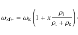
Goossens et al. (1992) found that the frequency of the kink MHD wave
modified by the flow,
)
Goossens et al. (1992) found that the frequency of the kink MHD wave
modified by the flow,
![]() ,
(see their equation Eq. [83]) is given by
,
(see their equation Eq. [83]) is given by
where
In the above equation
with
The frequency
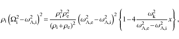
The second term of Eq. (1) contains the condition for the
Kelvin-Helmholtz instability which occurs for any velocity shear in absence of a
magnetic field. When magnetic fields are present it is straightforward to see
that the square root in Eq. (1) is negative when the flow is faster
than the critical value given by
The above condition means that fast flows compared to the internal Alfvén speed are required for the Kelvin-Helmholtz instability to occur (see also Chandrasekhar 1961; Ferrari et al. 1981). An equivalent problem has been studied in the context of propagating transverse waves in coronal jets by Vasheghani Farahani et al. (2009). These authors have also found that in the observationally determined range of parameters, the waves do not undergo either to the KHI or the negative energy wave instability.
![\begin{figure}
\par\subfigure[]{\includegraphics[width=8cm,clip]{13487f1a.eps} }
\subfigure[]{\includegraphics[width=8cm,clip]{13487f1b.eps} }
\end{figure}](/articles/aa/full_html/2010/07/aa13487-09/img29.png)
|
Figure 1:
a) Real and b) imaginary part of the frequency of
the forward (
|
| Open with DEXTER | |
However, before the Kelvin-Helmholtz instability occurs, it may happen that the
frequency of the modes is above the external cut-off frequency (
![]() ), meaning that the wave becomes leaky. The forward propagating wave
becomes leaky when the following condition is satisfied
), meaning that the wave becomes leaky. The forward propagating wave
becomes leaky when the following condition is satisfied
Similar to the KH-instability, fast flows are required to generate a leaky wave. Contrary to the static situation studied by Goossens et al. (2009), in the presence of flow an underdense loop is not required to have leaky modes when
The decrement is proportional to the square of k R (
An example of the dependence of the real (
![]() )
and imaginary (
)
and imaginary (![]() )
part of the frequency of the modes (fundamental forward and backward waves) on
the flow is shown in Fig. 1 for a particular equilibrium
configuration (L=100R,
)
part of the frequency of the modes (fundamental forward and backward waves) on
the flow is shown in Fig. 1 for a particular equilibrium
configuration (L=100R,
![]() ). The domains where waves become
leaky or when a KHI occurs are clearly shown. When the frequencies of the two
modes merge for increasing velocity shear (
). The domains where waves become
leaky or when a KHI occurs are clearly shown. When the frequencies of the two
modes merge for increasing velocity shear (![]() )
the system becomes unstable.
However, note that the forward wave is always leaky before the system
becomes KH unstable (compare also Eq. (6) with Eq. (5)). It is
important to mention here that we have not considered here the Principal Leaky
Mode which is a very peculiar solution of the dispersion relation
(see Cally 1986,2003) and instead have focused on the modes than are trapped
for a the static background.
)
the system becomes unstable.
However, note that the forward wave is always leaky before the system
becomes KH unstable (compare also Eq. (6) with Eq. (5)). It is
important to mention here that we have not considered here the Principal Leaky
Mode which is a very peculiar solution of the dispersion relation
(see Cally 1986,2003) and instead have focused on the modes than are trapped
for a the static background.
Once we know the main effects of the flow on the kink MHD waves we need to know
in which regime of Fig. 1 we can match, for example, the
observed standing kink oscillations. The observations of flows in coronal loops
indicate that they are slow, therefore hereafter we focus on sub-Alfvénic
flows rather than the super-Alfvénic flows that might cause leakage and KH
instabilities. We concentrate on the regime
![]() ,
thus according to
the previous analysis both the forward and backward waves are always trapped.
This also prevents the presence of resonant flow instabilities which occur
when the frequency of the forward propagating wave shifts into the Doppler
shifted continuum of the backward propagating wave.
,
thus according to
the previous analysis both the forward and backward waves are always trapped.
This also prevents the presence of resonant flow instabilities which occur
when the frequency of the forward propagating wave shifts into the Doppler
shifted continuum of the backward propagating wave.
3 Waves in a Non-uniform tube
Now let us consider a tube with a smooth variation of density and flow across
the loop cross-section. In particular we consider the case when ![]() varies
from its internal value
varies
from its internal value
![]() to its external value
to its external value
![]() in the interval
[R-l/2,R+l/2] and the velocity changes from
in the interval
[R-l/2,R+l/2] and the velocity changes from ![]() to 0 in the interval
to 0 in the interval
![]() .
Under such conditions the process of resonant
absorption takes place and kink oscillations in coronal loops will damp
efficiently. The reader is referred to Goossens (2008) and references therein
for a detail review on this kink wave damping mechanism.
.
Under such conditions the process of resonant
absorption takes place and kink oscillations in coronal loops will damp
efficiently. The reader is referred to Goossens (2008) and references therein
for a detail review on this kink wave damping mechanism.
As in the previous Section we concentrate on propagating waves, the possible excitation of standing waves in the presence of flow is discussed later.
3.1 The TTTB approximation
In a non-uniform tube the imaginary part of the frequency (of the trapped
propagating modes) is different from zero due to mode conversion at the inhomogeneous
layer (
![]() ). Some time ago Goossens et al. (1992)
derived an expression for the damping rate in the thin tube and thin boundary
(
). Some time ago Goossens et al. (1992)
derived an expression for the damping rate in the thin tube and thin boundary
(![]() )
approximation for incompressible MHD waves. For compressible waves
in a magnetic cylinder, using the loop model considered here, we obtain exactly
the same expression, given by (see their Eq. (76))
)
approximation for incompressible MHD waves. For compressible waves
in a magnetic cylinder, using the loop model considered here, we obtain exactly
the same expression, given by (see their Eq. (76))
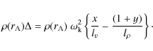
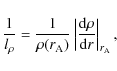
As usual
i.e. where there is a match between the Doppler shifted frequency and the local Alfvén frequency. It is assumed that the real part of the frequency of the resonantly damped mode is given by Eq. (1). From a physical point of view, the condition given by Eq. (9) means that the eigenmodes resonantly interact with the Alfvén continuum, which is Doppler shifted as a result of flow.
The factor ![]() in the denominator of Eq. (8) is
in the denominator of Eq. (8) is
which contains a term with the derivative of the flow in the radial direction, absent in the static situation, that can increase or decrease the value of
Given a particular density and velocity profile, the different variables in
Eq. (8) can be evaluated. For simplicity, we use the
well known sinusoidal profile for the density given by
This convenient profile has been used in many studies about resonant absorption (e.g. Terradas et al. 2006; Van Doorsselaere et al. 2004; Ruderman & Roberts 2002; Arregui et al. 2005). In order to make the mathematical approach more tractable we also assume that the variation of the flow speed is sinusoidal inside the loop layer, i.e.,
The flow is variable over a layer of thickness
![\begin{figure}
\par\includegraphics[width=8cm,clip]{13487f2.eps}
\end{figure}](/articles/aa/full_html/2010/07/aa13487-09/img51.png)
|
Figure 2:
Forward ( |
| Open with DEXTER | |
For the profiles given by Eqs. (11) and (12) it turns out that
Eq. (9) is a transcendental equation for the resonant position ![]() .
This equation is solved using standard numerical techniques. Depending on the
spatial scales of the density and velocity we distinguish two different regimes,
.
This equation is solved using standard numerical techniques. Depending on the
spatial scales of the density and velocity we distinguish two different regimes,
![]() and the asymptotic case
and the asymptotic case
![]() .
.
The analysis of the first situation is rather simple (see
also Peredo & Tataronis 1990), since the the forward propagating wave has always a single
resonant position in the range
![]() ,
while the resonant position of the
backward wave is situated in the range
,
while the resonant position of the
backward wave is situated in the range
![]() .
This behaviour is easily
understood from Fig. 2, where we have plotted the Doppler shifted
frequencies and the Alfvén frequency as a function of the radial coordinate.
The resonant positions are located at the intersection of
.
This behaviour is easily
understood from Fig. 2, where we have plotted the Doppler shifted
frequencies and the Alfvén frequency as a function of the radial coordinate.
The resonant positions are located at the intersection of ![]() with
with
![]() (see arrows). Note that Fig. 2 also shows that if the
Alfvén frequency is discontinuous (jump in density, l=0) there are no
resonances (implying no damping) since
(see arrows). Note that Fig. 2 also shows that if the
Alfvén frequency is discontinuous (jump in density, l=0) there are no
resonances (implying no damping) since ![]() will never intersect the curve
corresponding to
will never intersect the curve
corresponding to
![]() .
.
Once the resonant position ![]() is determined
is determined
![]() is evaluated
and we finally obtain the value of the damping rate
is evaluated
and we finally obtain the value of the damping rate ![]() (using
Eq. (8)). A useful quantity that we can calculate is the the damping per period, given by
(using
Eq. (8)). A useful quantity that we can calculate is the the damping per period, given by

|
(13) |
In this expression we use the real part of the frequency given by Eq. (1). In Fig. 3 (see solid lines)
![\begin{figure}
\par\includegraphics[width=8cm,clip]{13487f3.eps}
\end{figure}](/articles/aa/full_html/2010/07/aa13487-09/img63.png)
|
Figure 3:
Damping
per period as a function of the flow inside the loop for the forward (+) and
backward (-) propagating waves. The solid lines represent the analytical
results calculated using Eqs. (1) and (8). The dashed
lines are the approximations of the damping per period using
Eqs. (17) and (28). The dots represent the full
numerical solution of the resistive eigenvalue problem. The horizontal dotted
lines are the damping per period in the static situation. For the curves with
l/R=0.05, 0.1 we have used
|
| Open with DEXTER | |
In Fig. 4 we have represented the damping per period as a function of
![]() in units of loop radius for two different values of l/R. In this
plot, l, the characteristic scale of the density transition, is fixed (recall
we are still in the regime with
in units of loop radius for two different values of l/R. In this
plot, l, the characteristic scale of the density transition, is fixed (recall
we are still in the regime with
![]() ). For large values of
). For large values of
![]() compared to l we see that the dependence is quite weak with the
thickness of the flow profile. The forward propagating wave has a larger damping
per period than the backward propagating wave. However, when
compared to l we see that the dependence is quite weak with the
thickness of the flow profile. The forward propagating wave has a larger damping
per period than the backward propagating wave. However, when
![]() the situation is reversed. The curves cross and the forward propagating wave
is attenuated faster than the backward propagating wave, indicating that we are
at the threshold of a different regime.
the situation is reversed. The curves cross and the forward propagating wave
is attenuated faster than the backward propagating wave, indicating that we are
at the threshold of a different regime.
![\begin{figure}
\par\includegraphics[width=8cm,clip]{13487f4.eps}
\end{figure}](/articles/aa/full_html/2010/07/aa13487-09/img65.png)
|
Figure 4:
Damping per period for the forward and
backward propagating waves as a function of the width of the flow profile,
|
| Open with DEXTER | |
![\begin{figure}
\par\includegraphics[width=8cm,clip]{13487f5.eps}
\end{figure}](/articles/aa/full_html/2010/07/aa13487-09/img66.png)
|
Figure 5:
Forward ( |
| Open with DEXTER | |
Now let us concentrate on the situation when
![]() ,
i.e., we
investigate the case with a very steep profile for the equilibrium flow
velocity. This is different to the regime discussed earlier (
,
i.e., we
investigate the case with a very steep profile for the equilibrium flow
velocity. This is different to the regime discussed earlier (
![]() )
in several aspects. In Fig. 5 we have plotted a typical
example. It is easy to see that the forward wave can have now three different
resonant positions (see arrows). Apart from the resonance inside the
inhomogeneous velocity layer, the forward wave has two additional resonances,
one at
)
in several aspects. In Fig. 5 we have plotted a typical
example. It is easy to see that the forward wave can have now three different
resonant positions (see arrows). Apart from the resonance inside the
inhomogeneous velocity layer, the forward wave has two additional resonances,
one at
![]() and the second at
and the second at
![]() .
The backward wave still has a single resonance situated, as before, inside the
velocity layer. Although the situation is more complicated, we can still
understand the role of the resonances. The derivatives of
.
The backward wave still has a single resonance situated, as before, inside the
velocity layer. Although the situation is more complicated, we can still
understand the role of the resonances. The derivatives of ![]() with
respect to r at the resonance inside the velocity layer, located around r=R(for both the forward and backward waves), become very large (in absolute value)
for small
with
respect to r at the resonance inside the velocity layer, located around r=R(for both the forward and backward waves), become very large (in absolute value)
for small ![]() ,
thus dominating over the derivative of
,
thus dominating over the derivative of
![]() (see
Eq. (10)). This means that the factor
(see
Eq. (10)). This means that the factor
![]() is large and
tending to infinity (for
is large and
tending to infinity (for
![]() ), therefore
), therefore ![]() will tend to
zero, i.e., they will not produce any damping. However, the other two resonances
of the forward wave still behave as ordinary resonances since the derivative of
the flow is zero (they are located outside the velocity layer where the flow is
constant) and in this situation the total damping of the mode will be finite due
to the combined contribution of the two resonances.
will tend to
zero, i.e., they will not produce any damping. However, the other two resonances
of the forward wave still behave as ordinary resonances since the derivative of
the flow is zero (they are located outside the velocity layer where the flow is
constant) and in this situation the total damping of the mode will be finite due
to the combined contribution of the two resonances.
3.2 Linear approximation of frequency and damping time in the TTTB approximation
Visual inspection of Fig. 3 shows that the damping per period varies
smoothly and appears, to very good approximation, to be a linear
function of
![]() .
This has motivated us to derive
a linear approximation of the frequency
.
This has motivated us to derive
a linear approximation of the frequency
![]() and the
damping rate
and the
damping rate ![]() as function of
as function of
![]() .
Actually, it
turns out that
.
Actually, it
turns out that

is a more convenient variable for obtaining the linear approximation. Since
it follows that
The first order approximation to
![]() (given by Eq. (2)) is
(given by Eq. (2)) is
| (16) |
so that the linear approximation to
In order to derive a linear approximation to
|
(18) |
and the linear approximation to
Here
|
(20) |
|
(21) |
Note that
|
(22) |
The quantity y in Eq. (19) is defined as

|
(23) |
If we assume that

|
(24) |
In this case the linear approximation to
|
(25) |
Here J is a factor which measures the relative importance of the non-uniformity of the flow to that of density and it is defined as
| (26) |
With all terms approximated linearly, the approximation of the damping rate,
| |
- | 
|
|
![$\displaystyle \left \{ 1 \!+\! x \left [ -
\frac{ 8 \rho_{\rm i} \rho_{\rm e}}{...
...ho_{\rm e}} \!+\! \frac{ 2 v(r_{\rm A})}{ v_{\rm i}}
\!+ \!J \right] \right \}.$](/articles/aa/full_html/2010/07/aa13487-09/img98.png)
|
(27) |
If we repeat the analysis for the backward wave we obtain the same expression with a change in the sign in front of x.
The final expression for the damping rates of the two waves (forward and
backward propagating) using the sinusoidal profile of density and velocity
reduces to
![$\displaystyle \left \{ 1 \!\pm \!\frac{k v_{\rm i}}{\omega_{\rm k}} \left [-
\f...
...rm e})}
{(\rho_{\rm i} \!-\! \rho_{\rm e})} \frac{l}{l^\star}\right] \right \}.$](/articles/aa/full_html/2010/07/aa13487-09/img100.png)
The
For the regime
![]() it is possible to derive useful information from
the linear approximation. Using the assumption
it is possible to derive useful information from
the linear approximation. Using the assumption
![]() it is easy to see
that the damping rate of the resonance inside the velocity layer (for both the
forward and backward waves) is proportional to
it is easy to see
that the damping rate of the resonance inside the velocity layer (for both the
forward and backward waves) is proportional to ![]() ,
which means, as we
have already anticipated in Sect. 3.1, that the contribution of this
resonance to the total damping tends to zero (damping time tending to infinity)
for a purely discontinuous velocity profile. This is the behaviour already found
in Fig. 4 for the backward wave. Moreover, we can estimate the total
damping of the two regular resonances of the forward wave (see
Fig. 5) by adding the individual damping rates. It turns out that
the total damping rate for the forward wave is simply
,
which means, as we
have already anticipated in Sect. 3.1, that the contribution of this
resonance to the total damping tends to zero (damping time tending to infinity)
for a purely discontinuous velocity profile. This is the behaviour already found
in Fig. 4 for the backward wave. Moreover, we can estimate the total
damping of the two regular resonances of the forward wave (see
Fig. 5) by adding the individual damping rates. It turns out that
the total damping rate for the forward wave is simply
![$\displaystyle \left
\{ 1 - \frac{k v_{\rm i}}{\omega_{\rm k}} \left [ \frac{ 8 ...
...c{ \rho_{\rm i} - \rho_{\rm e}}{\rho_{\rm i} + \rho_{\rm e}} \right] \right \}.$](/articles/aa/full_html/2010/07/aa13487-09/img105.png)
This is the asymptotic value for the forward wave when
3.3 Beyond the TTTB approximation: full resistive eigenvalue problem
The results of the previous Sections are based on the TT approximation. It is
known that without flows this approximation works very well even for thick
layers. However it remains to be confirmed whether this assumption is still
valid in the presence of flows. For this reason, we go beyond the TTTB
approximation. In this case we solve the full problem numerically. We follow the
approach of Terradas et al. (2006). To study the quasi-mode properties, the
eigenvalue problem given by Eqs. (1)-(5) in Terradas et al. (2006), plus the
additional terms due to the flow, is solved. A time dependence of the form e
![]() is assumed and the problem is solved numerically using a code based
on finite elements. As boundary conditions we impose that the velocity
components are zero for
is assumed and the problem is solved numerically using a code based
on finite elements. As boundary conditions we impose that the velocity
components are zero for
![]() .
In practice, the condition is
applied at
.
In practice, the condition is
applied at
![]() ,
and then it is necessary to check that the results do
not depend on this parameter. On the other hand, at r=0 it is imposed that
,
and then it is necessary to check that the results do
not depend on this parameter. On the other hand, at r=0 it is imposed that
![]() ,
i.e., we select the regular solution at the origin,
while the rest of the variables are extrapolated. All the variables and the
eigenfrequency are assumed to be complex numbers, since we are interested in
resonantly damped modes. We include resistivity to avoid the singular behaviour
of the ideal MHD equations at the resonances. The resistive eigenvalue problem
is solved and we obtain the real and the imaginary part of the frequency which
must be independent of the magnetic Reynolds number that we use in the
computations (Poedts & Kerner 1991).
,
i.e., we select the regular solution at the origin,
while the rest of the variables are extrapolated. All the variables and the
eigenfrequency are assumed to be complex numbers, since we are interested in
resonantly damped modes. We include resistivity to avoid the singular behaviour
of the ideal MHD equations at the resonances. The resistive eigenvalue problem
is solved and we obtain the real and the imaginary part of the frequency which
must be independent of the magnetic Reynolds number that we use in the
computations (Poedts & Kerner 1991).
The results of the calculations for
![]() are plotted in
Fig. 3 (shown by dots). The agreement with the analytical
calculations, using the TTTB approximation, is remarkable. The numerical curves
almost overlap with the analytical ones. In Fig. 4 (shown by dots) we
represent the damping per period as a function of
are plotted in
Fig. 3 (shown by dots). The agreement with the analytical
calculations, using the TTTB approximation, is remarkable. The numerical curves
almost overlap with the analytical ones. In Fig. 4 (shown by dots) we
represent the damping per period as a function of ![]() and find the same
behaviour as in the analytical expression. With these results we are even more
confident about the method used in Sect. 3.1 and about the analytical
expressions derived in Sect. 3.2.
and find the same
behaviour as in the analytical expression. With these results we are even more
confident about the method used in Sect. 3.1 and about the analytical
expressions derived in Sect. 3.2.
For the regime
![]() the numerical method we are using fails since
the thinner the layer (in density or velocity) the larger the Reynolds number
required for the damping time to be independent of the dissipation. A method
based on the application of the jump conditions at the resonance or resonances,
used for example by Tirry et al. (1998) or Andries et al. (2000); Andries & Goossens (2001), is
more appropriate but since this is not the main focus of this paper it will not
be further investigated here.
the numerical method we are using fails since
the thinner the layer (in density or velocity) the larger the Reynolds number
required for the damping time to be independent of the dissipation. A method
based on the application of the jump conditions at the resonance or resonances,
used for example by Tirry et al. (1998) or Andries et al. (2000); Andries & Goossens (2001), is
more appropriate but since this is not the main focus of this paper it will not
be further investigated here.
3.4 The standing wave problem
The results presented in the previous sections correspond to two propagating
waves, one propagating in the direction of the flow,
![]() ,
and the other
travelling in the opposite direction,
,
and the other
travelling in the opposite direction,
![]() .
In general, an initial
perturbation will excite these two modes at the same time and the system will
oscillate with a combination of the two frequencies. If the frequencies are real
the superposition of the two propagating modes (with the same amplitude and
phase) will have the following form (recall that
.
In general, an initial
perturbation will excite these two modes at the same time and the system will
oscillate with a combination of the two frequencies. If the frequencies are real
the superposition of the two propagating modes (with the same amplitude and
phase) will have the following form (recall that
![]() is negative for
slow flows)
is negative for
slow flows)
Strictly speaking to have a standing wave it is required that
This equation shows that the loop has an oscillation frequency given by
It must be noted that fact that the amplitude of the oscillation is quickly
damped with time, as the observations indicate, might favour the formation of a
standing wave when the flow is present. In this situation, when the damping
times of the forward and backward waves are shorter than the beating period
(
![]() )
the envelope of the
signal is dominated by the attenuation due to resonant absorption rather than by
the modulation due to the beating.
)
the envelope of the
signal is dominated by the attenuation due to resonant absorption rather than by
the modulation due to the beating.
4 Conclusions and discussion
We have studied the effect of a longitudinal flow on propagating kink oscillations of a coronal loop and their damping, and have shown, in agreement with previous studies, that under typical coronal conditions a longitudinal flow, which is highly sub-Alfvénic, is unable to produce KH-unstable modes. It was also demonstrated that leaky modes are generated by fast flows that have velocities comparable to the local Alfvén velocity. Since observations show that flows are at most, 10% of the Alfvén speed, this means that forward and the backward waves must always be trapped in coronal loops. Moreover, the forward wave never enters into the Doppler shifted continuum of the backward propagating waves (see Fig. 1a) and so there are no resonant flow instabilities for slow flows. Although instabilities due to longitudinal flows are unlikely to occur in coronal loops, other kinds of instabilities, for example produced by the azimuthal shear of the kink mode are possible (see Soler et al. 2010; Terradas et al. 2008a; Zaqarashvili et al. 2010; Terradas 2009; Clack & Ballai 2009).
It was demonstrated that the resonant damping mechanism due to non-uniform
density and flow at the loop boundary is not significantly altered by the
presence of the flow as long as the scale of inhomogeneity of the flow is
similar or larger than the scale of inhomogeneity of the density. We derived
simple expressions for the linear approximation to the frequency and damping
rate as a function of the flow, for forward and backward propagating waves in
the TTTB limit. These simple formulae are very accurate, since they agree very
well with the numerical calculations of the full resistive eigenvalue problem.
The analytical expressions will facilitate future seismological applications
(along the lines of those proposed by Goossens et al. 2008; Arregui et al. 2007), since
now the damping rate contains the velocity flow as an additional parameter.
Using these expressions we can estimate the differences with respect to the
static situation. For example, for a loop with flows of
![]() and a
thickness of the layer in density and velocity of 0.05R, the period decreases
a
and a
thickness of the layer in density and velocity of 0.05R, the period decreases
a ![]() and the damping time increases a
and the damping time increases a ![]() for the forward wave, while for
the backward wave the period increases a
for the forward wave, while for
the backward wave the period increases a ![]() and the damping time decreases a
and the damping time decreases a
![]() compared to the purely static equilibrium case.
compared to the purely static equilibrium case.
A physically peculiar situation takes place when the flow has a sharp transition
at the loop boundary (in the limit of
![]() ). The backward wave is
transformed into an undamped mode even in the presence of a non-uniform density
transition. Conversely, the forward wave is more efficiently damped due to the
introduction of two new resonances outside the velocity transition layer.
). The backward wave is
transformed into an undamped mode even in the presence of a non-uniform density
transition. Conversely, the forward wave is more efficiently damped due to the
introduction of two new resonances outside the velocity transition layer.
Finally, we must point out that the problem studied in this paper is an
initial value problem where the wavenumber, k, is assumed to be real, and we
solve for the complex frequency ![]() .
Nevertheless, a more convenient
description of certain coronal loop problems would require to study the boundary
value problem, where the frequency is prescribed and one solves for the complex
longitudinal wavenumber. This is will the subject of a future work.
.
Nevertheless, a more convenient
description of certain coronal loop problems would require to study the boundary
value problem, where the frequency is prescribed and one solves for the complex
longitudinal wavenumber. This is will the subject of a future work.
J.T. and M.G. acknowledge support from K.U. Leuven via GOA/2009-009. J.T. acknowledges the funding provided under projects AYA2006-07637 (Spanish Ministerio de Educación y Ciencia) and PCTIB2005GC3-03 (Conselleria d'Economia, Hisenda i Innovació of the Government of the Balearic Islands). In addition, J.T. thanks Jesse Andries, Gary Verth and Roberto Soler for their useful suggestions that helped to improve the original manuscript. The present research was initiated while I.B. was a guest at Dept. of Physics, UIB (Spain). I.B. acknowledges the financial support and warm hospitality of the Dept. of Physics, UIB. I.B. was supported by NFS Hungary (OTKA, K67746) and The National University Research Council Romania (CNCSIS-PN-II/531/2007). We are grateful as well to an anonymous referee whose comments and suggestions helped us to improve the paper.
References
- Andries, J., & Goossens, M. 2001, A&A, 368, 1083 [NASA ADS] [CrossRef] [EDP Sciences] [Google Scholar]
- Andries, J., Tirry, W. J., & Goossens, M. 2000, ApJ, 531, 561 [NASA ADS] [CrossRef] [Google Scholar]
- Arregui, I., Van Doorsselaere, T., Andries, J., Goossens, M., & Kimpe, D. 2005, A&A, 441, 361 [NASA ADS] [CrossRef] [EDP Sciences] [Google Scholar]
- Arregui, I., Andries, J., Van Doorsselaere, T., Goossens, M., & Poedts, S. 2007, A&A, 463, 333 [NASA ADS] [CrossRef] [EDP Sciences] [Google Scholar]
- Aschwanden, M. J., Fletcher, L., Schrijver, C. J., & Alexander, D. 1999, ApJ, 520, 880 [NASA ADS] [CrossRef] [Google Scholar]
- Brekke, P., Kjeldseth-Moe, O., & Harrison, R. A. 1997, Sol. Phys., 175, 511 [NASA ADS] [CrossRef] [Google Scholar]
- Cally, P. S. 1986, Sol. Phys., 103, 277 [NASA ADS] [CrossRef] [Google Scholar]
- Cally, P. S. 2003, Sol. Phys., 217, 95 [NASA ADS] [CrossRef] [Google Scholar]
- Chae, J., Ahn, K., Lim, E.-K., Choe, G. S., & Sakurai, T. 2008, ApJ, 689, L73 [NASA ADS] [CrossRef] [Google Scholar]
- Chandrasekhar, S. 1961, Hydrodynamic and hydromagnetic stability, ed. S. Chandrasekhar [Google Scholar]
- Clack, C. T. M., & Ballai, I. 2009, Phys. Plasmas, 16, 072115 [NASA ADS] [CrossRef] [Google Scholar]
- Erdélyi, R., & Goossens, M. 1996, A&A, 313, 664 [NASA ADS] [Google Scholar]
- Erdélyi, R., Goossens, M., & Ruderman, M. S. 1995, Sol. Phys., 161, 123 [NASA ADS] [CrossRef] [Google Scholar]
- Erdélyi, R., & Taroyan, Y. 2003a, in Solar Wind Ten, ed. M. Velli, R. Bruno, F. Malara, & B. Bucci, AIP Conf. Ser., 679, 355 [Google Scholar]
- Erdélyi, R., & Taroyan, Y. 2003b, J. Geophys. Res. (Space Physics), 108, 1043 [NASA ADS] [CrossRef] [Google Scholar]
- Ferrari, A., Trussoni, E., & Zaninetti, L. 1981, MNRAS, 196, 1051 [NASA ADS] [Google Scholar]
- Goossens, M. 2008, in IAU Symp., 247, 228 [Google Scholar]
- Goossens, M., Arregui, I., Ballester, J. L., & Wang, T. J. 2008, A&A, 484, 851 [NASA ADS] [CrossRef] [EDP Sciences] [Google Scholar]
- Goossens, M., Hollweg, J. V., & Sakurai, T. 1992, Sol. Phys., 138, 233 [NASA ADS] [CrossRef] [Google Scholar]
- Goossens, M., Terradas, J., Andries, J., Arregui, I., & Ballester, J. L. 2009, A&A, 503, 213 [NASA ADS] [CrossRef] [EDP Sciences] [Google Scholar]
- Hollweg, J. V., Yang, G., Cadez, V. M., & Gakovic, B. 1990, ApJ, 349, 335 [NASA ADS] [CrossRef] [Google Scholar]
- Nakariakov, V. M., Ofman, L., Deluca, E. E., Roberts, B., & Davila, J. M. 1999, Science, 285, 862 [NASA ADS] [CrossRef] [PubMed] [Google Scholar]
- Ofman, L., & Wang, T. J. 2008, A&A, 482, L9 [NASA ADS] [CrossRef] [EDP Sciences] [Google Scholar]
- Peredo, M., & Tataronis, J. A. 1990, Washington DC American Geophysical Union Geophysical Monograph Series, 58, 289 [NASA ADS] [Google Scholar]
- Poedts, S., & Kerner, W. 1991, Phys. Rev. Lett., 66, 2871 [NASA ADS] [CrossRef] [PubMed] [Google Scholar]
- Ruderman, M. S., & Goossens, M. 1995, J. Plasma Phys., 54, 149 [NASA ADS] [CrossRef] [Google Scholar]
- Ruderman, M. S., & Roberts, B. 2002, ApJ, 577, 475 [NASA ADS] [CrossRef] [Google Scholar]
- Soler, R., Oliver, R., & Ballester, J. L. 2008, ApJ, 684, 725 [NASA ADS] [CrossRef] [Google Scholar]
- Soler, R., Terradas, J., Oliver, R., Ballester, J. L., & Goossens, M. 2010, ApJ, 712, 875 [NASA ADS] [CrossRef] [Google Scholar]
- Terra-Homem, M., Erdélyi, R., & Ballai, I. 2003, Sol. Phys., 217, 199 [NASA ADS] [CrossRef] [Google Scholar]
- Terradas, J. 2009, Space Sci. Rev., 149, 255 [NASA ADS] [CrossRef] [Google Scholar]
- Terradas, J., Oliver, R., & Ballester, J. L. 2006, ApJ, 642, 533 [NASA ADS] [CrossRef] [Google Scholar]
- Terradas, J., Andries, J., Goossens, M., et al. 2008a, ApJ, 687, L115 [Google Scholar]
- Terradas, J., Arregui, I., Oliver, R., & Ballester, J. L. 2008b, ApJ, 678, L153 [NASA ADS] [CrossRef] [Google Scholar]
- Tirry, W. J., Cadez, V. M., Erdélyi, R., & Goossens, M. 1998, A&A, 332, 786 [NASA ADS] [Google Scholar]
- Van Doorsselaere, T., Andries, J., Poedts, S., & Goossens, M. 2004, ApJ, 606, 1223 [NASA ADS] [CrossRef] [Google Scholar]
- Vasheghani Farahani, S., Van Doorsselaere, T., Verwichte, E., & Nakariakov, V. M. 2009, A&A, 498, L29 [NASA ADS] [CrossRef] [EDP Sciences] [Google Scholar]
- Winebarger, A. R., DeLuca, E. E., & Golub, L. 2001, ApJ, 553, L81 [NASA ADS] [CrossRef] [Google Scholar]
- Winebarger, A. R., Warren, H., van Ballegooijen, A., DeLuca, E. E., & Golub, L. 2002, ApJ, 567, L89 [NASA ADS] [CrossRef] [Google Scholar]
- Zaqarashvili, T. V., Díaz, A. J., Oliver, R., & Ballester, J. L. 2010, A&A, in press [Google Scholar]
All Figures
|
|
Figure 1:
a) Real and b) imaginary part of the frequency of
the forward (
|
| Open with DEXTER | |
| In the text | |
|
|
Figure 2:
Forward ( |
| Open with DEXTER | |
| In the text | |
|
|
Figure 3:
Damping
per period as a function of the flow inside the loop for the forward (+) and
backward (-) propagating waves. The solid lines represent the analytical
results calculated using Eqs. (1) and (8). The dashed
lines are the approximations of the damping per period using
Eqs. (17) and (28). The dots represent the full
numerical solution of the resistive eigenvalue problem. The horizontal dotted
lines are the damping per period in the static situation. For the curves with
l/R=0.05, 0.1 we have used
|
| Open with DEXTER | |
| In the text | |
|
|
Figure 4:
Damping per period for the forward and
backward propagating waves as a function of the width of the flow profile,
|
| Open with DEXTER | |
| In the text | |
|
|
Figure 5:
Forward ( |
| Open with DEXTER | |
| In the text | |
Copyright ESO 2010
Current usage metrics show cumulative count of Article Views (full-text article views including HTML views, PDF and ePub downloads, according to the available data) and Abstracts Views on Vision4Press platform.
Data correspond to usage on the plateform after 2015. The current usage metrics is available 48-96 hours after online publication and is updated daily on week days.
Initial download of the metrics may take a while.