| Issue |
A&A
Volume 515, June 2010
|
|
|---|---|---|
| Article Number | A69 | |
| Number of page(s) | 10 | |
| Section | Astronomical instrumentation | |
| DOI | https://doi.org/10.1051/0004-6361/200913142 | |
| Published online | 10 June 2010 | |
First step to detect an extrasolar planet using simultaneous observations with the VLTI instruments AMBER and MIDI![[*]](/icons/foot_motif.png)
A. Matter1 - M. Vannier2 - S. Morel3 - B. Lopez1 - W. Jaffe4 - S. Lagarde1 - R. G. Petrov2 - C. Leinert5
1 - Laboratoire Fizeau, UMR 6525, UNS - Observatoire de la Côte d'Azur, BP 4229, 06304 Nice Cedex 4, France
2 - Laboratoire Fizeau, UMR 6525, UNS - Observatoire de la Côte d'Azur, 06108 Nice Cedex 02, France
3 - ESO, Casilla 19001, Vitacura, Santiago 19, Chile
4 - Leiden Observatory, PO Box 9513, 2300 RA, Leiden, The Netherlands
5 - MPIA, Königstuhl 17, 69117 Heidelberg, Germany
Received 19 August 2009 / Accepted 8 January 2010
Abstract
Aims. Performed in November 2007 as a part of the MIDI
Guaranteed Time Observation Exoplanet Programme, the observation of
Gliese 86b constituted the first attempt at an exoplanet detection
with the VLTI instrument MIDI. It is also a technical achievement since
it motivated the first VLTI observation using AMBER and MIDI
simultaneously.
Methods. Fringes were obtained for both instruments with the aim
of reaching sufficient precision on the low differential phase signal
of Gliese 86b. The principle is to correct the phase measured in N-band from the water vapour dispersion using the fringes in K-band. In N-band,
the source, Gliese 86, has an estimated magnitude of 3.8.
With a separation of 0.11 AU, a flux ratio of about 10-3
is expected between the planet and the star. According to the
measurement principle and the planet signal signature, the effective
expected interferometric phase is a curved-like function of the
wavelength with a mean amplitude of about 0.03![]() .
.
Results. Based on the MIDI phase measurements of the calibrator
HD 9362, our study shows that a precision on the curvature
measurement of about 0.33![]() is currently reached. Consequently, we stand at a factor 10 above the
phase signal from the planet. The AMBER data, obtained in parallel,
were too noisy to extrapolate and to remove the corresponding
dispersion in N band
at the required level of precision. However, we report the set of data
obtained, we discuss the calibration process involved, and we estimate
its theoretical efficiency.
is currently reached. Consequently, we stand at a factor 10 above the
phase signal from the planet. The AMBER data, obtained in parallel,
were too noisy to extrapolate and to remove the corresponding
dispersion in N band
at the required level of precision. However, we report the set of data
obtained, we discuss the calibration process involved, and we estimate
its theoretical efficiency.
Key words: instrumentation: interferometers - techniques: interferometric - planetary systems - infrared: general - atmospheric effects
1 Introduction
The mid-infrared spectral domain is of interest for observing the surrounding hot dust around young stars or around the active galactic nuclei. It is as well adapted to the observing close-in extrasolar giant planets (EGP), which are signicantly luminous in this wavelength domain. Since the discovery in 1995 of a hot Jupiter-like planetary companion orbiting 51 Peg by Mayor & Queloz (1995), the indirect method of precision radial velocimetry has provided a large harvest of about 320 extrasolar planets detection, yielding orbital distance, eccentricity, and lower mass estimates. Among those few planets whose orbital plane is oriented edge-on to the Earth, the transit method has been able to provide unique constraints on the atmosphere composition of some planets like HD 209458b with the Spitzer Space Telescope (Richardson et al. 2007).
In this framework, differential interferometry represents an innovative direct detection method that may allow observers to obtain spectroscopic information, planetary mass, and orbit inclination of extrasolar planets around nearby stars using the current ground-based long-baseline interferometers, such as the VLTI (Segransan et al. 2000; Lopez et al. 2000) or the Keck Interferometer (Vasisht & Colavita 2004). Nowadays differential interferometry, our focus in this paper, should allow observations of close-in extrasolar giant planets (Vannier et al. 2006; Joergens & Quirrenbach 2004), while exo-earth characterization will require the use of nulling techniques on space experiments.
![\begin{figure}
\par\includegraphics[height=55mm,width=72mm,clip]{13142fg1a.eps}\...
...{1cm}
\includegraphics[height=55mm,width=72mm,clip]{13142fg1b.eps}
\end{figure}](/articles/aa/full_html/2010/07/aa13142-09/img7.png)
|
Figure 1:
Left panel: expected flux ratio between Gliese 86b and its star between 1 and 15 |
| Open with DEXTER | |
The VLTI (Very Large Telescope Interferometer) allows coherent combination, in the near and mid-infrared, of the light collected by the 8-m Unit Telescopes (UTs) or by the 1.8-m auxiliary telescopes (ATs). Currently, a three-beam near-IR instrument, AMBER (Petrov & Amber Consortium 2003), and a two-beam mid-IR instrument, MIDI (Leinert et al. 2003), are available.
Detection and characterization of close-in EGPs may be foreseen with
the MIDI instrument by using differential phase. In fact, for our
observed source, Gliese 86b, the flux ratio is much more
favourable in N band (
![]() )
than in the near infrared (
)
than in the near infrared (
![]() )
or the visible (
)
or the visible (
![]() )
(see Fig. 1); however, instrumental and atmospheric stability introduce some limitations. In N band,
two contributions can strongly affect the interferometric measurements:
the overwhelming sky background emission, and the strong chromatic
dispersion due to the water vapour (Colavita et al. 2004; Meisner & Le Poole 2003).
While the former can be generally removed by subtracting the two
interferometric channels of MIDI, the contribution of the latter
appears very limiting and difficult to calibrate. Nevertheless the
strong chromatic dependence of the flux ratio between the planet and
the star, could help in that case.
)
(see Fig. 1); however, instrumental and atmospheric stability introduce some limitations. In N band,
two contributions can strongly affect the interferometric measurements:
the overwhelming sky background emission, and the strong chromatic
dispersion due to the water vapour (Colavita et al. 2004; Meisner & Le Poole 2003).
While the former can be generally removed by subtracting the two
interferometric channels of MIDI, the contribution of the latter
appears very limiting and difficult to calibrate. Nevertheless the
strong chromatic dependence of the flux ratio between the planet and
the star, could help in that case.
As described later in that paper, the flux ratio, hence the
interferometric phase signal of Gliese 86b, is negligible in the
near infrared (1 to 2.5 ![]() m) (see Fig. 1).
Therefore to measure and correct the water vapour dispersion, one
solution would be to use AMBER simultaneously as an estimator of the
dispersion amplitude. Then, an extrapolation to the N-band could be applied to correct the MIDI data. This approach would allow a N-band chromatic water vapour modelling that would preserve the planetary signal.
m) (see Fig. 1).
Therefore to measure and correct the water vapour dispersion, one
solution would be to use AMBER simultaneously as an estimator of the
dispersion amplitude. Then, an extrapolation to the N-band could be applied to correct the MIDI data. This approach would allow a N-band chromatic water vapour modelling that would preserve the planetary signal.
In this article, we first present the physical features of the planetary system and the theoretical phase signature of the exoplanet Gliese 86b. In the second section, the atmospheric and instrumental perturbations are addressed, along with the principle of estimation and extrapolation of the dispersion amplitude from near to mid-infrared. The effective astrophysical signal from the planet is estimated in Sect. 3. The technical aspects and the sequence of the simultaneous observations are explained in Sect. 4. In the last section, the performance of the extrapolation method is evaluated from the AMBER data set obtained from these observations. In addition, we present an estimation of the accuracy achieved on MIDI phase measurements without the use of AMBER data.
2 Features of the system and theoretical signal
2.1 Features of the Gliese 86 system
Gliese 86 is a high proper motion star, located 10.9 pc from our Sun. It presents the features of a bright (
mV = 6.12 and mN = 3.8) early K dwarf whose main physical parameters are
B-V = 0.81,
![]() K,
K,
![]() (Flynn & Morell 1997). Its absolute magnitude is 6.2, yielding a luminosity
(Flynn & Morell 1997). Its absolute magnitude is 6.2, yielding a luminosity
![]() .
This star bears all the characteristics of a few billion years-old
K dwarf from the old disk population, including a slightly poor
metal content (
.
This star bears all the characteristics of a few billion years-old
K dwarf from the old disk population, including a slightly poor
metal content (
![]() )
(Flynn & Morell 1997).
)
(Flynn & Morell 1997).
In 2000, a planetary companion identified as Gliese 86b has been detected by radial velocimetry (Queloz et al. 2000).
This companion is close to its parent star, with a 0.11 AU
semi-major axis and an angular separation of about 10 mas. It has
a minimum mass of about 4 ![]() ,
a rotating period of 15.76 days and a very low eccentricity
of 0.04. This source bears all the characteristics of a typical
close-in EGP.
,
a rotating period of 15.76 days and a very low eccentricity
of 0.04. This source bears all the characteristics of a typical
close-in EGP.
2.2 Theoretical interferometric signal
The observation of a source with a two-telescope interferometer gives access to two observables: the modulus and the phase of the complex visibility, respectively, corresponding to the contrast (or visibility) and the position of the fringe pattern.
The Van Cittert & Zernike theorem allows linking these
observables to the modulus and the phase of the Fourier transform of
the brightness distribution of the source. In the case of a planetary
system for which the star appears as a uniform disk of constant angular
diameter D*, and the planet appears as a point-like source, we consider the following brightness distribution:
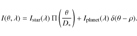
|
(1) |
We indicate by
The plane of spatial frequency, defined by the vector
![]() ,
is covered by a single-baseline interferometer and the u-axis vector is chosen along the interferometric baseline vector
,
is covered by a single-baseline interferometer and the u-axis vector is chosen along the interferometric baseline vector ![]() (with
(with
![]() ). The Fourier transform
). The Fourier transform
![]() of the brightness distribution in this plane is
of the brightness distribution in this plane is
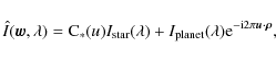
|
(2) |
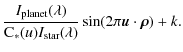
where C*(u) (or identically C
| |
![$\displaystyle 1-\frac{I_{\rm planet}(\lambda)}{{\rm C}_*(u)I_{\rm star}(\lambda)}\:\left[1-\frac{1}{2}\cos(2\pi {\vec u}\cdot{\vec \rho})\right]$](/articles/aa/full_html/2010/07/aa13142-09/img30.png)
|
(3) | |
|
(4) |
As the phase cannot be measured without any reference, we use the possibility offered by both MIDI and AMBER instruments to measure the relative phase between each of the channels of the spectrally dispersed fringes. The reference phase is usually taken as the average phase over all the channels. Then this gives access to the colour-differential phase, without the unknown constant k that disappears in the colour difference. The same process can be followed for obtaining the differential visibility.
In principle, the visibility and the phase carry complementary physical information, and both might be used for detecting and characterizing extrasolar planets. The fundamental noise sources affect the differential visibility and phase in a similar way, in contrast to the dispersion effects. The variations in the achromatic and chromatic OPD terms are more easily calibrated using the phase, since it has a linear dependence on OPD. This is not the case for visibility that has a quadratic dependence and is consequently much less affected, especially in differential mode. This constitutes a disadvantage since we want to estimate the amplitude of the dispersion effects on the OPD. A consequence is that some particular calibration tools allow us to correct the AMBER phase from systematic instrumental effects and not the visibility (Vannier et al. 2006). The closure phase could be also considered in parallel and would provide an observable that is free of any atmospheric and dispersion effects; however, it is not available for a two-telescope interferometer such as MIDI, so we instead focus on the differential phase.
2.3 Assumptions on the astrophysical source
The modelling of the flux of an irradiated planet requires careful attention on the radiative transfer conditions related to the stellar irradiation. Adressing this issue, Barman et al. (2001) modelled cool and hot irradiated 1-Jupiter mass and radius EGPs with intrinsic temperatures of 500 K and 1000 K, and various orbital distances. Regarding the atmospheric composition, especially in terms of opacity, two types of atmosphere were considered: a ``dusty'' atmosphere where all the particles and grains (mainly silicates) remain in the upper atmosphere, and a ``condensed'' one where dust has been removed from the upper atmosphere by condensation and gravitational settling. In order to conveniently model the Gliese 86b spectrum, different physical assumptions have to be considered.
The intrinsic temperature is the first discriminating parameter of the synthetic spectra. Because Gliese 86 is a few billion years old main-sequence star, its planetary companion can be considered as a fairly old planet that has undergone significant intrinsic cooling since its formation, regardless of any stellar irradiation (Guillot et al. 1996). Thus, an intrinsic temperature of 500 K seems more relevant for modelling Gliese 86b. Since we address the case of an irradiated planet, the atmosphere type and the opacity sources are essential and constitutes the second discriminating parameter. For our concern, we considered only the ``condensed'' model of Barman et al. (2001) since it seems more realistic for the substellar objects of weak temperature than the ``dusty'' one (Chabrier & Baraffe 2000).
Because it is required for calculating the theroretical planetary flux
received on Earth, the issue of the planetary radius has to be
carefully addressed in the irradiated case. According to theory (Saumon et al. 1996),
isolated extrasolar giant planets shrink rapidly. In contrast, at small
orbital separations, the evolution of an irradiated planet and of its
radius are substantially slowed down by stellar heating (Burrows et al. 2000; Guillot et al. 1996).
Therefore, to determine the theoretical radius of Gliese 86b, we
used a mass-radius relation for irradiated planets, obtained from Guillot (2005).
It considered various parameters involved in the definition of the
cooling timescale and the temperature profile of the atmosphere. These
parameters include the 1-bar temperature, the atmospheric composition,
the opacity sources and the presence of clouds. Considering a 1-bar
temperature of 1500 K for Gliese 86b, according to the
theoretical values found in Barman et al. (2001), and a mass ranging from 4 to 13
![]() ,
the corresponding radius of Gliese 86b would range from 1.05 to 1.2
,
the corresponding radius of Gliese 86b would range from 1.05 to 1.2
![]() .
.
![\begin{figure}
\par\includegraphics[height=60mm,width=77mm,clip]{13142fg2.eps}
\end{figure}](/articles/aa/full_html/2010/07/aa13142-09/img35.png)
|
Figure 2:
Mean phase amplitude produced by Gliese 86b over the N band as a function of different values of baseline projected onto the separation vector |
| Open with DEXTER | |
From an updated version of the 2001 synthetic spectra, Barman
(private communication) has thus provided us with a synthetic spectrum
of Gliese 86b following the physical assumptions described above,
and the orbital features already determined by radial velocimetry.
Since this synthetic spectrum corresponds to the flux at the surface of
the planet, we needed to scale it by a dilution factor, implying the
planetary radius, for getting
![]() .
A range of radii wider than the theoretical assumptions, from 1 to
.
A range of radii wider than the theoretical assumptions, from 1 to
![]() ,
has been considered here. Concerning
,
has been considered here. Concerning
![]() ,
a simple blackbody law of emission was used with the effective
temperature of Gliese 86, which we considered to be equal to about
5200 K (Butler et al. 2006; Flynn & Morell 1997).
,
a simple blackbody law of emission was used with the effective
temperature of Gliese 86, which we considered to be equal to about
5200 K (Butler et al. 2006; Flynn & Morell 1997).
2.4 Geometric parameters and resulting phase signal
Given that Gliese 86b was discovered by radial velocimetry, the
inclination and position angles of the binary system in the plane of
the sky are unknown. As a consequence, in the expression of the
theoretical phase, the value of the projected baseline
![]() resulting from the scalar product
resulting from the scalar product
![]() is also unknown. We thus consider a wide range of projected baselines from 10 to 130 m to calculate the theoretical signal.
is also unknown. We thus consider a wide range of projected baselines from 10 to 130 m to calculate the theoretical signal.
As an example, the interferometric phase is calculated in Fig. 1
for a projected baseline value of 110 m (assuming a 130 m
baseline at ground level) and for a mean planetary radius equal to
1.2
![]() .
We see that in N band (8 to 13
.
We see that in N band (8 to 13 ![]() m),
the signal is quite linear because of the partially resolved separation
between star and planet, and its corresponding amplitude is close to 0.1
m),
the signal is quite linear because of the partially resolved separation
between star and planet, and its corresponding amplitude is close to 0.1![]() .
The ``phase amplitude'' is defined as the difference between the highest and lowest values over the N band of the interferometric phase.
.
The ``phase amplitude'' is defined as the difference between the highest and lowest values over the N band of the interferometric phase.
In Fig. 2, the evolution of the phase amplitude over the N band is displayed as a function of the projected baseline.
It appears that for most values of projected baseline, the mean phase amplitude is greater than 0.05![]() .
In addition, the maximum phase amplitude, equal on average to 0.9
.
In addition, the maximum phase amplitude, equal on average to 0.9![]() ,
does not occur for the 130 m baseline but instead for the shorter
90 m baseline. The reason is that, while large projected baseline
values imply normally large phase amplitude because of the higher
angular resolution, the phase amplitude also depends on the evolution
of the sine modulation period as a function of wavelength (see
Eq. (4)).
A 0.05
,
does not occur for the 130 m baseline but instead for the shorter
90 m baseline. The reason is that, while large projected baseline
values imply normally large phase amplitude because of the higher
angular resolution, the phase amplitude also depends on the evolution
of the sine modulation period as a function of wavelength (see
Eq. (4)).
A 0.05![]() level
of precision on the phase measurement would allow us to achieve the
phase signal of the planet for a large set of projected baseline
values, ranging from 50 to 130 m.
level
of precision on the phase measurement would allow us to achieve the
phase signal of the planet for a large set of projected baseline
values, ranging from 50 to 130 m.
3 Dispersion and correction of the phase signal
3.1 Effects of dispersion
The incoming wavefronts collected by each telescope are affected by different pertubations during their propagation through the atmosphere and the instrument. Most of the perturbations affecting independently each wavefront are corrected by an adaptive optics device. Then for single mode spatial-filtered instrument such as MIDI, the residual wavefront perturbations are eventually limited to an optical path difference (OPD) between the two beams. This implies a degradation of the interferometric observables and especially the phase, since a perturbating term is added to the intrinsic phase signature of the science source. The causes producing such a pertubating OPD are
- use of the air-filled delay lines to correct an astronomical differential path delay occurring in the vacuum, a contribution that can be seen as a quasi-static OPD component.
- other causes such as the refractive index fluctuations of free atmosphere and air inside interferometric tunnels, a contribution that can be seen as a variable OPD component as a function of time.
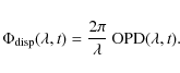
|
(5) |
The dispersion relations and their effect on stellar interferometry can be found under a detailed form in Tango (1990) and Davis et al. (1998). To address the problem of the dispersion caused by the air, the atmospheric refractivity included in the expression of the OPD can be written as a sum over atmospheric constituents by approximating the Lorentz-Lorenz relation, to yield
|
(6) |
where
| (7) |
which yields
|
(8) |
According to the first paragraph of this section, an OPD term is caused either by a geometric path difference (quasi-static contribution) or by a refractive index fluctuation (variable contribution). Considering water vapour, the general expression expliciting these contributions is
| |
= | ||
| = | (9) |
The expression is the same for dry air. The ``quasi-static'' contribution corresponds to the common situation where an astrophysical object is observed at a projected zenith distance
The ``variable'' contribution highlights that, even though both beams
cover an equal geometrical path from the top of the atmosphere to the
recombining device (
![]() ), differential density fluctuations of the atmospheric component between each path,
), differential density fluctuations of the atmospheric component between each path,
![]() ,
will introduce an OPD. These fluctuations depend on the temperature,
pressure, and humidity differences between the paths of the beams,
consequently on time.
,
will introduce an OPD. These fluctuations depend on the temperature,
pressure, and humidity differences between the paths of the beams,
consequently on time.
The terms
![]() and
and
![]() contain
a dominant achromatic term corresponding to the uncorrected achromatic
delay or ``piston'' between beams, and a chromatic term representing
the higher order dispersion. The piston is equal to the mean slope of
the linear component of the phase as a function of the wavenumber
contain
a dominant achromatic term corresponding to the uncorrected achromatic
delay or ``piston'' between beams, and a chromatic term representing
the higher order dispersion. The piston is equal to the mean slope of
the linear component of the phase as a function of the wavenumber
![]() .
In mathematical terms, this piston corresponds to the zero-order term of
.
In mathematical terms, this piston corresponds to the zero-order term of
![]() ,
that is to say, the group delay as defined in Meisner & Le Poole (2003) or Colavita et al. (2004).
This linear part of the ``dispersive'' phase will affect the
measurements by adding to the linear part of the planetary signal.
,
that is to say, the group delay as defined in Meisner & Le Poole (2003) or Colavita et al. (2004).
This linear part of the ``dispersive'' phase will affect the
measurements by adding to the linear part of the planetary signal.
By explicitly calculating the ``achromatic'' and ``chromatic''
dispersion terms for each atmospheric component, the total dispersive
phase can be formulated as
| |
= | ||
| (10) |
Here,
In terms of data processing, where the different contributions
producing a dispersive phase are generally removed by a fitting
procedure, it is convenient to make
![]() and
and
![]() explicit as a function of one single parameter,
explicit as a function of one single parameter,
![]() and
and
![]() respectively, containing all the contributions that affects the dispersion amplitude:
respectively, containing all the contributions that affects the dispersion amplitude:
| |
= | ||
| = | (11) |
The behaviour of dry and humid refractivity laws is different according the spectral band. The empirical humid law is very sloping in the mid-infrared and very flat in the near infrared, whereas it is the opposite for the theoretical dry air law. Therefore in the N band, the dispersion introduced by the propagation through the air is dominated by its humid component (Meisner et al. 2004; Meisner & Le Poole 2003), and the dispersive phase affecting the MIDI data becomes
|
(12) |
Other terms affect the interferometric phase measurements, such as the fundamental noise or the instrumental phase. They are discussed in the following section.
3.2 Mono-band observations
In mono-band interferometric observations, the correction of the
different terms of the dispersive phase is performed by fitting the
measured interferometric phase over the spectral range of the band with
refractive index models of dry air and water vapour.
The first contribution of the dispersive phase to be removed from
measurements is the dominant linear part. A linear fit on the total
interferometric phase is performed to estimate and remove the mean
slope, that is to say, the ``![]() '' term detailed in Sect. 3.1.
Unfortunately, by doing so, we also remove any linear trend due to the planet signal.
'' term detailed in Sect. 3.1.
Unfortunately, by doing so, we also remove any linear trend due to the planet signal.
Once this contribution has been removed, the phase is constituted by
the non-linear contribution of the dispersion along with the remaining
planet signal, both having a curvature-like or quadratic aspect. The
amplitude of the curvature introduced by the non-linear dispersion term
can typically reach about 10![]() (Meisner et al. 2004) and overwhelm the curvature due to the planet.
For the sake of detection, an additional correction is thus required.
(Meisner et al. 2004) and overwhelm the curvature due to the planet.
For the sake of detection, an additional correction is thus required.
A fit of the phase curvature, by estimating
![]() and
and
![]() from a model of refractivity, would allow removal of the 2nd order
contribution of the dispersive phase. However, the curvature-like part
of the planetary signal would be removed at the same time, letting an
even smaller phase signature from the planet.
from a model of refractivity, would allow removal of the 2nd order
contribution of the dispersive phase. However, the curvature-like part
of the planetary signal would be removed at the same time, letting an
even smaller phase signature from the planet.
As previously mentioned, two other terms affect the
differential phase measurements, the instrumental and fundamental noise
terms. For MIDI, the instrumental term can in principle be calibrated
by a nearby star observed close in time to the target star. A device
called BCD (for beam commutator device) allows us to quickly and
accurately calibrate the instrumental phase of AMBER. Concerning the
fundamental noises, they represent the sources of noise that cannot be
reduced for a given instrumental setup. In the N band,
where the thermal background is the principal source of fundamental
noise, an empirical law gives the expected value for the relative error
on phase assuming that MIDI is used with photometric channels:

|
(13) |
with
3.3 Multi-band observations
For astrophysical sources such as close-in EGPs, the differential phase has a strong chromatic dependence. The exoplanet signature may be negligible, that is, below the fundamental noise level in one spectral band and significant in another band. A ``multi-band'' approach is thus applicable to correct the water vapour dispersion. Colavita et al. (2004) addresses this issue in the context of the standard phase referencing. By using a phase reference in K band, they estimate that 59% of the water vapour's seeing effects would remain uncompensated in N band, because of the higher chromatic ``sensitivity'' of the humid dispersion law. However, these results do not apply to our approach in which fringes were independently and simultaneously obtained in both bands. As explained, the ``reference phase'' in K band is not used here as a first-order tracking of the fringes in N band (science band), but rather as an estimate of the instantaneous amplitude of the water vapour dispersion.
In a single band observation, we saw that the estimation of the
dispersion effects takes not only the ``true'' amplitude of dispersion
into account, but also the ``dispersion-like'' part of the planetary
signal. In contrast, by simultaneously observing in a band where the
astrophysical signal is negligible, we should be able to directly
estimate the true amplitudes of dispersion represented by the
achromatic factors,
![]() and
and
![]() ,
without any additional significative phase signal coming from the
source. Then an extrapolation of these achromatic factors to the
spectral band of interest would allow correction of only the non-linear
dispersive component of the phase without affecting the remaining
object signal.
,
without any additional significative phase signal coming from the
source. Then an extrapolation of these achromatic factors to the
spectral band of interest would allow correction of only the non-linear
dispersive component of the phase without affecting the remaining
object signal.
In our case, that is MIDI observing in N band and AMBER observing in K band, the parameter of interest to extrapolate is
![]() .
Nevertheless, the precision on the estimates of this parameter depends
on the data quality, and in some cases a degeneracy between
.
Nevertheless, the precision on the estimates of this parameter depends
on the data quality, and in some cases a degeneracy between
![]() and
and
![]() may occur in the fit. In a general way, if the differential phase in K band
is degraded and deviates from the typical water vapour dispersion
pattern, the estimation of the achromatic factor representing the
dispersion amplitude is affected by an error denoted hereafter as
may occur in the fit. In a general way, if the differential phase in K band
is degraded and deviates from the typical water vapour dispersion
pattern, the estimation of the achromatic factor representing the
dispersion amplitude is affected by an error denoted hereafter as
![]() .
According to Eq. (12) and assuming that the linear part has been
removed, the corresponding error on the estimation of the de-pistoned
dispersive phase affecting the other band is
.
According to Eq. (12) and assuming that the linear part has been
removed, the corresponding error on the estimation of the de-pistoned
dispersive phase affecting the other band is
|
(14) |
More precisely, this expression corresponds to the accuracy with which the N band differential phase could be corrected from the 2nd order water vapour dispersion, using the parameter
In parallel, we compared the relative slopes of the tabulated water vapour dispersion law on the extent of the K and N band, as shown in Colavita et al. (2004) or Mathar (2004). The chromatic sensitivity of the water vapour refractivity appears to be two times greater in N band than in K band. It thus implies that, for a same dispersion amplitude
![]() ,
the corresponding curvature of the de-pistoned dispersive phase is about two times greater in N than in K band. Therefore, it is essential to get precise differential phase measurements in K band, hence precise measurements of
,
the corresponding curvature of the de-pistoned dispersive phase is about two times greater in N than in K band. Therefore, it is essential to get precise differential phase measurements in K band, hence precise measurements of
![]() ,
in order to limit the propagation of the error when applying this achromatic factor to the N band.
,
in order to limit the propagation of the error when applying this achromatic factor to the N band.
For example, we plotted in Fig. 3 the relative error on the wet dispersion parameter
![]() with respect to the standard deviation, per spectral channel, of a
Gaussian error that would affect a dispersive phase calculated from a
standard humid dispersion law in K band (in radians). According to the grey curve in Fig. 3, this shows that a typical error of 0.01 radians on the phase measurement in K band
implies a relative error of 5% on the wet dispersion parameter.
According to Eq. (14), if the water vapour dispersion introduces,
for example, a curvature amplitude of 5
with respect to the standard deviation, per spectral channel, of a
Gaussian error that would affect a dispersive phase calculated from a
standard humid dispersion law in K band (in radians). According to the grey curve in Fig. 3, this shows that a typical error of 0.01 radians on the phase measurement in K band
implies a relative error of 5% on the wet dispersion parameter.
According to Eq. (14), if the water vapour dispersion introduces,
for example, a curvature amplitude of 5![]() in N band, the calibration accuracy would be
in N band, the calibration accuracy would be
![]() .
With such a corrected N band differential phase, we would stand at a factor of about 10 above the phase signal of Gliese 86b.
.
With such a corrected N band differential phase, we would stand at a factor of about 10 above the phase signal of Gliese 86b.
![\begin{figure}
\par\includegraphics[height=62mm,width=8.3cm,clip]{13142fg3.eps}
\end{figure}](/articles/aa/full_html/2010/07/aa13142-09/img80.png)
|
Figure 3: Relative error on wet dispersion parameter (black: average; grey: rms) as a function of a Gaussian error per spectral channel affecting a theoretical dispersive phase in K band. The error on the K band phase is expressed in radians, and 12 spectral channels are considered. |
| Open with DEXTER | |
3.4 Actual required level of precision
![\begin{figure}
\par\includegraphics[height=59mm,width=83mm,clip]{13142fg4.eps}
\end{figure}](/articles/aa/full_html/2010/07/aa13142-09/img81.png)
|
Figure 4:
Example of the expected amplitude of the planet signal as a function of wavenumber (k) in N band. In this example, we consider a projected baseline of 110 m, and a planetary radius of 1.2
|
| Open with DEXTER | |
As discussed in Sect. 3.2, the first-order correction of dispersion effects will remove any linear contribution in the interferometric phase, which also includes the linear part of the object phase. Therefore the actual phase amplitude has to be evaluated on an ``de-pistoned'' interferometric phase.
In the case of a 110 m baseline and a
![]() planetary radius, we see in Fig. 4
that the remaining planetary phase signal (or ``de-pistoned'' phase) is
a curvature-like function of the wavelength (or wavenumber) in N-band. The amplitude of this signal is consequently lower and approximately equal to 0.03
planetary radius, we see in Fig. 4
that the remaining planetary phase signal (or ``de-pistoned'' phase) is
a curvature-like function of the wavelength (or wavenumber) in N-band. The amplitude of this signal is consequently lower and approximately equal to 0.03![]() instead of 0.08
instead of 0.08![]() .
.
In Fig. 5, we represent the evolution of the amplitude of the ``de-pistoned'' phase over the N band as a function of the projected baseline.
The curvature substantially varies with the projected baseline and is at its maximum for the 130 m baseline (![]() 0.05
0.05![]() ), whereas it is close to zero for projected baselines lower than 70 m where the phase has a strong linear trend.
), whereas it is close to zero for projected baselines lower than 70 m where the phase has a strong linear trend.
![\begin{figure}
\par\includegraphics[height=58mm,width=77mm,clip]{13142fg5.eps}
\end{figure}](/articles/aa/full_html/2010/07/aa13142-09/img83.png)
|
Figure 5:
Amplitude of the ``de-pistoned'' Gliese 86b interferometric phase over the N band as a function of different values of baseline projected onto the separation vector |
| Open with DEXTER | |
4 Experience
4.1 Technical scheme of simultaneous observations
For the first time, the instruments MIDI (in the N-band,
![]() m) and AMBER (in the near-IR
m) and AMBER (in the near-IR
![]() m) were simultaneously used for
the observation of Gliese 86.
In Fig. 6,
we represent the simplified optical path of AMBER and MIDI in the VLTI
laboratory.
We chose to set MIDI as the
master instrument for the VLTI subsystems, while AMBER was running in a
stand-alone mode. The simultaneous use of the two instruments implies,
in principle, that they have similar transversal alignment,
longitudinal alignment, and temporal synchronicity. In practice, each
of these adjustments has only been approximated, as best as possible.
m) were simultaneously used for
the observation of Gliese 86.
In Fig. 6,
we represent the simplified optical path of AMBER and MIDI in the VLTI
laboratory.
We chose to set MIDI as the
master instrument for the VLTI subsystems, while AMBER was running in a
stand-alone mode. The simultaneous use of the two instruments implies,
in principle, that they have similar transversal alignment,
longitudinal alignment, and temporal synchronicity. In practice, each
of these adjustments has only been approximated, as best as possible.
![\begin{figure}
\par\includegraphics[height=63mm,width=84mm,clip]{13142fg6.eps}
\end{figure}](/articles/aa/full_html/2010/07/aa13142-09/img86.png)
|
Figure 6: Simplified optical path of AMBER and MIDI in the VLTI laboratory, highlighting the important elements to be considered for parallel operation. |
| Open with DEXTER | |
Table 1: Log of the observing sequences (left table: November 17 2007; right table: November 24 2007).
Because AMBER is more stringent in terms of transversal alignment
(because of the shorter wavelength and the use of a fiber spatial
filter), the global pointing offsets used for that alignment were found
by optimizing the fiber injection on AMBER. Due to a slight
non-alignment between the two instruments, this optimization on AMBER
resulted for MIDI in a 2-pixel shift in the telescopes beam overlap,
although the standard tolerance for the overlap shift is in principle
0.8 pixels. Nevertheless, the overlap quality was still good
enough to produce fringes with the aim of measuring differential phases
on the target (1-Jy at 12 ![]() m correlated flux). Moreover, this misalignment prevented us from extracting well-calibrated visibility curves.
m correlated flux). Moreover, this misalignment prevented us from extracting well-calibrated visibility curves.
For the longitudinal alignment, the fringe optimization was also first
performed on AMBER, by moving the external VLTI delay lines. It
was then necessary to correct the optical path difference offset
between AMBER and MIDI (measured on a bright target at the beginning
of each night before the observations) by moving the internal delay
lines of MIDI up to a value
![]() corresponding to the fringe
optimization of MIDI. During the observation, the fringe tracking was performed by MIDI, which can send corrections to
the VLTI OPD controller. Therefore the fringes were not stabilized on AMBER, with a residual OPD of about
corresponding to the fringe
optimization of MIDI. During the observation, the fringe tracking was performed by MIDI, which can send corrections to
the VLTI OPD controller. Therefore the fringes were not stabilized on AMBER, with a residual OPD of about ![]() m.
As FINITO was not
used, the expected data quality of AMBER was the one obtained when
AMBER works alone with a correct estimation of the baseline
vector and under good seeing. The main limitation of this longitudinal
alignment procedure was the chromatic dependence of the OPD offset
m.
As FINITO was not
used, the expected data quality of AMBER was the one obtained when
AMBER works alone with a correct estimation of the baseline
vector and under good seeing. The main limitation of this longitudinal
alignment procedure was the chromatic dependence of the OPD offset
![]() .
As a result of that effect, the AMBER fringes, initially positioned
vertically, started to be significantly tilted after a few hours of
observation (i.e. when the change in the projected baseline of the
target induced a significant differential OPD in K band).
.
As a result of that effect, the AMBER fringes, initially positioned
vertically, started to be significantly tilted after a few hours of
observation (i.e. when the change in the projected baseline of the
target induced a significant differential OPD in K band).
4.2 Sequence of the observations
These simultaneous observations were carried out on 2007 November 17 and 24 with the UT1-UT4 baseline during five hours (from 00:00 UT to 04:30 UT, approximately). According to the predicted ephemerides of the system, this interval of one week would correspond to both maxima for the angular separation between star and planet, putting the planet on one side of the star and then on the other.
Moreover, we tried to observe close to the plane perpendicular to the baseline (plane corresponding to the zero delay position of the delay lines) in order to minimize the air asymmetry into the interferometric tunnels as much as possible. Also, the observation of the source at opposite positions before and after the zero delay crossing could be used for calibrating the chromatic dispersion within the delay lines using only MIDI. The consequent switch of the OPD sign would imply an inversion of the slope of the differential phases measured at opposite positions before and after the zero delay crossing. Then a simple subtraction would allow removal of the dispersive contribution due to the air asymmetry within the delay lines. If the amplitude of the atmospheric dispersion is greater than the contribution of the dispersion within the delay lines, this method is no longer usable. Moreover, this method requires very good timing on the observing sequence.
In order to test this possibility of calibration, in addition to the main calibration procedure using AMBER and MIDI, we considered it in the preparation of the observing sequence of each night. The zero delay crossing and the use of the consequent switch of the OPD sign were attempted for the target and two calibrators, HD 9362 and HD 12524, which were observed alternately as shown in Table 1. Unfortunately, some problems of coordinates and proper motion correction for Gliese 86 disordered the prepared observing sequence for both nights, during the telescope pointing and the acquisition on IRIS.
Despite all of that, fringes were detected for the three objects. For example, concerning the ``master'' instrument MIDI, for the first night, nine fringe exposures were obtained for Gliese 86, seven for HD 9362, and three for HD 12524. For the second one, we also did nine fringe exposures for Gliese 86, four for HD 9362, and two for HD 12524.
However, because of the changes in the prepared observing sequences, we were only able to observe the first calibrator (HD 9362) before and after the zero delay crossing. Although the slope inversion due to the switch of the OPD sign was visible for two opposite phase measurements, the method was not really usable given the greater amplitude of the atmospheric dispersion during most of the observations and given the disordered observing sequence.
5 Results
5.1 Precision reached on the extrapolation with AMBER data
The simultaneous observation with the two VLTI instruments was a success and fringes were obtained with AMBER while MIDI was guiding. Due to technical compromizes for the longitudinal alignment, the MIDI data were degraded giving a non-optimum quality and a poor SNR on the differential phase.
![\begin{figure}
\par\includegraphics[height=67mm,width=84mm,clip]{13142fg7.eps}
\end{figure}](/articles/aa/full_html/2010/07/aa13142-09/img91.png)
|
Figure 7: Differential phases of Gliese 86 observed with AMBER on 2007 November 17, for a time sequence of about 12 min. Each curve corresponds to a phase that is auto-calibrated from instrumental internal effects using the BCD, and the average slope is subtracted. |
| Open with DEXTER | |
The quality of the fringes observed with AMBER varies largely depending on the observing conditions and on the quality of the beam injection. In Fig. 7, we present the differential phases from a ``good'' sequence, after de-pistoning and subtraction of internal instrumental effects using an autocalibration by a BCD. The statistical dispersion between the curves over that 12 min sequence is about 1 degree rms, on average. The plot shows a fairly stable rough pattern, which is even more obvious when looking at the residual after fitting the phase curves individually with the wet and dry chromatic dispersion laws (Fig. 8). The fit residuals are roughly stationary and show a statistical dispersion of about 0.4 degree rms that is compatible with a normal distribution around the average curve. The average pattern, showing sine-like waves, is believed to originate from a parasitic Fabry-Perot effect in the AMBER polarizers (replaced since). An additional piston effect probably affected the AMBER observations, whose quality is significantly poorer in other sequences, since the tracking of AMBER fringes was performed with MIDI without using FINITO. Fringes were not stabilized by the fringe tracking of MIDI, and this is particularly sensitive because of the UTs.
![\begin{figure}
\par\includegraphics[height=67mm,width=84mm,clip]{13142fg8.eps}
\end{figure}](/articles/aa/full_html/2010/07/aa13142-09/img92.png)
|
Figure 8: Residual of the AMBER differential phases presented in Fig. 7 after individual fits of the wet and dry chromatic dispersion laws. |
| Open with DEXTER | |
From Monte-Carlo simulations of the fit of noisy simulated data, we
previously deduced a relationship between the precision on the
retrieved dispersion parameters and the standard deviation in the noise
on the differential phase. The observed scatter on the AMBER residual
phase presented in Fig. 8,
whose statistics are consistent with our simulations, can then be
related to a relative error on the wet dispersion parameter. For the
sequence presented above, that error is about ![]() .
.
According to Eq. (14) and knowing that
![]() ,
we can deduce the correction accuracy of the dispersive phase affecting the MIDI data, namely
,
we can deduce the correction accuracy of the dispersive phase affecting the MIDI data, namely
![]() .
For that we evaluate the amplitude of
.
For that we evaluate the amplitude of
![]() ,
which is the curvature amplitude affecting the MIDI differential phases
during the same sequence as the one considered for AMBER.
Unfortunately, because of the strong loss of SNR affecting the MIDI
data, the differential phases of Gliese 86 obtained during this
observing sequence were too noisy to clearly distinguish the typical
curvature-like wet dispersion pattern. Instead, we used the first phase
measurement of the second bright calibrator HD 12524, obtained
just after the end of the first observing sequence of Gliese 86.
At this time, both objects were observed with similar airmasses and
,
which is the curvature amplitude affecting the MIDI differential phases
during the same sequence as the one considered for AMBER.
Unfortunately, because of the strong loss of SNR affecting the MIDI
data, the differential phases of Gliese 86 obtained during this
observing sequence were too noisy to clearly distinguish the typical
curvature-like wet dispersion pattern. Instead, we used the first phase
measurement of the second bright calibrator HD 12524, obtained
just after the end of the first observing sequence of Gliese 86.
At this time, both objects were observed with similar airmasses and
![]() values (see Fig. 1),
therefore the curvature observed on the differential phase of
HD 12524 should give a fairly good estimation of the amplitude of
the dispersive phase that affected the first sequence of Gliese 86
phase measurements.
values (see Fig. 1),
therefore the curvature observed on the differential phase of
HD 12524 should give a fairly good estimation of the amplitude of
the dispersive phase that affected the first sequence of Gliese 86
phase measurements.
By fitting the differential phase of HD 12524 with the tabulated water vapour dispersion law taken from Mathar (2004), we estimated a curvature amplitude of about 13![]() ,
which gives
,
which gives
![]()
![]() .
With such a calibration accuracy for MIDI differential phases, we
finally arrive at a factor of 10 above the phase signature from the
planet Gliese 86b (
.
With such a calibration accuracy for MIDI differential phases, we
finally arrive at a factor of 10 above the phase signature from the
planet Gliese 86b (![]() 0.03
0.03![]() ).
).
5.2 Precision reached on MIDI curvature measurements
As discussed above, the phase signature from Gliese 86b is about 0.03Because the AMBER data is unusable for the extrapolation and correction of the wet dispersion, we focus on the possibility of estimating the level of precision of the curvature measurement that we could achieve with the MIDI data. This can be done by correcting the instrumental and atmospheric effects as much as possible on the phases of a calibrator and after estimating a curvature on the residual phases. The reason is that a calibrator is generally an unresolved star with an intrinsic phase equal to zero.
In our case we considered the data of the calibrator HD 9362 taken during the first night. The estimation of the standard deviation of the curvature measurements between the phases of various exposures (7 for HD 9362) can give the general precision that we could achieve.
The method of estimation consists in several steps:
- The mean of all the measured differential phases is subtracted from
each differential phase (produced by each fringe exposure) noted
 :
:
(15)
The data reduction software that we used here, named EWS, allows us to check that phases are not wrapped (Jaffe 2004). This calibration removes a large part of phase trends that could be caused by instrumental and other invariable effects during the night, such as a large part of the ozone absorption signature at 9.6 m.
m.
- Then we use the refractive index model of Mathar to fit and
remove the variable water vapour dispersion not suppressed by the first
step:
(16)
From that point, the residual noise only remains in the curvature of the phase. - A 2nd order polynomial fit is applied to each of the residual phases (
 )
for revealing the residual curvature.
)
for revealing the residual curvature.
- The residual curvature can be directly estimated by
calculating the second difference between three values of the
polynomial fit for each exposure: at 8 m, at a wavelength located around the middle of the band, and at 13 m. We note these values S8,
 ,
and S13, such that the second difference is
,
and S13, such that the second difference is
(17)
It is important to note that we maximize the curvature estimation here since the wavelength corresponding to
is chosen precisely to maximize the second difference.
![\begin{figure}
\par\includegraphics[height=60mm,width=83mm,clip]{13142fg9.eps}
\end{figure}](/articles/aa/full_html/2010/07/aa13142-09/img105.png)
|
Figure 9: Evolution of the estimated phase curvature for the calibrator HD 9362 as a function of the considered spectrum (or set of data). The number on the x-axis, giving the set of data, corresponds to the chronological order of measurements during the night. |
| Open with DEXTER | |
This estimation of the dispersion of the second difference during the
night means that we could not measure a curvature smaller than
![]() .
This value stands at a factor 10 above the phase signal of Gliese 86b.
.
This value stands at a factor 10 above the phase signal of Gliese 86b.
6 Discussion and future improvements
Direct observation of close-in EGPs is currently one of the most
challenging programmes for the MIDI instrument, the VLTI, and in
general for ground-based long baseline interferometry. By considering
the observing and data reduction process, a theoretical precision of
the order of 0.03![]() on the phase would be required to detect the exoplanet Gliese 86b
orbiting the K-dwarf star Gliese 86. From the data of our MIDI GTO
observations of 2007 November, we estimated the smallest measurable
curvature as equal to 0.33
on the phase would be required to detect the exoplanet Gliese 86b
orbiting the K-dwarf star Gliese 86. From the data of our MIDI GTO
observations of 2007 November, we estimated the smallest measurable
curvature as equal to 0.33![]() .
This value is still ten times higher than the theoretical requirements.
.
This value is still ten times higher than the theoretical requirements.
As a step towards potential detection, a more favourable source providing a stronger signal could become available since new targets have been discovered by radial velocimetry. In this case, a better resolved and, at the same time a warmer planet would be appropriate. Thanks to better resolution, we would have an almost complete sine modulation cycle all over the whole N band (see Fig. 1) and no longer a quasi-linear phase. It would thus imply a larger remaining phase amplitude due to the planet, after suppression of the piston.
In addition to the feasibility study accompanying this first attempt, we have shown that it is possible to carry out parallel observations of the same target with AMBER and MIDI. By using the fringes obtained in K-band, the aim was to correct the phase in N-band from the strong water vapour dispersion without removing the planet contribution. However, several technical constraints and problems degraded the AMBER data, so they were too noisy to be directly extrapolated. Nevertheless, in terms of calibration accuracy, we can infer that we approximately stand at a factor of 10 above the phase signature from the planet.
Different technical and observational improvements were made (two first items in the list) or could be envisaged to get better data quality for both instruments, consequently improving the chances of detection:
- Ability of AMBER to control its ACUs (atmospheric compensation units) in order to optimize the injected flux with the IRIS instrument offsets set for MIDI. Thanks to that the MIDI overlap will be much better for our experiment;
- Use of FINITO and fix of the polarizers on AMBER to obtain stabilized fringes on this instrument;
- Implementation of slight modifications in the AMBER and MIDI template sequence files (perspective of an AMBER+MIDI service mode) including the synchronization of the frames of MIDI and AMBER, and an automatic correction of the delay lines position at each preset;
- Use of a larger baseline to increase the angular resolution;
- Correction of the ozone absorption signature in the phase by the data reduction process.
We would like to thank the ESO staff of Paranal and Garching, especially Thomas Rivinius, Markus Schoeller, and Fredrik Rantakyro, for their collaboration that made this experiment possible. We also thank Travis Barman, from the Lowell observatory, for providing us with an updated synthetic spectrum corresponding to the Gliese 86b characteristics, along with the referee for his valuable comments that improved the paper.
References
- Barman, T. S., Hauschildt, P. H., & Allard, F. 2001, ApJ, 556, 885 [NASA ADS] [CrossRef] [Google Scholar]
- Burrows, A., Guillot, T., Hubbard, W. B., et al. 2000, ApJ, 534, L97 [NASA ADS] [CrossRef] [PubMed] [Google Scholar]
- Butler, R. P., Wright, J. T., Marcy, G. W., et al. 2006, ApJ, 646, 505 [NASA ADS] [CrossRef] [Google Scholar]
- Chabrier, G., & Baraffe, I. 2000, ARA&A, 38, 337 [NASA ADS] [CrossRef] [Google Scholar]
- Colavita, M. M., Swain, M. R., Akeson, R. L., Koresko, C. D., & Hill, R. J. 2004, PASP, 116, 876 [NASA ADS] [CrossRef] [Google Scholar]
- Davis, J., Tango, W. J., & Thorvaldson, E. D. 1998, AO, 37, 5132 [CrossRef] [Google Scholar]
- Flynn, C., & Morell, O. 1997, MNRAS, 286, 617 [NASA ADS] [CrossRef] [Google Scholar]
- Guillot, T. 2005, Annual Review of Earth and Planetary Sciences, 33, 493 [Google Scholar]
- Guillot, T., Burrows, A., Hubbard, W. B., Lunine, J. I., & Saumon, D. 1996, ApJ, 459, L35 [NASA ADS] [CrossRef] [Google Scholar]
- Jaffe, W. J. 2004, in New Frontiers in Stellar Interferometry, ed. W. A. Traub, SPIE Conf., 5491, 715 [Google Scholar]
- Joergens, V., & Quirrenbach, A. 2004, in SPIE Conf. Ser. 5491, ed. W. A. Traub, 551 [Google Scholar]
- Leinert, C., Graser, U., Przygodda, F., et al. 2003, ApSS, 286, 73 [Google Scholar]
- Lopez, B., Petrov, R. G., & Vannier, M. 2000, in SPIE Conf. Ser. 4006, ed. P. Léna, & A. Quirrenbach, 407 [Google Scholar]
- Mathar, R. J. 2004, AO, 43, 928 [Google Scholar]
- Mayor, M., & Queloz, D. 1995, Nature, 378, 355 [NASA ADS] [CrossRef] [Google Scholar]
- Meisner, J. A., & Le Poole, R. S. 2003, in SPIE Conf. Ser. 4838, ed. W. A. Traub, 609 [Google Scholar]
- Meisner, J. A., Tubbs, R. N., & Jaffe, W. J. 2004, in New Frontiers in Stellar Interferometry, ed. W. A. Traub, SPIE Conf., 5491, 725 [Google Scholar]
- Petrov, R. G., & Amber Consortium, T. 2003, in EAS Publ. Ser. 6, ed. G. Perrin, & F. Malbet, 111 [Google Scholar]
- Queloz, D., Mayor, M., Weber, L., et al. 2000, A&A, 354, 99 [NASA ADS] [Google Scholar]
- Richardson, L. J., Deming, D., Horning, K., Seager, S., & Harrington, J. 2007, Nature, 445, 892 [NASA ADS] [CrossRef] [PubMed] [Google Scholar]
- Saumon, D., Hubbard, W. B., Burrows, A., et al. 1996, ApJ, 460, 993 [NASA ADS] [CrossRef] [Google Scholar]
- Segransan, D., Beuzit, J., Delfosse, X., et al. 2000, in SPIE Conf. Ser. 4006, ed. P. Léna, & A. Quirrenbach, 269 [Google Scholar]
- Tango, W. J. 1990, AO, 29, 516 [Google Scholar]
- Vannier, M., Petrov, R. G., Lopez, B., & Millour, F. 2006, MNRAS, 367, 825 [NASA ADS] [CrossRef] [Google Scholar]
- Vasisht, G., & Colavita, M. M. 2004, in SPIE Conf. Ser. 5491, ed. W. A. Traub, 567 [Google Scholar]
Footnotes
- ... MIDI
- Based on GTO observations collected at the European Southern Observatory, Chile (ESO number: 080.C-0344).
All Tables
Table 1: Log of the observing sequences (left table: November 17 2007; right table: November 24 2007).
All Figures
|
|
Figure 1:
Left panel: expected flux ratio between Gliese 86b and its star between 1 and 15 |
| Open with DEXTER | |
| In the text | |
|
|
Figure 2:
Mean phase amplitude produced by Gliese 86b over the N band as a function of different values of baseline projected onto the separation vector |
| Open with DEXTER | |
| In the text | |
|
|
Figure 3: Relative error on wet dispersion parameter (black: average; grey: rms) as a function of a Gaussian error per spectral channel affecting a theoretical dispersive phase in K band. The error on the K band phase is expressed in radians, and 12 spectral channels are considered. |
| Open with DEXTER | |
| In the text | |
|
|
Figure 4:
Example of the expected amplitude of the planet signal as a function of wavenumber (k) in N band. In this example, we consider a projected baseline of 110 m, and a planetary radius of 1.2
|
| Open with DEXTER | |
| In the text | |
|
|
Figure 5:
Amplitude of the ``de-pistoned'' Gliese 86b interferometric phase over the N band as a function of different values of baseline projected onto the separation vector |
| Open with DEXTER | |
| In the text | |
|
|
Figure 6: Simplified optical path of AMBER and MIDI in the VLTI laboratory, highlighting the important elements to be considered for parallel operation. |
| Open with DEXTER | |
| In the text | |
|
|
Figure 7: Differential phases of Gliese 86 observed with AMBER on 2007 November 17, for a time sequence of about 12 min. Each curve corresponds to a phase that is auto-calibrated from instrumental internal effects using the BCD, and the average slope is subtracted. |
| Open with DEXTER | |
| In the text | |
|
|
Figure 8: Residual of the AMBER differential phases presented in Fig. 7 after individual fits of the wet and dry chromatic dispersion laws. |
| Open with DEXTER | |
| In the text | |
|
|
Figure 9: Evolution of the estimated phase curvature for the calibrator HD 9362 as a function of the considered spectrum (or set of data). The number on the x-axis, giving the set of data, corresponds to the chronological order of measurements during the night. |
| Open with DEXTER | |
| In the text | |
Copyright ESO 2010
Current usage metrics show cumulative count of Article Views (full-text article views including HTML views, PDF and ePub downloads, according to the available data) and Abstracts Views on Vision4Press platform.
Data correspond to usage on the plateform after 2015. The current usage metrics is available 48-96 hours after online publication and is updated daily on week days.
Initial download of the metrics may take a while.