| Issue |
A&A
Volume 515, June 2010
|
|
|---|---|---|
| Article Number | A104 | |
| Number of page(s) | 15 | |
| Section | Interstellar and circumstellar matter | |
| DOI | https://doi.org/10.1051/0004-6361/200912692 | |
| Published online | 15 June 2010 | |
Simulation of the growth of the 3D Rayleigh-Taylor instability in supernova remnants using an expanding reference frame
F. Fraschetti1,2,3 - R. Teyssier1,4 - J. Ballet1 - A. Decourchelle1
1 - Laboratoire AIM, CEA/DSM - CNRS - Université Paris Diderot, IRFU/SAp, 91191 Gif sur Yvette, France
2 - LUTh, Observatoire de Paris, CNRS-UMR8102 and Université Paris VII, 5 Place Jules Janssen, 92195 Meudon Cedex, France
3 - Lunar and Planetary Lab & Dept. of Physics, University of Arizona, Tucson, AZ, 85721, USA
4 - Institute for Theoretical Physics, University of Zurich, 8057 Zurich, Switzerland
Received 14 June 2009 / Accepted 26 February 2010
Abstract
Context. The Rayleigh-Taylor instabilities that are
generated by the deceleration of a supernova remnant during the
ejecta-dominated phase are known to produce finger-like structures in
the matter distribution that modify the geometry of the remnant. The
morphology of supernova remnants is also expected to be modified when
efficient particle acceleration occurs at their shocks.
Aims. The impact of the Rayleigh-Taylor instabilities from the
ejecta-dominated to the Sedov-Taylor phase is investigated over one
octant of the supernova remnant. We also study the effect of efficient
particle acceleration at the forward shock on the growth of the
Rayleigh-Taylor instabilities.
Methods. We modified the Adaptive Mesh Refinement code RAMSES to
study with hydrodynamic numerical simulations the evolution of
supernova remnants in the framework of an expanding reference frame.
The adiabatic index of a relativistic gas between the forward shock and
the contact discontinuity mimics the presence of accelerated particles.
Results. The great advantage of the super-comoving coordinate
system adopted here is that it minimizes numerical diffusion at the
contact discontinuity, since it is stationary with respect to the grid.
We propose an accurate expression for the growth of the Rayleigh-Taylor
structures that smoothly connects the early growth to the asymptotic
self-similar behaviour.
Conclusions. The development of the Rayleigh-Taylor structures
is affected, although not drastically, if the blast wave is
dominated by cosmic rays. The amount of ejecta that reaches the
shocked interstellar medium is smaller in this case.
If acceleration were to occur at both shocks, the extent of
the Rayleigh-Taylor structures would be similar but the reverse shock
would be strongly perturbed.
Key words: ISM: supernova remnants - acceleration of particles - hydrodynamics
1 Introduction
In young supernova remnants (SNR), the dense shell of material ejected by the explosion and decelerating in a rarefied interstellar medium (ISM) is expected to be subject to hydrodynamic instabilities (Shirkey 1978; Gull 1975,1973) of Rayleigh-Taylor (RT) type. These instabilities modify the morphology of the SNR causing a departure of the ejecta from spherical symmetry. They manifest themselves as finger-like structures of material protruding from the contact discontinuity between the two media into the ISM heated by the forward shock, as shown by numerical simulations (e.g. Dwarkadas & Chevalier 1998; Chevalier et al. 1992; Wang & Chevalier 2001; Dwarkadas 2000). During this process, the shocked ejecta and the shocked ISM remain two distinct fluids. The X-ray observations of Tycho's SNR (Warren et al. 2005) exhibit structures that are consistent with these effects. Deviations from spherical symmetry may also be caused by initial asymmetries in the explosion of the progenitor or local inhomogeneities in the circumstellar medium. In Cassiopeia A, the spatial inversion observed by the Chandra observatory of the iron and silicon layers (Hughes et al. 2000) provides a strong indication of an asymmetric explosion. An even more radical example of deviation from spherical symmetry is SN 1993J, a stellar wind case, where the optical and radio observations can be reconciled by assuming a strong asphericity for the pre-existing progenitor activity (Bietenholz et al. 2001).
Two-dimensional hydrodynamic simulations of SNRs can take into account
the RT instability. Three-dimensional simulations have shown an
enhancement of small-scale structures and more severe deformation of
the reverse shock surface (Jun & Norman 1996); the perturbation seems to grow faster by ![]() than in the two-dimensional case (Kane et al. 2000).
We chose to pursue three-dimensional hydrodynamic numerical
simulations, focusing on the deviations from spherical symmetry of the
SNR in the ejecta-dominated phase induced by the RT instabilities.
than in the two-dimensional case (Kane et al. 2000).
We chose to pursue three-dimensional hydrodynamic numerical
simulations, focusing on the deviations from spherical symmetry of the
SNR in the ejecta-dominated phase induced by the RT instabilities.
Several distinct physical processes occur in young SNRs,
for instance, the dispersion of synthesized materials in the
circumstellar medium and the propagation of collisionless shocks.
Galactic SNRs are also considered to be a strong candidate source
of galactic cosmic rays up to the knee, i.e. ![]()
![]() 1015 eV (Lagage & Cesarsky 1983),
since the rate and energy budget can account for the galactic energy
density of cosmic rays; however, a direct identification of
SNRs as sources of cosmic-ray nuclei is still lacking.
1015 eV (Lagage & Cesarsky 1983),
since the rate and energy budget can account for the galactic energy
density of cosmic rays; however, a direct identification of
SNRs as sources of cosmic-ray nuclei is still lacking.
In the present paper, we aim to investigate with hydrodynamic equations the growth of Rayleigh-Taylor instabilities in the context of efficient particle acceleration. We adapt to SNR physics the hydrodynamic version of the AMR (Adaptive Mesh Refinement) code RAMSES (Teyssier 2002), designed originally to study the large-scale structure formation in the universe with high spatial resolution. The first application, considered here, is to study the effect of the growth of RT instabilities on the profile of the hydrodynamic variables by considering the evolution of a full octant of the SNR, i.e. a larger angular region than previously considered (Blondin & Ellison 2001). We do not introduce any seed perturbation into the 3D radial velocity field, so that any departure from spherical symmetry is naturally produced by the numerical fluctuations; this is supported by the non-linear phase of the instability being insensitive to initial perturbations (Chevalier et al. 1992).
Blondin & Ellison (2001) described the efficient acceleration of particles by changing the effective adiabatic index throughout. A higher compression ratio at the shocks was found to only slightly affect the growth of RT instabilities. However, the suggestion that the reverse shock can efficiently accelerate particles continues to be debated (Ellison et al. 2005). In this paper, we study the impact of cosmic-ray acceleration on the instabilities using a simplified description that assumes that the adiabatic index is 4/3 in the shocked ISM region, but remains 5/3 inside the contact discontinuity (surface separating ejecta and ISM). This simulates the case of a cosmic ray-dominated blast wave and gas-dominated reverse shock.
To follow the expansion of SNRs, we use synergically two numerical approaches: AMR and the Moving Computational Grid. As a result, the large-scale turbulence in SNR can be simulated, allowing for an accurate description of the instabilities.
The hydrodynamic equations can be formulated with respect to two distinct classes of coordinate systems: Eulerian, i.e., fixed space-coordinates in time, whose major concern is the production of numerical diffusion due to the advective terms; and Lagrangian, i.e., coordinates comoving with the bulk fluid, which is free in principle from numerical diffusion, but possible grid distortions require a rezoning which produces new numerical diffusion. Therefore, Eulerian coordinate systems are generally selected for multidimensional flow simulations. The numerical approach of Moving Computational Grid consists of using a computational grid comoving, or quasi-comoving, with the hydrodynamic flow to minimize the local fluid velocity. The idea of a computational grid adapted to follow the global motion of the fluid was first proposed in cosmological numerical simulations by Gnedin (1995). However, further analysis (Gnedin & Bertschinger 1996) highlighted problems in the coupling of the hydrodynamics solver with the gravity solver. Strong mesh deformations were also found in the gravitational clustering. In the approach of Moving Computational Grid, the mesh moves continuously and in addition to a full transformation of coordinates (position and time), a transformation of hydrodynamic variables (density, velocity and pressure) is performed. In contrast, in a purely Lagrangian approach the space-coordinates are comoving with the bulk flow, leaving the hydrodynamic quantities unchanged.
The main disadvantage of simulating a SNR in a Eulerian fixed computational grid is that in the bulk flow of the SNR the total energy is roughly equal to the kinetic energy. Therefore, the thermal energy, computed as the difference between total and kinetic energies, can be very small leading possibly to local negative thermodynamic pressure. An algorithm is required to control the sign of pressure.
We apply a combination of the AMR with the Moving Computational Grid from the young phase, starting soon after the self-similar profile of Chevalier (1983,1982) has been established. The modification introduced enabled us to follow the evolution of one eighth of the volume of a young SNR, a large volume with respect to previous 3D simulations (e.g. Jun & Norman 1996), and for a long interval of time, namely until the transition to the Sedov-Taylor phase. We do not provide all the details of the RAMSES code, which can be found in Teyssier (2002), but a description of the modifications introduced here is outlined.
The plan of the paper is the following. In Sect. 2,
we discuss the initial conditions adopted for a young SNR, namely the
mapping of the uni-dimensional solution of the hydrodynamic equation
over a cartesian grid. In Sect. 3,
we present the hydrodynamic equations for the SNR flow, written in
both the laboratory frame and the reference frame which is comoving
with the contact discontinuity. In Sect. 4,
we sketch the main steps of the implementation of the Godunov method in
RAMSES, we discuss the modifications and the new variables introduced:
the active variable ![]() to change locally the equation of state; the passive scalar f, which traces the surface of the contact discontinuity; and the ionization age
to change locally the equation of state; the passive scalar f, which traces the surface of the contact discontinuity; and the ionization age ![]() .
In Sect. 5,
we present the results of SNR simulations: the growth of the
RT structures and the elongation in time; the influence of a
cosmic-ray-dominated blast wave on the RT instabilities.
In Sect. 6, we discuss the main findings and present additional numerical tests. In Sect. 7, we conclude and present forthcoming applications.
.
In Sect. 5,
we present the results of SNR simulations: the growth of the
RT structures and the elongation in time; the influence of a
cosmic-ray-dominated blast wave on the RT instabilities.
In Sect. 6, we discuss the main findings and present additional numerical tests. In Sect. 7, we conclude and present forthcoming applications.
2 Initial conditions for self-similar expansion of young SNRs
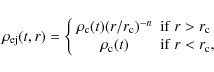
Supernovae observations have confirmed (for the case of SN 1987A, see Arnett 1988)
that at early times, typically a few hours after the supernova
explosion, the matter density of the outer ejecta reaches a power-law
profile as a function of radius given by
![]() .
A kinematical study of the pre-Sedov-Taylor SNR of Kepler (Vink 2008a) confirmed the power-law density profile. The difficulties in attaining a measurement of n makes the comparison of theory with observations difficult. The value of n depends on the properties of the progenitor star and the acceleration of the shock during the explosion. The value n=7, or alternatively an exponential density profile for ejecta (Dwarkadas & Chevalier 1998),
is commonly used to describe type Ia supernovae, which
are believed to result from the explosion of a C/O white
dwarf accreted in a binary system (Hoyle & Fowler 1960). The value n=9
is believed to describe type II supernovae, which result from
the core-collapse of a massive star. If the density of the ambient
medium has a power-law behaviour, namely
.
A kinematical study of the pre-Sedov-Taylor SNR of Kepler (Vink 2008a) confirmed the power-law density profile. The difficulties in attaining a measurement of n makes the comparison of theory with observations difficult. The value of n depends on the properties of the progenitor star and the acceleration of the shock during the explosion. The value n=7, or alternatively an exponential density profile for ejecta (Dwarkadas & Chevalier 1998),
is commonly used to describe type Ia supernovae, which
are believed to result from the explosion of a C/O white
dwarf accreted in a binary system (Hoyle & Fowler 1960). The value n=9
is believed to describe type II supernovae, which result from
the core-collapse of a massive star. If the density of the ambient
medium has a power-law behaviour, namely
![]() ,
self-similar solutions can be found for the density, velocity, and pressure of the interaction region in young SNRs (Chevalier 1982); from dimensional analysis, the time evolution of the radius of the contact discontinuity has the form (Chevalier 1982)
,
self-similar solutions can be found for the density, velocity, and pressure of the interaction region in young SNRs (Chevalier 1982); from dimensional analysis, the time evolution of the radius of the contact discontinuity has the form (Chevalier 1982)
![]() ,
where
,
where
![]() .
.
During the expansion, a colder and denser fluid, the shocked ejecta, slows down in a hotter and less dense fluid, the shocked ISM. Seen in the reference frame of the contact discontinuity, this deceleration is equivalent to a gravity field pushing the shocked ejecta toward the shocked ISM. This instability is at the basis of the familiar RT structures (Chevalier et al. 1992). The structure of the interaction region between the ballistically expanding ejecta and a uniform ISM in young SNR was first explored numerically by Gull (1975,1973), who described how the formation of optical filaments is brought back to the RT instability and provided a qualitative explanation of the amplification of the magnetic field in the interaction region. Given spherical initial conditions, we investigate the growth of RT instabilities in different situations.
In this paper, a steep power-law density ejecta is assumed to expand into a uniform ISM (s=0).
In the innermost part, the common cutoff in radius ![]() is adopted to introduce the density plateau for the ejecta core
is adopted to introduce the density plateau for the ejecta core
where
At a given time ![]() ,
the physical parameters that fix unequivocally the profiles of
,
the physical parameters that fix unequivocally the profiles of ![]() ,
, ![]() ,
and P are the total kinetic energy
,
and P are the total kinetic energy ![]() of the explosion, the total ejecta mass
of the explosion, the total ejecta mass
![]() ,
the circumstellar medium density
,
the circumstellar medium density
![]() and the indices of the power-law density profile of ejecta and ISM, namely (n,s). The outer radius of the inner plateau is given by
and the indices of the power-law density profile of ejecta and ISM, namely (n,s). The outer radius of the inner plateau is given by

|
(2) |
A SNR can be defined to be young when the mass of interstellar matter
The self-similar profiles of mass density ![]() ,
fluid velocity
,
fluid velocity ![]() and pressure P for a young SNR (Chevalier 1983,1982) are used as initial conditions (see Fig. 1).
By assuming spherical symmetry, the self-similar solution is
mapped in a 3D computational grid. At the initial time
t0 = 10 yr, the self-similar profiles are
assumed to be well-established. It is reasonable to assume
that such a spherical symmetry has not yet been significantly modified
by the convective motions grown between the explosion of the supernova
and the time t0. Given the value of t0, we can fix
and pressure P for a young SNR (Chevalier 1983,1982) are used as initial conditions (see Fig. 1).
By assuming spherical symmetry, the self-similar solution is
mapped in a 3D computational grid. At the initial time
t0 = 10 yr, the self-similar profiles are
assumed to be well-established. It is reasonable to assume
that such a spherical symmetry has not yet been significantly modified
by the convective motions grown between the explosion of the supernova
and the time t0. Given the value of t0, we can fix
![]() and therefore the density profile is determined down to r=0, where the origin of the explosion is located. We assume the reasonable values of SNR parameters E0 = 1.6
and therefore the density profile is determined down to r=0, where the origin of the explosion is located. We assume the reasonable values of SNR parameters E0 = 1.6 ![]() 1051 erg and
1051 erg and
![]()
![]()
![]() ,
where
,
where
![]()
![]() 1033 g is the solar mass and the circumstellar medium density
1033 g is the solar mass and the circumstellar medium density
![]() amu
amu ![]() cm-3. The only information concerning the progenitor of the SNR is therefore contained in the index n and the mass
cm-3. The only information concerning the progenitor of the SNR is therefore contained in the index n and the mass
![]() .
For the previous set of parameters, we find the initial radii
of the contact discontinuity, forward shock and reverse shock
to be, respectively,
.
For the previous set of parameters, we find the initial radii
of the contact discontinuity, forward shock and reverse shock
to be, respectively,
![]() pc,
pc,
![]() pc, and
pc, and
![]() pc.
pc.
3 Equation of hydrodynamics in accelerated frame
3.1 Euler equations in laboratory frame
In an inertial cartesian (laboratory) reference frame
![]() ,
the non-relativistic Euler equations of fluid dynamics, in the
absence of viscosity and dissipative processes, are written in the
quasi-conservative form
,
the non-relativistic Euler equations of fluid dynamics, in the
absence of viscosity and dissipative processes, are written in the
quasi-conservative form
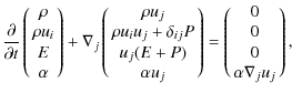
where
Equation (3) is written in conservative form, except the so-called ``quasi-conservative'' form of equation for ![]() .
If the conservative variable
.
If the conservative variable
![]() is used, higher order schemes of shock capturing applied to
multicomponent flows can produce oscillations at the interface of
different fluids (Shyue 1998; Johnsen & Colonius 2006).
is used, higher order schemes of shock capturing applied to
multicomponent flows can produce oscillations at the interface of
different fluids (Shyue 1998; Johnsen & Colonius 2006).
For a shock propagating into an ideal gas, the compression factor at the shock can be expressed as
![]() (Zel'dovich & Raizer 2002), where
(Zel'dovich & Raizer 2002), where ![]() (
(![]() )
is the downstream (upstream) density of the shock and
)
is the downstream (upstream) density of the shock and
![]() is the Mach number in the unshocked medium. In the limit of a very strong shock, as in young SNRs,
is the Mach number in the unshocked medium. In the limit of a very strong shock, as in young SNRs,
![]() and
and
![]() ,
depending only on the thermodynamic properties of the medium.
,
depending only on the thermodynamic properties of the medium.
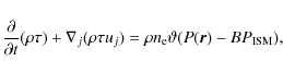
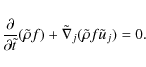
The passive scalar f, representing the mass fraction of ejecta, is initially defined as
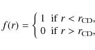
where
The X-ray spectra of SNRs usually exhibit significant emission lines of heavy elements, such as Fe in Kepler (Smith et al. 1989). Therefore, the computation of the X-ray spectrum of SNRs requires an evaluation of the ionization produced by electrons after the passage of the reverse shock. In this paper, we do not compute the ionization state by coupling the hydrodynamics equations with the equations for the evolution of ionization and recombination (for a 1D example of this see Rothenflug et al. 1994). We follow the ionization age, which allows us to compute a posteriori the ionization structure assuming a constant temperature in the fluid element.
An additional passive scalar representing the ionization age, ![]() ,
was introduced into the code, defined as
,
was introduced into the code, defined as
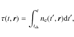
where
where
3.2 Euler equations in comoving reference frame
Now we consider a non-inertial reference frame
![]() .
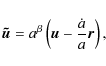
We deal with the simplified case of a purely radially contracting accelerated motion, which was introduced in Martel & Shapiro (1998) as supercomoving coordinate system; the more general case in the presence of rotation is treated in Poludnenko & Khokhlov (2007). The frame
.
We deal with the simplified case of a purely radially contracting accelerated motion, which was introduced in Martel & Shapiro (1998) as supercomoving coordinate system; the more general case in the presence of rotation is treated in Poludnenko & Khokhlov (2007). The frame
![]() is defined by the transformation
is defined by the transformation
![]()
where
where

where we consider the simple case of
From Eqs. (8) and (9), we also have
In 3D, the choice
and
where
Here, for a generic function
![$\displaystyle \left({\frac{\partial g}{\partial t}}\right)_{\vec r} = {1\over a...
...}\right)_{\vec r} - {\tilde H}\vec{r} \cdot(\tilde \nabla g)_{\tilde t}\right],$](/articles/aa/full_html/2010/07/aa12692-09/img109.png)
|
(18) | |
| (19) |
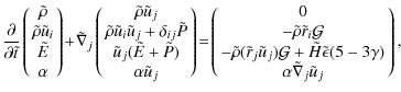
In most physical cases, the bulk motion is accelerated; therefore in the momentum equation written in the non-inertial reference frame a non-inertial force term will appear on the right-hand side. In the right-hand side of Eq. (16), both the second line and the first term of the third line represent the non-inertial force; the second term of the third line, treated as a source term since it acts as the gravitational potential term in the cosmological framework, may create an energy sink, losing the numerical advantage of the conservative form (see Sect. 4 for details).
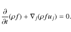
Since it is an advection equation, Eq. (5) is unchanged by the choice of Eq. (15)
Equation (7) changes as follows
In this paper, we consider the early phase of SNR expansion and the transition to the Sedov-Taylor phase, thus the radiative cooling is negligible with respect to the total energy content and the approximation of adiabatic expansion of a perfect fluid is justified. We assume that the fluid mainly consists of fully ionized hydrogen, therefore
The physical time t is related to the time ![]() for
for ![]() and
and ![]() by
by
![\begin{displaymath}%
\tilde t = \frac{t_0}{a_0 ^2} \frac{1}{2\lambda - 1}\left[ 1 - \left(\frac{t_0}{t} \right)^{2\lambda - 1} \right]\cdot
\end{displaymath}](/articles/aa/full_html/2010/07/aa12692-09/img116.png)
In the cases considered,
![\begin{figure}
\par\includegraphics[width=8.5cm,clip]{12692fg1.eps}
\end{figure}](/articles/aa/full_html/2010/07/aa12692-09/img126.png)
|
Figure 1:
Angle-averaged radial density profile at t=50 yr for
|
| Open with DEXTER | |
4 Numerical code
4.1 Set-up
The simulations were performed with the hydrodynamics version of the code RAMSES (Teyssier 2002).
RAMSES was originally developed to study, with the AMR technique,
structure formation in the universe at high spatial resolution. The
solver is based on a second order Godunov scheme. We modified the
constitutive equations of RAMSES as shown in Eqs. (16) and (17) to solve the hydrodynamics flow in an accelerated reference frame expanding according to Eqs. (8)-(10).
The modifications concern the hydrodynamic solver routines and the
external gravity routine, because the change of reference frame
introduces a non-inertial force in the Euler equations, which can be
treated as a source term in the momentum and energy equation. We also
introduced an additional variable ![]() ,
treated as a passive scalar in Eqs. (3) and (16), to change locally the equation of state and two more passive scalars (see Sect. 3.1 for details).
,
treated as a passive scalar in Eqs. (3) and (16), to change locally the equation of state and two more passive scalars (see Sect. 3.1 for details).
The simulations were performed over three levels of refinement, of value l=7-9, corresponding to a cartesian grid with a number of cells 1283, 2563, and 5123,
respectively. The effective maximal resolution attained in the
interaction region at the set-up of the simulation is 0.4/512
![]()
![]() 10-4
10-4 ![]() .
Our 3D numerical simulations were carried out across one octant of a sphere.
.
Our 3D numerical simulations were carried out across one octant of a sphere.
The refinement algorithm is applied to the surfaces of the
contact discontinuity and the two shocks. The surface of the contact
discontinuity is detected by means of the gradient in the tracing
function f (see Sect. 3.1),
rather than the density gradient; in this way, the effectiveness
of the detection is independent of the parameters (n,s).
The forward and reverse shocks are detected by measuring the pressure
discontinuity. The advantage is that the pressure discontinuity is
greater than the discontinuities in density or radial velocity and
independent of the assumptions about the density power-law index in the
free expansion medium and the equation of state of the gas in the
interaction region. Figure 1 shows the angle-averaged radial density profile at t=50 yr for
![]() ,
or
(n,s) = (7,0), and
,
or
(n,s) = (7,0), and
![]() with 1-3 levels of refinement. The resolution of the
RT structures is crucially improved by applying the AMR.
with 1-3 levels of refinement. The resolution of the
RT structures is crucially improved by applying the AMR.
During the expansion of a young SNR, the only dynamically interesting region, represented by the interaction region, occupies a fraction of about 40% (and constant during the self-similar regime) of the whole remnant volume. Moreover the Kelvin-Helmoltz instabilities triggered by the growth of the RT finger-like structures during the ``self-similar'' phase lead to a strongly turbulent phase. Therefore, AMR hydrodynamic simulation that attempts to spatially resolve the growth of the RT instabilities must refine over an increasingly large relative volume. The contact discontinuity turns out to be the most computationally expensive region of the flow. In contrast, the core region within the power-law ejecta, where the value of the uniform density is fixed by mass conservation, can be easily handled at the lowest possible refinement level. In this context, the AMR technique, combined with the approach of Moving Computational Grid, is found to be suitable.
We define the boundary conditions of the conservative variables
in the corresponding six ghost zones. Since we treat 1/8 of the
volume of the remnant sphere, in some ghost zones (three) the
boundary condition is inflow, produced by the advection of the
interstellar material, and in some other ghost zones (three) the
boundary condition is reflexive, according to the location of the
interface of the ghost cell. Changes in the order of the assignment of
the ghost cells significantly change neither the resulting intercell
flow at the shock nor the physical content of the result. In the
laboratory rest frame, the ISM is cold and stationary:
![]() .
In the shock frame, this implies that the ISM is advected onto the SNR shock surface with a velocity field given by
.
In the shock frame, this implies that the ISM is advected onto the SNR shock surface with a velocity field given by
![]() (see Eq. (11)).
Therefore, a linear interpolation (second order) for the
reconstruction of the velocity field at the boundaries more clearly
describes the inflowing material.
(see Eq. (11)).
Therefore, a linear interpolation (second order) for the
reconstruction of the velocity field at the boundaries more clearly
describes the inflowing material.
The time step is controlled using a standard Courant factor
stability constraint. Based on our expanding coordinate system, we also
included a time step limitation, where a(t) is not allowed to vary by more than ![]() over the time step.
over the time step.
The cartesian coordinate system that we use here is not well-adapted to spherically symmetric objects such as SNRs and spurious geometrical effects are expected. It has long been known that an Eulerian code should take care of its violation of Galileian invariance: a turbulent phenomenon observed in a fixed computational grid can disappear if it is observed from a computational grid moving at constant velocity with respect to the fixed grid. The goal of our comoving coordinate system is precisely to eliminate this effect. This improvement does, however, have the problem, which is common to all shock capturing schemes dealing with stationary shocks, of the so-called ``odd-even decoupling'' and the associated carbuncle phenomenon (Peery & Imlay 1988; Quirk 1994; Pandolfi & D'Ambrosio 2001), namely a disturbance in the computation of the flow emerging when the shock direction is aligned with one of the grid coordinate directions. This effect may be amplified when a flow converges in a cell from different directions, as in the case of spherical flow on a cartesian mesh. The result can strongly deform the shock surface and form ripples or bubble-like regions of local sub-density. Local changes to the solver were proposed (Kifonidis et al. 2003), based on an algorithm for the detection of the shock. Reconstruction of the interface values of the state variables is performed, but in the cells detected by that algorithm a more diffusive solver is used, such as HLL, HLLC or Lax-Friedrichs (Toro 1999), while in all the remaining regions a conventional Riemann exact solver or an approximate Roe solver can be used. Solving this long-standing issue is beyond the scope of this paper, so we did not implement these possible fixes here.
4.2 Integration method
We briefly recall the main steps of the integration method of RAMSES (Toro 1999).
In the absence of a gravitational potential,
the three-dimensional hydrodynamic Euler equations can be written
in the conservative form as (see Eq. (3))
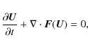
where
|
(24) |
Apart from a smooth flow of the conservative variables
|
(25) |
|
(26) |
|
(27) |
The conservative system can then be written
|
||
|
(28) |
This integral form remains exact for the corresponding Euler system since no approximation has been made. Since the intercell flux is computed at time
In presence of a source term, Eq. (23) becomes
where
The time centered fluxes
where
Although the integration of the source term Sn+1/2i,j,k in Eq. (30) is of second order in time, higher order methods, such as Rosenbrock (Kaps & Rentrop 1979), can be chosen.
5 Application to SNR
5.1 Growth of Rayleigh-Taylor structures
![\begin{figure}
\par\includegraphics[width=16.5cm,clip]{12692fg2.eps}
\end{figure}](/articles/aa/full_html/2010/07/aa12692-09/img168.png)
|
Figure 2:
Angle-averaged radial density profile at various ages for
|
| Open with DEXTER | |
![\begin{figure}
\par\includegraphics[width=8.8cm,clip]{12692fg3.eps}
\end{figure}](/articles/aa/full_html/2010/07/aa12692-09/img169.png)
|
Figure 3:
Temporal evolution of the forward shock and reverse shock radii for
|
| Open with DEXTER | |
Many developed codes have satisfactorily tackled the growth of RT instabilities as a mandatory validity test. In contrast to previous treatments, we consider the evolution of a full octant of the SNR. Thus, within a larger SNR volume, a large number of RT-instabilitiy lengthscales, spread over a wider range, sum together. In other words, the growth of RT instabilities is more accurately described not only with high spatial resolution, but also with volumes comparable to the global SNR volume. In particular, since the initial departures from the spherical symmetry are sampled over a larger surface, the initial phase of the RT growth is statistically more accurately described (see Sect. 6.3).
Even in the case of a stationary advective shock, a small volume has been dealt with, in the SNR literature, in comparison with the volume of the interaction region. The description here provides a more comprehensive overview of the dynamics of RT instabilities in the SNR.
The simulations presented here cover three phases of the adiabatic SNR expansion (see Fig. 2): the self-similar expansion (Chevalier 1982) with an exponent ![]() depending on the properties of the ejecta and the ISM, i.e. on (n,s); the second phase, not self-similar, representing the transition to the Sedov-Taylor regime (
depending on the properties of the ejecta and the ISM, i.e. on (n,s); the second phase, not self-similar, representing the transition to the Sedov-Taylor regime (
![]() ); and the third phase (Sedov-Taylor), with a blast wave radius
); and the third phase (Sedov-Taylor), with a blast wave radius ![]() that expands as
that expands as
![]() ,
for s=0, and
,
for s=0, and
![]() .
The transition between the two self-similar phases is shown by means of
various snapshots of the angle-averaged density in Fig. 2. In this case, we assume that
.
The transition between the two self-similar phases is shown by means of
various snapshots of the angle-averaged density in Fig. 2. In this case, we assume that
![]() ,
or
(n,s) = (7,0), and
,
or
(n,s) = (7,0), and
![]() in the whole simulation box. The inward motion of the reverse shock and
the progressive establishment of the Sedov-Taylor profile is manifest.
We extended our computation until values of time t when the inward motion of
in the whole simulation box. The inward motion of the reverse shock and
the progressive establishment of the Sedov-Taylor profile is manifest.
We extended our computation until values of time t when the inward motion of
![]() has reached the inner core, and show that during the transition to the
Sedov-Taylor phase, the angle-averaged profile is not significantly
altered by the development of the RT instability. The 1D
Sedov-Taylor density profile is superimposed in the last three panels
of Fig. 2, by assuming that the Sedov-Taylor phase is fully established at t = 5
has reached the inner core, and show that during the transition to the
Sedov-Taylor phase, the angle-averaged profile is not significantly
altered by the development of the RT instability. The 1D
Sedov-Taylor density profile is superimposed in the last three panels
of Fig. 2, by assuming that the Sedov-Taylor phase is fully established at t = 5 ![]()
![]() ,
where
,
where
![]()
![]()
![]() (Truelove & McKee 1999). Compared with the original version of the code in the case of a spherical Sedov blast wave (Teyssier 2002),
we note the improvement in the resolution of the compression factor; in
that previous work relatively small values of final output times had
been considered, the aim being to test the code.
(Truelove & McKee 1999). Compared with the original version of the code in the case of a spherical Sedov blast wave (Teyssier 2002),
we note the improvement in the resolution of the compression factor; in
that previous work relatively small values of final output times had
been considered, the aim being to test the code.
In Fig. 3, the
outermost value of the position of the forward shock and the innermost
value of the position of the reverse shock in 3D are compared with
the semi-analytical 1D solution of Truelove & McKee (1999). The units used here correspond to
![]() (pc) =
(pc) =
![]() and
and
![]() (yr) =
(yr) =
![]() ,
where
,
where
![]()
![]()
![]() is the mean mass per hydrogen nucleus assuming cosmic abundances.
In particular, the inward motion of the reverse shock is
compared with the solution of Truelove & McKee (1999); in the case
(n, s) = (7, 0), we find agreement within
is the mean mass per hydrogen nucleus assuming cosmic abundances.
In particular, the inward motion of the reverse shock is
compared with the solution of Truelove & McKee (1999); in the case
(n, s) = (7, 0), we find agreement within ![]() between our 3D simulation and the 1D solution of Truelove & McKee (1999).
The radius of the reverse shock is strongly modified by the
RT instability where the innermost value is chosen.
In contrast, the radius of the forward shock is unequivocally
defined, since it is not perturbed by the RT instabilities for the
physically relevant values of (n,s) (see also Fig. 5).
between our 3D simulation and the 1D solution of Truelove & McKee (1999).
The radius of the reverse shock is strongly modified by the
RT instability where the innermost value is chosen.
In contrast, the radius of the forward shock is unequivocally
defined, since it is not perturbed by the RT instabilities for the
physically relevant values of (n,s) (see also Fig. 5).
In Fig. 4 (upper panel), the mass fraction
![]() ,
defined in Eq. (4), is shown in a planar slice parallel to the coordinate plane XY at time t=100 yr (left) and t=500 yr (right); in this case,
,
defined in Eq. (4), is shown in a planar slice parallel to the coordinate plane XY at time t=100 yr (left) and t=500 yr (right); in this case,
![]() ,
or
(n,s) = (7,0) and
,
or
(n,s) = (7,0) and
![]() .
The mixture of the two media, shocked ejecta and shocked ISM,
as well as the deformation of the contact discontinuity surface
appear at intermediate values of
.
The mixture of the two media, shocked ejecta and shocked ISM,
as well as the deformation of the contact discontinuity surface
appear at intermediate values of
![]() .
In the middle panel, the matter density is shown with the same
spatial extension and times as in the upper panel. In the lower
panel, an estimate of the frequency emissivity
.
In the middle panel, the matter density is shown with the same
spatial extension and times as in the upper panel. In the lower
panel, an estimate of the frequency emissivity ![]() produced by bremsstrahlung in purely hydrogen gas is shown, integrated
along the line of sight towards the reader. Only the interaction region
where the temperature is high contributes to the emissivity. The
emissivity
produced by bremsstrahlung in purely hydrogen gas is shown, integrated
along the line of sight towards the reader. Only the interaction region
where the temperature is high contributes to the emissivity. The
emissivity ![]() is computed based on the assumption that the plasma is optically thin (bremsstrahlung). Therefore, the emissivity is given by
is computed based on the assumption that the plasma is optically thin (bremsstrahlung). Therefore, the emissivity is given by
![]()
![]()
![]() ,
where
,
where ![]() is the electron number density and
is the electron number density and ![]() is the electron temperature given by the perfect gas equation of state such that
is the electron temperature given by the perfect gas equation of state such that
![]() ,
where
,
where ![]() is the mean molecular weight,
is the mean molecular weight,
![]()
![]() 10-24 g is the proton mass, and
10-24 g is the proton mass, and
![]()
![]() 10-16 erg/K is the Boltzmann constant. For simplicity, in this case we chose
10-16 erg/K is the Boltzmann constant. For simplicity, in this case we chose ![]() ,
corresponding to the case of fully ionized hydrogen. We implicitly assumed that
,
corresponding to the case of fully ionized hydrogen. We implicitly assumed that
![]() ,
where
,
where ![]() is the ion temperature, while at an early stage the SNR is not yet
completely thermalized. A more detailed study should account for
inclusion of the evolution of
is the ion temperature, while at an early stage the SNR is not yet
completely thermalized. A more detailed study should account for
inclusion of the evolution of
![]() ,
but this indicative diagram provides nevertheless a starting point.
,
but this indicative diagram provides nevertheless a starting point.
In Fig. 5, a 3D large view image of the density field in the full simulation box is shown. This picture shows that while the sphericity of the forward shock surface is maintained since the RT instabilities do not reach the shock, the reverse shock surface is strongly modified. The large relative volume of the refinement region can be clearly seen.
In Fig. 6, the streamlines of the velocity field in the reference frame of the contact discontinuity in distinct snapshots show the development of the chaotic flow in the interaction region due to the convective motions. As the time proceeds, the central density decreases and the relative size of the region of turbulence increases.
![\begin{figure}
\par\includegraphics[width=7.5cm,clip]{12692fg4a.eps}\includegrap...
...ip]{12692fg4e.eps}\includegraphics[width=7.5cm,clip]{12692fg4f.eps}
\end{figure}](/articles/aa/full_html/2010/07/aa12692-09/img193.png)
|
Figure 4:
Snapshots at two distinct ages (t=100 yr at left; t=500 yr at right) for
|
| Open with DEXTER | |
For a general acceleration field g, the initial growth of
small amplitude perturbations at the accelerated contact discontinuity
between two incompressible fluids is exponential with a growth
rate ![]() .
The quantity
.
The quantity ![]() is related to the wavenumber k by the relation
is related to the wavenumber k by the relation
![]() ,
where
,
where
![]() and
and ![]() ,
, ![]() are the densities of the two adjacent media at the contact
discontinuity. At later times, the growth of the ripples at the
contact discontinuity enters the so-called ``self-similar phase''; this
phase was first quantitatively analyzed by Fermi & von Neumann (1953). The self-similar growth of the RT instable structures is governed by the equation
are the densities of the two adjacent media at the contact
discontinuity. At later times, the growth of the ripples at the
contact discontinuity enters the so-called ``self-similar phase''; this
phase was first quantitatively analyzed by Fermi & von Neumann (1953). The self-similar growth of the RT instable structures is governed by the equation
where the constant
![\begin{displaymath}%
\frac{H(t)}{r_{\rm CD}(t_0)} = \frac{4\delta A (\lambda-1)}...
...bda}\left[\left(\frac{t}{t_0}\right)^{\lambda/2} - 1\right]^2,
\end{displaymath}](/articles/aa/full_html/2010/07/aa12692-09/img202.png)
where
![\begin{figure}
\par\includegraphics[width=8.5cm,clip]{12692fg5.eps}
\end{figure}](/articles/aa/full_html/2010/07/aa12692-09/img204.png)
|
Figure 5:
The three-dimensional density in the full simulation box of side L = 4.2 pc is shown at t=500 yr for
|
| Open with DEXTER | |
![\begin{figure}
\par\includegraphics[width=8cm,clip]{12692fg6a.eps}\includegraphi...
...clip]{12692fg6c.eps}\includegraphics[width=8cm,clip]{12692fg6d.eps}
\end{figure}](/articles/aa/full_html/2010/07/aa12692-09/img205.png)
|
Figure 6:
Snapshots showing streamlines of velocity field superposed to matter density for
|
| Open with DEXTER | |
The limited spatial resolution attainable at the contact discontinuity with a cartesian grid makes it hard to verify early time exponential growth (Fermi & von Neumann 1953), prior to the self-similar regime.
5.2 Non-thermal particles in the shocked ISM
Multiwavelength surveys have inferred that cosmic-ray acceleration can be efficient in young SNRs (see Vink 2008b, and references therein). The idea at the basis of particle acceleration at SNR shocks is the Fermi first-order mechanism of acceleration, namely that particles accelerate by repeatedly crossing the shock and colliding at every passage with magnetic turbulences. Therefore, beside other parameters, the efficiency of acceleration depends on the intensity and the spatial configuration of the magnetic field. The X-ray detections of narrow synchrotron emitting filaments at SNR shocks indicate magnetic field intensities up to 1 mGauss (Vink & Laming 2003; Lazendic et al. 2003; Bamba et al. 2003). Magnetic field amplification at shocks has been interpreted as the result of turbulence in the postshock material (Giacalone & Jokipii 2007) or cosmic-ray induced streaming instability (Bell 2004; Amato & Blasi 2009).
The SNR hydrodynamics can be modified by efficient particle acceleration at the forward shock (Decourchelle et al. 2000). Therefore, a complete numerical description of the SNR expansion should take into account the feedback of the non-thermal population of particles on the dynamics of the SNR, i.e., the system of Euler equations (Eqs. (3)) should be coupled to the equation for the cosmic-ray phase-space distribution function.
Blondin & Ellison (2001) investigated this scenario by changing the adiabatic index ![]() globally. They found that the development of the RT instability
was relatively unaffected and the main effect was that, because the
compression ratio increases and the shocked region shrinks when
globally. They found that the development of the RT instability
was relatively unaffected and the main effect was that, because the
compression ratio increases and the shocked region shrinks when ![]() decreases, the RT fingers approached the forward shock and could even reach it for
decreases, the RT fingers approached the forward shock and could even reach it for
![]() .
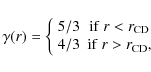
We adopt a similar approach but investigate when particle acceleration
is efficient at the forward shock only. We call this the hybrid case in
the remainder of the paper. A local equation of state of the form
.
We adopt a similar approach but investigate when particle acceleration
is efficient at the forward shock only. We call this the hybrid case in
the remainder of the paper. A local equation of state of the form
![]() is assumed. The shocked ISM is initialized as a relativistic gas
(dominated by cosmic rays) and the shocked ejecta is initialized
as a non-relativistic gas such that
is assumed. The shocked ISM is initialized as a relativistic gas
(dominated by cosmic rays) and the shocked ejecta is initialized
as a non-relativistic gas such that
the corresponding
The initial adiabatic ![]() distribution in Eq. (34) should provide a more realistic representation of forward shock accelerating particles than a
distribution in Eq. (34) should provide a more realistic representation of forward shock accelerating particles than a
![]() uniform
distribution across the whole interaction region. There has been
relatively little observational or theoretical evidence that particle
acceleration is very efficient at the reverse shock (Ellison et al. 2005). An interesting result of that simulation is that the density behind the reverse shock is lower
than behind the forward shock in the self-similar solution, at least for n = 7 (Fig. 8 as opposed to Fig. 1). This may hinder the development of the RT fingers.
uniform
distribution across the whole interaction region. There has been
relatively little observational or theoretical evidence that particle
acceleration is very efficient at the reverse shock (Ellison et al. 2005). An interesting result of that simulation is that the density behind the reverse shock is lower
than behind the forward shock in the self-similar solution, at least for n = 7 (Fig. 8 as opposed to Fig. 1). This may hinder the development of the RT fingers.
6 Discussion
6.1 Intrinsic issues in the stationary advective shock problem
In simulating stationary advective shocks, numerical instabilities related to the ``carbuncle phenomenon'' can be found by using the Roe solver. The carbuncle phenomenon was first observed by Peery & Imlay (1988) in blunt body simulations using Roe's method and numerically studied in detail by Quirk (1994), and has remained a crucial numerical issue (Pandolfi & D'Ambrosio 2001; Xu & Li 2001) until recently (Nishikawa & Kitamura 2008). The carbuncle phenomenon is considered to be a spurious numerical effect affecting hydrodynamic simulations when the intercell flow is aligned with one of the coordinate directions of the computational grid; it shows up when a supersonic shock, or more generally a discontinuity in the flow variables, is comoving with the computational grid. The Riemann solver produces unphysical ripples of the shock and in the post-shock region, which at late times can modify the structure of the shock surface itself. The numerical methods that are likely to produce carbuncle phenomenon have not yet been unequivocally identified, an attempt to classify them being Dumbser et al. (2003).
The so-called ``H-correction'' (Stone et al. 2008), which consists of introducing an anisotropic dissipative flux in the direction perpendicular to the direction of propagation of the shock, cannot be applied here. We did not add a diffusive term in the intercell flux, which is usually adopted to avoid the growth of numerical instabilities. The addition of artificial viscosity could damp physical effects emerging during the development of the RT instabilities, which we are interested in studying in detail. For the same reason, we did not use more diffusive solvers such as HLL or HLLC or Lax-Friedrichs (Toro 1999).
In the case of supernova core-collapse simulations, a possible solution has been to compute the intercell flux in the zones of strong shock with an Einfeldt solver (Quirk 1994,1997), while all the other grids in the computational box are treated with a less diffusive Riemann solver (Kifonidis et al. 2003). We preferred not to introduce a solver-switching algorithm to avoid introducing other spurious effects possibly arising from the matching of the intercell fluxes.
To avoid the numerical instability occurring at the stationary shock, we used the exact solver. The failure of the Roe solver manifests itself in local fluctuations of density in regions behind the shock and strong deformations of the shock surface, which grow as the non-linear regime of RT instabilities is reached; consequent unphysical effects due to velocity shear, resembling Kelvin-Helmholtz instabilities, develop at the same time. Both effects are absent if the shock is not stationary with respect to the computational grid and depend on the chosen simulation parameters, for instance CFL number or interpolation scheme of conservative variables; thus they must be attributed to the choice of the solver. The choice of the exact solver did not significantly increase the computational time.
6.2 Quasi-comoving grid
A different solution to the carbuncle problem could involve defining a computational grid that drifts with respect to the SNR, slowly enough to follow the expansion of the remnant for a long time and to avoid boundary reflections possibly occurring with a remnant overtaking the grid. However, this is an even less viable solution since, as shown in the following, the angle-averaged density profiles strongly deviate from the expected compression ratio at the two shocks. In contrast, as shown earlier, in the case of an exactly comoving computational grid, the post-shock ripples average to zero.
![\begin{figure}
\par\includegraphics[width=8.8cm,clip]{12692fg7.eps}
\vspace*{2mm}
\end{figure}](/articles/aa/full_html/2010/07/aa12692-09/img209.png)
|
Figure 7: The protruding RT
structures measured in our simulations at different times are quite
well reproduced by the exact solution H(t) with
|
| Open with DEXTER | |
![\begin{figure}
\par\includegraphics[width=8.8cm,clip]{12692fg8.eps}
\vspace*{2mm}
\end{figure}](/articles/aa/full_html/2010/07/aa12692-09/img210.png)
|
Figure 8:
Angle-averaged radial density profile shown at distinct ages for
|
| Open with DEXTER | |
Independently of the initial density profile, i.e., of the value of ![]() ,
the self-similar regime slows down towards the Sedov-Taylor solution, which has a self-similar exponent equal to
,
the self-similar regime slows down towards the Sedov-Taylor solution, which has a self-similar exponent equal to
![]() .
Therefore, the contact discontinuity in the computational grid will
progressively acquire a drift velocity depending on the physical
parameters of the remnant. To test the numerical stability of the
shock, we introduced a ``quasi-comoving'' grid, whose small drift with
respect to the contact discontinuity velocity is parametrized by
.
Therefore, the contact discontinuity in the computational grid will
progressively acquire a drift velocity depending on the physical
parameters of the remnant. To test the numerical stability of the
shock, we introduced a ``quasi-comoving'' grid, whose small drift with
respect to the contact discontinuity velocity is parametrized by
![]() :
:
![]() .
.
![\begin{figure}
\par\includegraphics[width=8.9cm,clip]{12692fg9a.eps}\hspace*{4mm}
\includegraphics[width=8.75cm,clip]{12692fg9b.eps}
\end{figure}](/articles/aa/full_html/2010/07/aa12692-09/img214.png)
|
Figure 9:
Matter density in a comoving planar slice parallel to the coordinate plane XY at height z=0.1 |
| Open with DEXTER | |
The quasi-comoving grid, even with the Roe solver, smears out the
ripples produced behind the forward shock surface by the stationarity
of the computational grid, therefore locally is odd-even
instability-free (see Fig. 9).
However, the angle-averaged density profile, even at the first
time-steps, is affected by an error in the compression factor at the
two shocks (see Fig. 10,
upper panel), the position of the shock being unchanged. The
redistribution of the mass through the two shocks in the presence of a
grid drift (over-compression at reverse shock and under-compression at
forward shock) is to be attributed to the mapping of a spherically
symmetric object on a cartesian grid. It manifests itself during
the transition to the Sedov-Taylor phase in terms of an error of ![]() in the resolution of the compression at the shock, and should be
considered an intrinsic limit of the approach used here. This error
does not depend on the number of levels of the AMR (see Fig. 10,
lower panel). As a consequence, even if a larger number of
computational cells is considered, the angle-averaged value at the
shock does not fulfill the value of the compression predicted by the
Rankine-Hugoniot conditions. In contrast, for an exactly
comoving grid, even with the Roe solver, strong deformations of
the shock surface are triggered by the numerical instability but the
compression at the shocks is preserved. The same difference of results
between the exactly comoving and quasi-comoving has been found with
the exact Riemann solver, shown in Fig. 10.
in the resolution of the compression at the shock, and should be
considered an intrinsic limit of the approach used here. This error
does not depend on the number of levels of the AMR (see Fig. 10,
lower panel). As a consequence, even if a larger number of
computational cells is considered, the angle-averaged value at the
shock does not fulfill the value of the compression predicted by the
Rankine-Hugoniot conditions. In contrast, for an exactly
comoving grid, even with the Roe solver, strong deformations of
the shock surface are triggered by the numerical instability but the
compression at the shocks is preserved. The same difference of results
between the exactly comoving and quasi-comoving has been found with
the exact Riemann solver, shown in Fig. 10.
As a consequence, during the transition to the Sedov-Taylor solution,
the generation of a numerical error must be expected in the compression
at the shock. A possible solution is the introduction of a grid
velocity given by
![]() .
.
6.3 Cosmic-ray-dominated blast wave
![\begin{figure}
\par\includegraphics[width=8.8cm,clip]{12692fg10.eps}\vspace*{1.5mm}
\end{figure}](/articles/aa/full_html/2010/07/aa12692-09/img217.png)
|
Figure 10:
Angle-averaged radial density profiles between the reverse shock and the forward shock at time t=12 yr = 0.0063
|
| Open with DEXTER | |
![\begin{figure}
\par\includegraphics[width=8.8cm,clip]{12692fg11.eps}
\end{figure}](/articles/aa/full_html/2010/07/aa12692-09/img218.png)
|
Figure 11:
Angle-averaged radial profile of the mass fraction of the ejecta f shown at distinct ages for
|
| Open with DEXTER | |
![\begin{figure}
\par\includegraphics[width=8.8cm,clip]{12692fg12.eps}
\end{figure}](/articles/aa/full_html/2010/07/aa12692-09/img219.png)
|
Figure 12:
The protrusion of RT structures measured in our simulations in units of
the corresponding self-similar position of the contact discontinuity,
whose surface is directly modified by the instabilities; the uniform
|
| Open with DEXTER | |
For s = 0, a convenient case to consider when analyzing the growth of RT structures is n
= 7, for which the width of the interaction region is large, thus the
elongation of the instabilities can be studied for a longer time and
the forward shock remains unaffected. The effect of changing the
equation of state on the growth of the instabilities is represented in
Fig. 11. It shows how far
the RT fingers reach during their growth (100 yr) and when
they are fully developed (500 yr). At 500 yr,
the fraction of ejecta material transported well into the shocked
ISM
(at
![]() ,
say) is lower in the hybrid case. Nevertheless, the outermost ejecta
reach nearly as far, and very close to the forward shock.
,
say) is lower in the hybrid case. Nevertheless, the outermost ejecta
reach nearly as far, and very close to the forward shock.
In the hybrid case, the position of the reverse shock is
unaffected by a relativistic gas at the forward shock, and the
departure from the self-similar position is less than ![]() .
If the relativistic gas is uniformly distributed across the whole
interaction region, the departure of the reverse shock from the
self-similar position is of the order of
.
If the relativistic gas is uniformly distributed across the whole
interaction region, the departure of the reverse shock from the
self-similar position is of the order of ![]() .
Similar deviations have been found by Blondin & Ellison (2001), who considered however a relatively small angular region in the cases
(n,s) = (7,2) or
(n,s) = (12,0). The bumps in f(r) found at
.
Similar deviations have been found by Blondin & Ellison (2001), who considered however a relatively small angular region in the cases
(n,s) = (7,2) or
(n,s) = (12,0). The bumps in f(r) found at
![]() originate in the RT structures themselves, independent of the
originate in the RT structures themselves, independent of the ![]() distribution. In the two cases
distribution. In the two cases
![]() and
and
![]() ,
the width of the shocked ISM region (
,
the width of the shocked ISM region (
![]() )
shrinks from 0.18 to 0.10. Comparable shrinking has been
found in the angle-average analysis of X-ray observations of
Tycho's SNR (Warren et al. 2005).
)
shrinks from 0.18 to 0.10. Comparable shrinking has been
found in the angle-average analysis of X-ray observations of
Tycho's SNR (Warren et al. 2005).
As shown in Fig. 12,
the elongation of the RT structures in the hybrid case decelerates
relative to the non-relativistic case. The deceleration is caused by
the higher density gradient ahead of the contact discontinuity
(cf. Figs. 8 and 1). This can be easily understood because the RT growth rate ![]() depends through A on the average ratio of the two densities in the interaction region, i.e.,
depends through A on the average ratio of the two densities in the interaction region, i.e.,
![]() (cf. Fig. 8), thus lower density ratios produce lower growth rates (see Fig. 12). The higher compression in the ISM shocked region in the hybrid case produces the slowing down shown in Figs. 11 and 12. When
(cf. Fig. 8), thus lower density ratios produce lower growth rates (see Fig. 12). The higher compression in the ISM shocked region in the hybrid case produces the slowing down shown in Figs. 11 and 12. When
![]() on both sides as in Blondin & Ellison (2001),
on both sides as in Blondin & Ellison (2001),
![]() remains larger than 1
and the RT fingers reach further than in the hybrid case at
remains larger than 1
and the RT fingers reach further than in the hybrid case at
![]() .
.
The region which drives the instability at very early time is that part
of the density profile where density decreases outwards
(see Fig. 1). This is entirely on the ejecta side and therefore unaffected by changing ![]() in the shocked ISM (see Fig. 11).
In other words, at a very early stage, when the instabilities grow
exponentially, the process occurs locally in the outer ejecta and
the cosmic rays cannot affect it. However, particle acceleration
will be able to affect RT structures as soon as they reach the
shocked ISM, since the density gradient of the shocked ISM is higher
for higher compression ratios. For the reasons explained above, a
phenomenological equation of the type of Eq. (32)
can only qualitatively reproduce the global behaviour. We could not
find a more accurate description in this case. A comparison of
Figs. 12 with 7 of Blondin & Ellison (2001)
might indicate that the large fluctuations they observed in the
late-time radial extent of RT structures are not an intrinsic
property of the instability but a result of the too small physical size
of the region considered.
in the shocked ISM (see Fig. 11).
In other words, at a very early stage, when the instabilities grow
exponentially, the process occurs locally in the outer ejecta and
the cosmic rays cannot affect it. However, particle acceleration
will be able to affect RT structures as soon as they reach the
shocked ISM, since the density gradient of the shocked ISM is higher
for higher compression ratios. For the reasons explained above, a
phenomenological equation of the type of Eq. (32)
can only qualitatively reproduce the global behaviour. We could not
find a more accurate description in this case. A comparison of
Figs. 12 with 7 of Blondin & Ellison (2001)
might indicate that the large fluctuations they observed in the
late-time radial extent of RT structures are not an intrinsic
property of the instability but a result of the too small physical size
of the region considered.
7 Conclusions
We have adapted the AMR code RAMSES, which is based on a second order Godunov method in an expanding frame called ``supercomoving coordinates'', to follow the evolution of SNRs. In this approach, not only the space-time variables have been modified but also the hydrodynamics variables. The comoving coordinate system allows an eighth of the total volume of the SNR to be described, which is much larger than previously considered. A longer time interval can be investigated, of the order of thousands of years, until the transition to the asymptotic Sedov-Taylor phase. Such a large volume allows the convective instabilities to be modeled more accurately since it considers not only the shortest wavelengths, which have the greatest growth rate, but also the longer wavelengths, which grow more slowly but make a significant contribution to the morphology of the SNR over time-scales of thousands of years. Our larger spatial sampling allows a statistically more accurate description of the instabilities.
The great advantage of the method adopted here is that it minimizes the velocity of the fluid relative to the grid, and the numerical diffusion at the contact discontinuity, where the instability should develop. In the comoving reference frame, the contact discontinuity, in the absence of distortions due to convective instabilities and before the transition to the Sedov-Taylor phase, would be exactly stationary in time. The analytical non-inertial term resulting from this coordinate transformation is strictly equivalent to a gravitational acceleration: the Euler equations have therefore been integrated with the corresponding additional source terms.
The elongation of the Rayleigh-Taylor structures slowly reaches the asymptotic behaviour ![]() ,
by direct solution of the self-similar theory according to the
assumption of a self-similar acceleration instead of a constant
acceleration.
,
by direct solution of the self-similar theory according to the
assumption of a self-similar acceleration instead of a constant
acceleration.
We have presented a simple way to numerically investigate the effect of efficient particle acceleration at the forward shock, approximating the shocked ISM as a relativistic gas and the shocked ejecta as a non-relativistic gas, with a different adiabatic exponent in each fluid. The density behind the forward shock may be higher than at the reverse shock in that case. A deceleration in the protruding of RT structures is caused by the higher compression of the shocked ISM. The conclusion of Blondin & Ellison (2001) that the RT fingers can travel very close to the shock in the presence of accelerated particles remains valid. The elongation of the instabilities has here been more precisely quantified. We propose that this will allow us to understand why ejecta are found very close to the blast wave in the remnant of SN 1006 (Cassam-Chenaï et al. 2008). The set-up of the code presented here will allow future studies of the back-reaction of particle acceleration on the SNR evolution.
AcknowledgementsThe numerical simulations have been performed with the DAPHPC cluster at CEA, DSM, for which the technical assistance is gratefully acknowledged. F.F. wishes to thank for useful discussions K. Kifonidis, E. Muller, A. Poludnenko. The work of F.F. was supported by CNES (the French Space Agency) and was carried out at Service d'Astrophysique, CEA/Saclay and partially at the Center for Particle Astrophysics and Cosmology (APC) in Paris. The authors are also grateful to the anonymous referee for the useful suggestions.
References
- Amato, E, & Blasi, P. 2009, MNRAS, 392, 1591 [NASA ADS] [CrossRef] [Google Scholar]
- Arnett, W. D. 1988, ApJ, 331, 377 [NASA ADS] [CrossRef] [Google Scholar]
- Bamba, A., Yamazaki, R., Yoshida, T., et al. 2005, ApJ, 621, 793 [NASA ADS] [CrossRef] [Google Scholar]
- Bell, A. R. 2004, MNRAS, 353, 550 [Google Scholar]
- Bietenholz, M. F., Bartel, N., & Rupen, M. P. 2001, ApJ, 557, 770 [NASA ADS] [CrossRef] [Google Scholar]
- Blondin, J. M., & Ellison, D. C. 2001 ApJ, 560, 244 [Google Scholar]
- Cassam-Chenaï, G. Hughes, J. P., Reynoso, E. M., et al. 2008, ApJ, 680, 1180 [NASA ADS] [CrossRef] [Google Scholar]
- Chevalier, R. A. 1982, ApJ, 258, 790 [Google Scholar]
- Chevalier, R. A. 1983, ApJ, 272, 765 [NASA ADS] [CrossRef] [Google Scholar]
- Chevalier, R. A., Blondin, J. M., & Emmering, R. T. 1992, ApJ, 392, 118 [NASA ADS] [CrossRef] [Google Scholar]
- Decourchelle, A., Ellison, D., & Ballet, J. 2000, A&A, 543, L57 [Google Scholar]
- Dumbser, M., Moschetta, J.-M., & Gressier, J. 2004, J. Comput. Phys., 197, 647 [NASA ADS] [CrossRef] [Google Scholar]
- Dwarkadas, V. V. 2000, ApJ, 541, 418 [NASA ADS] [CrossRef] [Google Scholar]
- Dwarkadas, V. V., & Chevalier, R. A. 1998, ApJ, 497, 807 [NASA ADS] [CrossRef] [Google Scholar]
- Ellison, D. C., Decourchelle, A., & Ballet, J. 2005, A&A, 429, 569 [NASA ADS] [CrossRef] [EDP Sciences] [Google Scholar]
- Fesen, R. A., & Gunderson, K. S. 1996, ApJ, 470, 967 [NASA ADS] [CrossRef] [Google Scholar]
- Fermi, E., & von Neumann, J. 1953, Technical Report No. AECU-2979, Los Alamos Scientific Laboratory [Google Scholar]
- Giacalone, J., & Jokipii, J. R. 2007, ApJ, 663, L41 [NASA ADS] [CrossRef] [Google Scholar]
- Gnedin, N. Y. 1995, ApJ, 97, 231 [Google Scholar]
- Gnedin, N. Y., & Bertschinger, E. 1996, ApJ, 470, 115 [NASA ADS] [CrossRef] [Google Scholar]
- Gull, S. F. 1973, MNRAS, 161, 47 [NASA ADS] [Google Scholar]
- Gull, S. F. 1975, MNRAS, 171, 263 [NASA ADS] [Google Scholar]
- Hoyle, F., & Fowler, W. A. 1960, ApJ, 132, 565 [NASA ADS] [CrossRef] [EDP Sciences] [Google Scholar]
- Hughes, J. P., Rakowski, C. E., Burrows, D. N., et al. 2000, ApJ, 528, L109 [NASA ADS] [CrossRef] [PubMed] [Google Scholar]
- Johnsen, E., & Colonius, T. 2006, J. Comput. Phys., 219, 715 [NASA ADS] [CrossRef] [Google Scholar]
- Jun, B.-I., & Norman, M. L. 1996, ApJ, 472, 245 [NASA ADS] [CrossRef] [Google Scholar]
- Kane, J., Arnett, D., Remington, B. A., et al. 2000, ApJ, 528, 989 [NASA ADS] [CrossRef] [Google Scholar]
- Kaps, P., & Rentrop, P. 1979, Numer. Math., 33, 55 [Google Scholar]
- Kifonidis, K., Plewa, T., Janka, H.-Th., et al. 2003, A&A, 408, 621 [NASA ADS] [CrossRef] [EDP Sciences] [Google Scholar]
- Lagage, P. O., & Cesarsky, C. J. 1983, A&A, 125, 249 [NASA ADS] [Google Scholar]
- Laming, J. M., & Hwang, U. 2003, ApJ, 597, 347 [NASA ADS] [CrossRef] [Google Scholar]
- Lazendic, J. S., Slane, P. O., Gaensler, B. M., et al. 2003, ApJ, 593, L27 [NASA ADS] [CrossRef] [Google Scholar]
- Martel, H., & Shapiro, P. R. 1998, MNRAS, 297, 467 [NASA ADS] [CrossRef] [Google Scholar]
- Nishikawa, H., & Kitamura, K. 2008, J. Comput. Phys., 227, 2560 [NASA ADS] [CrossRef] [Google Scholar]
- Pandolfi, M., & D'Ambrosio, D. 2001, J. Comput. Phys., 166, 271 [NASA ADS] [CrossRef] [MathSciNet] [Google Scholar]
- Peery, K. M., & Imlay, S. T. 1988, Blunt Body Flow Simulations, AIAA Paper 88-2924 [Google Scholar]
- Poludnenko, A. Y., & Khokhlov, A. M. 2007, J. Comput. Phys., 220, 678 [NASA ADS] [CrossRef] [Google Scholar]
- Quirk, J. J. 1994, Int. J. Num. Meth. Fluids, 18, 555 [Google Scholar]
- Quirk, J. J. 1997, in Upwind and High-Resolution Schemes, ed. M. Yousuff Hussaini, B. van Leer, & J. van Rosendale (Berlin: Springer), 550 [Google Scholar]
- Rothenflug, R., Magne, B., Chieze, J. P., et al. 1984, A&A, 291, 271 [Google Scholar]
- Shirkey, R. C. 1978, ApJ, 224, 477 [NASA ADS] [CrossRef] [Google Scholar]
- Shyue, K. M. 1998, J. Comput. Phys., 142, 208 [Google Scholar]
- Smith, A., Peacock, A., Arnaud, M., et al. 1989, ApJ, 347, 925 [NASA ADS] [CrossRef] [Google Scholar]
- Stone, J. M., Gardiner, T. A., Teuben, P., et al. 2008, ApJS, 178, 137 [NASA ADS] [CrossRef] [Google Scholar]
- Synge, J. L. 1957 The Relativistic Gas (Amsterdam: North Holland Publishing Co.) [Google Scholar]
- Teyssier, R. 2002, A&A, 385, 337 [NASA ADS] [CrossRef] [EDP Sciences] [Google Scholar]
- Toro, E. F. 1999, Riemann Solvers and Numerical Methods for Fluid Dynamics (Springer-Verlag) [Google Scholar]
- Truelove, J. K., & McKee, C. F. 1999, ApJS, 120, 299 [NASA ADS] [CrossRef] [Google Scholar]
- Vink, J. 2008a, ApJ, 689, 231 [NASA ADS] [CrossRef] [Google Scholar]
- Vink, J. 2008b, Proc. of the 4th International Meeting on High Energy Gamma-Ray Astronomy, AIP Conf. Proc., 1085, 169 [NASA ADS] [Google Scholar]
- Vink, J., & Laming, J. M. 2003, ApJ, 584, 758 [NASA ADS] [CrossRef] [Google Scholar]
- Wang, C.-Y., & Chevalier, JR. A. 2001, ApJ, 549, 1119 [NASA ADS] [CrossRef] [Google Scholar]
- Warren, J. S., Hughes, J. P., Badenes, C., et al. 2005, ApJ, 634, 376 [NASA ADS] [CrossRef] [Google Scholar]
- Xu, K., & Li, Z. 2001, Int. J. Num. Meth. Fluids, 37, 1 [CrossRef] [Google Scholar]
- Young, Y.-N., Tufo, H., Dubey, A., et al. 2001, J. Fluid Mech., 447, 377 [NASA ADS] [CrossRef] [Google Scholar]
- Zel'dovich, Ya. B., & Raizer, Yu. P. 2002, Physics of shock waves and high-temperature hydrodynamic phenomena (New York: Dover Publications) [Google Scholar]
All Figures
|
|
Figure 1:
Angle-averaged radial density profile at t=50 yr for
|
| Open with DEXTER | |
| In the text | |
|
|
Figure 2:
Angle-averaged radial density profile at various ages for
|
| Open with DEXTER | |
| In the text | |
|
|
Figure 3:
Temporal evolution of the forward shock and reverse shock radii for
|
| Open with DEXTER | |
| In the text | |
|
|
Figure 4:
Snapshots at two distinct ages (t=100 yr at left; t=500 yr at right) for
|
| Open with DEXTER | |
| In the text | |
|
|
Figure 5:
The three-dimensional density in the full simulation box of side L = 4.2 pc is shown at t=500 yr for
|
| Open with DEXTER | |
| In the text | |
|
|
Figure 6:
Snapshots showing streamlines of velocity field superposed to matter density for
|
| Open with DEXTER | |
| In the text | |
|
|
Figure 7: The protruding RT
structures measured in our simulations at different times are quite
well reproduced by the exact solution H(t) with
|
| Open with DEXTER | |
| In the text | |
|
|
Figure 8:
Angle-averaged radial density profile shown at distinct ages for
|
| Open with DEXTER | |
| In the text | |
|
|
Figure 9:
Matter density in a comoving planar slice parallel to the coordinate plane XY at height z=0.1 |
| Open with DEXTER | |
| In the text | |
|
|
Figure 10:
Angle-averaged radial density profiles between the reverse shock and the forward shock at time t=12 yr = 0.0063
|
| Open with DEXTER | |
| In the text | |
|
|
Figure 11:
Angle-averaged radial profile of the mass fraction of the ejecta f shown at distinct ages for
|
| Open with DEXTER | |
| In the text | |
|
|
Figure 12:
The protrusion of RT structures measured in our simulations in units of
the corresponding self-similar position of the contact discontinuity,
whose surface is directly modified by the instabilities; the uniform
|
| Open with DEXTER | |
| In the text | |
Copyright ESO 2010
Current usage metrics show cumulative count of Article Views (full-text article views including HTML views, PDF and ePub downloads, according to the available data) and Abstracts Views on Vision4Press platform.
Data correspond to usage on the plateform after 2015. The current usage metrics is available 48-96 hours after online publication and is updated daily on week days.
Initial download of the metrics may take a while.