| Issue |
A&A
Volume 514, May 2010
|
|
|---|---|---|
| Article Number | A41 | |
| Number of page(s) | 14 | |
| Section | Atomic, molecular, and nuclear data | |
| DOI | https://doi.org/10.1051/0004-6361/201014063 | |
| Published online | 07 May 2010 | |
Benchmarking atomic data for astrophysics: Fe XI
G. Del Zanna
Department of Applied Mathematics and Theoretical Physics, University of Cambridge, Wilberforce road, Cambridge CB3 0WA, UK
Received 14 January 2010 / Accepted 4 February 2010
Abstract
High-resolution spectroscopic observations of the solar corona and
laboratory measurements are used to review all the line identifications
for Fe XI, from the EUV to the visible. The
results of the atomic structure and scattering calculations are
presented elsewhere,
while detailed comparisons between observed and predicted wavelengths
and intensities are discussed here. All the brightest EUV lines in
the solar corona are now finally firmly identified. Several new
identifications are proposed, in particular, coronal forbidden
lines. The previously-known density-diagnostics are confirmed. New and
important temperature diagnostics are presented, and the presence of
blends highlighted.
Key words: atomic data - line: identification - Sun: corona - techniques: spectroscopic
1 Introduction
This paper is one in a series that aims to provide an assessment of available atomic data for the analysis of astrophysical spectra, by benchmarking them against all available experimental data. The approach is based on observations, and focuses on the brightest spectral lines that are observed in solar and/or laboratory spectra. The complexities of the benchmark method, and the available types of theoretical and experimental data that are normally available are described in Del Zanna et al. (2004) (Paper I).
Fe XI is an important ion for the solar corona because it produces very strong spectral lines that can in principle be used for plasma diagnostics and for instrument calibration. Lines of Fe XI have been recorded by all solar coronal missions (e.g. Skylab, SOHO), and are particularly important for the Hinode EUV Imaging Spectrometer (EIS, see Culhane et al. 2007), because many strong Fe XI lines fall at EIS wavelengths. The instrument covers two EUV wavelength bands (SW: 166-212 Å; LW: 245-291 Å).
Because Fe XI is a complex ion, it took about five years to identify almost all the energies of the lowest configurations and to find a convergence between atomic calculations and experimental data. The atomic calculations are described in Del Zanna et al. (2010), while the description and assessment of the experimental data is provided in this complementary paper. One difficulty was that most energies were not known, and of those known, many conflicting identifications are present in the literature. This is partly because ab initio calculations are usually not good enough to match the observations and the predicted wavelengths are often inaccurate by a few Å. An extensive analysis along the entire S I-like sequence was done, both in terms of atomic structure (see some results published in Del Zanna et al. 2010) and in terms of experimental data. Results pertaining to other ions will be published elsewhere. Another problem discussed at length in Del Zanna et al. (2010) is that a few important levels are strongly mixed, and it is difficult to find a good target that provides reliable oscillator strengths (hence reliable transition probabilities and excitation rates) for transitions from these levels. No previously-published work was found to contain accurate enough oscillator strengths. For details of some of the previous radiative and collisional calculations, and some comparisons, see Del Zanna et al. (2010).
Section 2 briefly describes the experimental data considered for this benchmark. Section 3 briefly describes the benchmark method. Section 4 presents a summary of the main results, while Sect. 5 discusses the details of the line identifications and the diagnostics. Section 6 draws the conclusions.
2 Experimental data
There is over a century of spectroscopic observations of the solar corona. However, very few solar observations had sufficient spectral resolution and were radiometrically calibrated in a way that is independent of the use of atomic data, making them directly usable for the benchmark.
Most Fe XI line identifications in the EUV have been made using laboratory measurements of B.C. Fawcett and the group at the Culham laboratories in the sixties and seventies. Prominent papers are Gabriel et al. (1966), Fawcett (1971), and Bromage et al. (1977). These laboratory spectra were not free of impurities, but had excellent resolution and are best for identifying lines that are formed in high-density plasmas. Some of the original plates and unpublished material obtained from B.C. Fawcett were used for the present assessment. More recently, a few papers based on laboratory spectroscopy (e.g. beam-foil and electron beam ion traps) have produced very useful spectral data for the identifications of Fe XI lines (see, e.g. Jupén et al. 1993; Träbert 1998).
2.1 Solar EUV spectra
Behring et al. (1972) published a line list based on an LASP rocket flight that observed the entire Sun in the 60-385 Å region with high resolution (0.06 Å). Behring et al. (1976) presented similar results, covering the 160-770 Å range. In the latter paper (hereafter Be76), the wavelengths of the lines were accurately measured using higher orders and are still the best EUV wavelengths for many ions.
Malinovsky & Heroux (1973) presented an integrated-Sun spectrum of medium resolution (0.25 Å), covering the 50-300 Å range, that was taken with a grazing-incidence spectrometer flown on a rocket in 1969. The spectrum was photometrically calibrated and still is the best available spectrum in the EUV (150-300 Å), in terms of radiometric calibration (10-20% relative uncertainty). The published list of intensities provided by Malinovsky & Heroux (1973) was not complete, so additional intensities for some weaker lines were obtained from their spectrum, by calibrating it in intensity.
Many other line lists have been published, but are normally from active region spectra where strong blending with high-temperature lines is present, so they are of limited use for benchmarking Fe XI. For example, the Goddard Solar Extreme Ultraviolet Rocket Telescope and Spectrograph (SERTS) has been flown several times since 1989 and has produced data of excellent spectral resolution, mostly of active regions. The SERTS-89 (Thomas & Neupert 1994; hereafter TN94) covered the 170-225 Å range in second order and the 235-450 Å range in first order. The SERTS-97 (Brosius et al. 2000) covered the 300-353 Å spectral region. The SERTS-95 spectra (Brosius et al. 1998b) covered the 171-225 Å band in second-order, and the 235-335 Å region in first order with excellent spectral resolution (FWHM = 0.03, 0.05 Å respectively). However, atomic data (CHIANTI version 1.01) were actually used by Brosius et al. (1998a) to calibrate the SERTS-95 spectra.
The SERTS-89 and SERTS-97 were radiometrically calibrated on the ground against primary standards and in theory could be used for the benchmark. However, major problems are found in the the calibration of the second-order lines as discussed for example in Del Zanna (1999). Doubts about the calibration in the 400-450 Å region were also cast (Young et al. 1998).
The ESA/NASA Solar and Heliospheric Observatory (SOHO) has produced a wealth of spectral data with the CDS, SUMER, and UVCS instruments. The CDS covers a wide wavelength range (150-780 Å) with nine channels, distributed between a normal incidence (NIS) and a grazing incidence (GIS) spectrometer. Data from CDS as described in Del Zanna (1999) were used for the benchmark, adopting the radiometric calibration of Del Zanna et al. (2001).
2.2 Coronal forbidden lines
Observations of coronal forbidden lines within the lower configurations
are very important because differences in level energies can be
measured with high accuracy (![]() 1 cm-1).
In turn, these level separations affect all the energies of the
levels that mainly decay to these lower states. The visible coronal
forbidden lines have been observed during total solar eclipses since
1869, but the only study useful for the benchmark is the one by Jefferies et al. (1971).
1 cm-1).
In turn, these level separations affect all the energies of the
levels that mainly decay to these lower states. The visible coronal
forbidden lines have been observed during total solar eclipses since
1869, but the only study useful for the benchmark is the one by Jefferies et al. (1971).
The Skylab ATM NRL S082B spectrograph recorded a large number of coronal forbidden lines in the UV. Sandlin et al. (1977)
provided an extensive and accurate list of calibrated line intensities
and wavelengths in the 970-2650 Å range. They estimated the
relative intensities to be accurate within 30% in the 1210-1930 Å
range and 50% above 1930 Å, given the large scattered continuum.
Wavelength measurements have an accuracy of ![]() 0.01 Å. More lines were presented by Sandlin & Tousey (1979). Feldman & Doschek (1977) also provided a list of forbidden lines in the 1170-2650 Å range. Several coronal
forbidden lines have also been observed with the SOHO SUMER instrument in the in the 500-1600 Å range (see, e.g., Feldman et al. 1997).
Many of them still await firm identifications.
0.01 Å. More lines were presented by Sandlin & Tousey (1979). Feldman & Doschek (1977) also provided a list of forbidden lines in the 1170-2650 Å range. Several coronal
forbidden lines have also been observed with the SOHO SUMER instrument in the in the 500-1600 Å range (see, e.g., Feldman et al. 1997).
Many of them still await firm identifications.
![\begin{figure}
\par\includegraphics[width=8.8cm,clip]{H14063f1.ps}
\end{figure}](/articles/aa/full_html/2010/06/aa14063-10/img6.png)
|
Figure 1: Intensities in a selection of Hinode/EIS lines as they vary across the solar limb (arcsecs from solar centre along the N-S direction). |
| Open with DEXTER | |
![\begin{figure}
\par\includegraphics[width=8.8cm,clip]{H14063f2.ps}
\end{figure}](/articles/aa/full_html/2010/06/aa14063-10/img7.png)
|
Figure 2: Ratios of intensities in a selection of Hinode/EIS Fe XI lines as they vary across the solar limb. |
| Open with DEXTER | |
2.3 Hinode/EIS
The entire Hinode/EIS database was searched for a suitable observation.
An ideal spectrum was not found, however a few Hinode/EIS
spectra were found to be useful for the benchmark. Only results from a
single long-exposure (90 s) observation on
March 11, 2007 are presented here. To avoid
contamination from low-temperature lines, it is fundamental to
observe off-limb. To limit contamination from high-temperature
lines, a region of quiet Sun was selected. The 1
![]() slit
was moved to raster a region in the NW quadrant. The full
spectral range (SW: 166-212 Å; LW: 245-291 Å) was
telemetered to the ground.
slit
was moved to raster a region in the NW quadrant. The full
spectral range (SW: 166-212 Å; LW: 245-291 Å) was
telemetered to the ground.
A complex data processing, which included various geometrical corrections and a wavelength calibration procedure was applied to the data, as described in detail in Del Zanna (2009b). The main correction was for the slant in the SW and LW spectra, to ensure that different spectral regions were co-spatial (see Del Zanna & Ishikawa 2009).
A few exposures were averaged to obtain a series of good spectra along
the slit, crossing the solar limb. More than 200 lines were fitted
with Gaussian profiles using the cfit package (Haugan 1997) and their morphology examined in detail, one by one, to search for possible Fe XI lines. Figure 1 shows the intensities in a few selected lines
as they vary across the solar limb. Notice the strong limb-brightening at 705
![]() in cooler lines (cf. O V and Fe VIII), and in general the different morphology in lines formed at different temperatures. Figure 2 shows a selection of the Fe XI line ratios that are
predicted to be fairly constant with density based on the present Fe XI model. These types of plots were used to assess the level of blending and the line identifications.
in cooler lines (cf. O V and Fe VIII), and in general the different morphology in lines formed at different temperatures. Figure 2 shows a selection of the Fe XI line ratios that are
predicted to be fairly constant with density based on the present Fe XI model. These types of plots were used to assess the level of blending and the line identifications.
Furthermore, a region between 725 and 730
![]() (see Fig. 1)
was selected and an averaged spectrum obtained. This region is close
enough to the limb so as to have a good signal in most lines, but far
enough to limit blending with cooler lines formed at transition region
temperatures such as those from O V and Fe VIII. A sample of spectral windows from this spectrum is provided in Fig. 3.
The spectrum contained 343 lines, many of which still remain
unidentified. Off-limb spectra of the quiet Sun are excellent for the
benchmark,
because they are nearly isodensity and isothermal (see below).
(see Fig. 1)
was selected and an averaged spectrum obtained. This region is close
enough to the limb so as to have a good signal in most lines, but far
enough to limit blending with cooler lines formed at transition region
temperatures such as those from O V and Fe VIII. A sample of spectral windows from this spectrum is provided in Fig. 3.
The spectrum contained 343 lines, many of which still remain
unidentified. Off-limb spectra of the quiet Sun are excellent for the
benchmark,
because they are nearly isodensity and isothermal (see below).
3 Benchmark method
The method, fully described in Paper I, is very simple in principle. A ``benchmark'' structure calculation is used to calculate the radiative data using the SUPERSTRUCTURE program (SS, see Eissner et al. 1974) and AUTOSTRUCTURE (Badnell 1997). R-matrix scattering calculations were performed to obtain approximate values for the excitations by electron impact. A model ion is built by including all the spectroscopically important configurations and all excitations/de-excitations between all the fine-structure levels. As outlined in Paper I, this is particularly important for complex ions with many metastable levels such as Fe XI.
The stationary level populations are then solved, obtaining
![]() ,
the
population of level j relative to the total N(X+r) number density of the ion X+r, as a function of the electron temperature and density. The line intensities,
,
the
population of level j relative to the total N(X+r) number density of the ion X+r, as a function of the electron temperature and density. The line intensities,
![]() ,
proportional to
Nj Aji, are then directly obtained by knowing Aji, the spontaneous transition probability from the upper level j to the lower level i. The identifications of the brightest lines are then considered, by comparing the ``emissivity ratios''
,
proportional to
Nj Aji, are then directly obtained by knowing Aji, the spontaneous transition probability from the upper level j to the lower level i. The identifications of the brightest lines are then considered, by comparing the ``emissivity ratios''
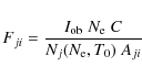
|
(1) |
calculated at a fixed temperature T0 and plotted as a function of the electron density
This approach is the same as analysing all the possible combinations of line ratios, as is commonly done in the literature. Departures from the isodensity or isothermal case can be important for some lines, but are normally second-order effects, compared to the uncertainties in the line identifications, line blending, instrument calibration, and in the atomic data. For Fe XI, the Fji curves have been calculated, unless otherwise stated, at log T0 [K] = 6.11, the approximate temperature of peak emission in ionization equilibrium (Dere et al. 2009).
The energy of the levels are then semi-empirically adjusted using the identified transitions.
The semi-empirical term energy correction (TEC) procedure (see, e.g. Zeippen et al. 1977;
Nussbaumer & Storey 1978) is adopted, to obtain empirically-adjusted fine-structure energies,
![]() .
For uncertain levels, the same corrections applied to other levels
having the same parent term are used at first. The adjusted
energies
.
For uncertain levels, the same corrections applied to other levels
having the same parent term are used at first. The adjusted
energies
![]() are then compared to the
observed energies
are then compared to the
observed energies
![]() ,
which are directly derived from the observed wavelengths
,
which are directly derived from the observed wavelengths
![]() .
Ground-based measurements have been converted to vacuum wavelengths
using the standard formula for the refractive index of air given by Edlén (1966).
.
Ground-based measurements have been converted to vacuum wavelengths
using the standard formula for the refractive index of air given by Edlén (1966).
The method was applied iteratively many times, before a suitable and
consistent set of energies and line intensities was obtained.
At the end of the iterative procedure, a set of experimental
energies
![]() is provided, from which experimental wavelengths
is provided, from which experimental wavelengths
![]() are obtained. Notice that occasionally, the
are obtained. Notice that occasionally, the
![]() values
can be slightly different from the observed ones. The final results
from the benchmark structure with and without TEC are presented in Del Zanna et al. (2010), along with the final scattering calculation. The experimental energies
values
can be slightly different from the observed ones. The final results
from the benchmark structure with and without TEC are presented in Del Zanna et al. (2010), along with the final scattering calculation. The experimental energies
![]() were then used to calculate the A-values
of all the E1, E2, M1, and M2 transitions in intermediate
coupling with AUTOSTRUCTURE using the same target used for the
scattering calculation.
were then used to calculate the A-values
of all the E1, E2, M1, and M2 transitions in intermediate
coupling with AUTOSTRUCTURE using the same target used for the
scattering calculation.
Table 1: Level energies for Fe XI.
4 Summary of results
The discussion is focused on the three main n=3 spectroscopic configurations in Fe XI, 3s2 3p4, 3s 3p5, 3s23p3 3d,
which produce 47 fine-structure levels, and all the brightest
lines for this ion. Additional levels from 3s 3p4 3d are also identified and briefly discussed. Table 1 lists the energies and identifications of the lowest 47 levels, together with a few from the 3s 3p4 3d configuration. The LS notation is ambiguous for many mixed levels. The experimental level energies
![]() (cm-1), together with those obtained from the scattering calculation
(cm-1), together with those obtained from the scattering calculation
![]() ,
and those from the National Institute of Standards and Technology (NIST) version 3 database
,
and those from the National Institute of Standards and Technology (NIST) version 3 database![]() are displayed. Most levels are now finally firmly established. The Fe XI energies presented here turn out to be very close to the ab-initio values obtained by Ishikawa & Vilkas (2008) using relativistic multi-reference many-body perturbation theory calculations, as shown in Del Zanna et al. (2010).
are displayed. Most levels are now finally firmly established. The Fe XI energies presented here turn out to be very close to the ab-initio values obtained by Ishikawa & Vilkas (2008) using relativistic multi-reference many-body perturbation theory calculations, as shown in Del Zanna et al. (2010).
Table 2 lists the
brightest lines (in decreasing order of intensity), grouped in
three wavelength ranges, EUV, UV, and UV/visible. The wavelengths
![]() corresponding to the experimental energies
corresponding to the experimental energies
![]() are shown, with gf and A values. The wavelengths
are shown, with gf and A values. The wavelengths
![]() obtained from the energies of the scattering calculation, and those from the NIST energies
obtained from the energies of the scattering calculation, and those from the NIST energies
![]() are also shown. Notice the large differences between
are also shown. Notice the large differences between
![]() and
and
![]() ,
which are however typical. Also, for many cases NIST wavelengths are close to
,
which are however typical. Also, for many cases NIST wavelengths are close to
![]() ,
although they are often significantly different, when high-resolution
observations such as those from Hinode/EIS are considered.
,
although they are often significantly different, when high-resolution
observations such as those from Hinode/EIS are considered.
It is very satisfactory to see that all the brightest transitions have been identified finally. Intensities were calculated at low (108 cm-3) and high (1012 cm-3) densities, typical of the quiet-Sun off-limb corona and of laboratory spectra. Notice the striking difference in the relative intensities of some lines, at different densities. The benchmark and identification using different sources took this into account.
A summary of the proposed identifications is given in Table 3. It lists the observed wavelengths
![]() that have been assessed to be best and used to obtain the experimental energies
that have been assessed to be best and used to obtain the experimental energies
![]() .
Some of the lines are self-blended or blend with transitions from other
ions. The most common ones are indicated in the table. However,
blending depends on the instrument resolution and on the plasma source.
The table also indicates some of the most relevant previous
identifications whether consistent or not with the present ones. The
reader should keep in mind that it is virtually impossible to provide
details for all the line identifications proposed, discussed, or
rejected in the literature.
.
Some of the lines are self-blended or blend with transitions from other
ions. The most common ones are indicated in the table. However,
blending depends on the instrument resolution and on the plasma source.
The table also indicates some of the most relevant previous
identifications whether consistent or not with the present ones. The
reader should keep in mind that it is virtually impossible to provide
details for all the line identifications proposed, discussed, or
rejected in the literature.
Table 2: List of the brightest Fe XI lines, from the EUV to the visible.
Table 3: Summary of line identifications for Fe XI.
5 Energy levels and line identifications
An in-depth discussion of the main spectral identifications for each of the levels is essential. In what follows, level energies are given in cm-1.
5.1 Ground configuration 3s2 3p4 and forbidden transitions
The splitting between the 3P
![]() levels is accurately measured by the 1-2 transition observed by Jefferies et al. (1971)
at 7891.8 Å (7894.0 Å in vacuum, which
provides 12 667.8). This is in good agreement with the
wavelength differences between decays from the same upper level to
levels 1, 2. For example, the decays from
level 37, observed at 188.216 and 192.813 Å,
provide an energy of 12 667.2. The energy of level 3 is
obtained from the wavelengths of the 3-44 and 2-44 lines observed
at 181.131 and 180.595 Å, and the energy
of level 2. The energy of level 4, 37 743,
is from the strong 1-4 transition observed by Sandlin et al. (1977) at 2648.71 Å (air). The wavelength of the 2-4 line observed by Jefferies et al. (1971) at 3986.8 Å (air) provides an energy of 37 743.6, in good agreement.
levels is accurately measured by the 1-2 transition observed by Jefferies et al. (1971)
at 7891.8 Å (7894.0 Å in vacuum, which
provides 12 667.8). This is in good agreement with the
wavelength differences between decays from the same upper level to
levels 1, 2. For example, the decays from
level 37, observed at 188.216 and 192.813 Å,
provide an energy of 12 667.2. The energy of level 3 is
obtained from the wavelengths of the 3-44 and 2-44 lines observed
at 181.131 and 180.595 Å, and the energy
of level 2. The energy of level 4, 37 743,
is from the strong 1-4 transition observed by Sandlin et al. (1977) at 2648.71 Å (air). The wavelength of the 2-4 line observed by Jefferies et al. (1971) at 3986.8 Å (air) provides an energy of 37 743.6, in good agreement.
The energy of level 5 is from the bright 2-5 line observed by Sandlin et al. (1977) at 1467.06 Å. Jordan (1971) used the 1970 eclipse observations described by Gabriel et al. (1971) to propose the identification of the 2-5 1467 Å line. Figure 4 shows the emissivity ratio of the 1467.06 Å line from the Sandlin et al. (1977) observation 40
![]() above an active region, together with those of new forbidden lines identified here, as described below.
above an active region, together with those of new forbidden lines identified here, as described below.
5.2 Transitions from the 3s 3p5 to the ground
Dipole-allowed decays from 3s 3p5 levels to the ground produce strong lines in the 300-370 Å range. These lines were identified for the first time using laboratory spectra by Fawcett (1971). The best spectra for the benchmark in terms of line intensities are those from the SERTS-89 and SERTS-97 rocket flights. Figure 5 shows the emissivity ratio curves, which agree to within 20% for all the lines known not to be blended. This confirms the accuracy of the scattering calculation for transitions to the 3s 3p5 levels.
An excellent ![]() -pinch calibrated spectrum was presented by Wang et al. (1984). Similarly, very good agreement in transitions from the 3s 3p5 levels is found when considering their laboratory spectrum, as shown in Fig. 6. This spectrum also provides good agreement with lines from the 3s2 3p33d configuration,
confirming the accuracy in the relative excitation rates between
transitions from these two configurations (and the
ground one).
-pinch calibrated spectrum was presented by Wang et al. (1984). Similarly, very good agreement in transitions from the 3s 3p5 levels is found when considering their laboratory spectrum, as shown in Fig. 6. This spectrum also provides good agreement with lines from the 3s2 3p33d configuration,
confirming the accuracy in the relative excitation rates between
transitions from these two configurations (and the
ground one).
The energy of level 6 is from the bright 1-6 observed by Be76 at 352.670 Å. Smitt et al. (1976) (hereafter S76) and TN94 measured 352.661 Å 352.672 Å respectively. This gives excellent agreement between predicted and observed wavelengths for the 2-6 transition observed by Be76 and TN94 at 369.161, 369.163 Å. S76 measured 369.154 Å, in slight disagreement. The energy of level 7 is from the strong 1-7 transition observed at 341.112, 341.113, 341.114 Å by Be76, S76, and TN94, respectively. Notice that the strong 3-7 and 2-7 transitions are predicted to be at 358.613 Å and 356.519 Å respectively. Also notice that S76 measured 358.621 Å and 356.519 Å in laboratory spectra, and that both lines are blended in solar spectra. The energy of level 8 is from the weak 2-8 transition measured by S76 at 349.046 Å. This transition is severely blended with lines from Mg VI in solar spectra.
The energy of level 9 (which is highly mixed) is tentatively assigned by adopting the Be76 wavelength of 308.544 Å for the 4-9 transitions, noting that this line is likely blended. Indeed TN94 in their active region spectrum measure a line with a different wavelength, 308.575 Å. The MR-RP energies predict 308.71 Å, while Jupén et al. (1993) identified the 4-9 with the 308.515 Å line in their laboratory spectra. S76 identified instead the 5-9 transition with a laboratory line observed at 355.837 Å. An energy of 361 859 would follow, and a wavelength of 308.532 Å for the 4-9 transition is predicted, not too far from the Be76 wavelength.
![\begin{figure}
\par\includegraphics[angle=90,width=16.5cm,clip]{H14063f3.ps}
\end{figure}](/articles/aa/full_html/2010/06/aa14063-10/img25.png)
|
Figure 3: Sections of the Hinode EIS off-limb spectrum used to benchmark Fe XI (units are averaged counts per pixel). |
| Open with DEXTER | |
5.3 Transitions from the 3s2 3p33d configuration to the ground
Dipole-allowed decays from 3s2 3p33d levels to the ground produce the brightest Fe XI lines, visible in the EUV in the 160-260 Å range (see Table 2). Several lines were first identified by Gabriel et al. (1966). More identifications were provided by Bromage et al. (1977); however, many subsequent authors have provided differing identifications (e.g. Jupén et al. 1993; Träbert 1998).
5.3.1 3s2 3p3 (4S) 3d 5D
 (levels 10-14)
These levels are relatively pure. As shown by Träbert (1998, and references therein), the transition array 3s2 3p4 3P
![]() -3s2 3p3 3d 5D
-3s2 3p3 3d 5D
![]() produces two groups of lines that are strong in the
delayed beam-foil spectra. The first group consists of transitions to the J=2 ground state and is observed around 257 Å. The second group consists of decays to the J=0,1 levels, and is observed
around 266 Å. In astrophysical conditions, our calculations predict that the strongest decays from the 3s2 3p3 3d 5D
produces two groups of lines that are strong in the
delayed beam-foil spectra. The first group consists of transitions to the J=2 ground state and is observed around 257 Å. The second group consists of decays to the J=0,1 levels, and is observed
around 266 Å. In astrophysical conditions, our calculations predict that the strongest decays from the 3s2 3p3 3d 5D
![]() levels are the 1-14, 1-13, 1-12, and 1-11, in order of
decreasing intensity. The beam-foil spectra are very important because
they provide a tight constraint on the possible energies of the 3s2 3p3 3d 5D
levels are the 1-14, 1-13, 1-12, and 1-11, in order of
decreasing intensity. The beam-foil spectra are very important because
they provide a tight constraint on the possible energies of the 3s2 3p3 3d 5D
![]() levels, although the spectral resolution is such that wavelengths are only known with an accuracy of 1-2 Å.
levels, although the spectral resolution is such that wavelengths are only known with an accuracy of 1-2 Å.
![\begin{figure}
\par\includegraphics[angle=90,width=8.5cm,clip]{H14063f4.ps}
\end{figure}](/articles/aa/full_html/2010/06/aa14063-10/img28.png)
|
Figure 4:
The emissivity ratio curves from the Skylab ATM observation 40
|
| Open with DEXTER | |
In the first group of transitions, Träbert (1998)
tentatively identified the 1-13, 1-12, and 1-11 transitions with
the lines observed at 257.26, 257.55, 257.78 Å, respectively.
Different identifications are provided here, mainly based on the
Hinode/EIS observations as described below. Regarding the second group
of transitions, Träbert (1998) tentatively
identified the 2-12, 2-11, and 2-10 with the lines observed
at 266.23, 266.42, and 266.60 Å.
These lines are predicted to be extremely weak in solar spectra and
might actually not be observable. The energy of level 10 is
therefore very difficult to assign accurately. However, using the the
firm identifications of the other 5D
![]() levels
and their theoretical splittings (see below), a wavelength
of 266.74 Å for the 2-10 transition is predicted. This
transition is tentatively assigned to a weak line observed with
Hinode/EIS at 266.755 Å, with a wavelength still consistent with
the beam-foil measurements. The tentative identification by Träbert (1998) is therefore ruled out.
levels
and their theoretical splittings (see below), a wavelength
of 266.74 Å for the 2-10 transition is predicted. This
transition is tentatively assigned to a weak line observed with
Hinode/EIS at 266.755 Å, with a wavelength still consistent with
the beam-foil measurements. The tentative identification by Träbert (1998) is therefore ruled out.
![\begin{figure}
\par\includegraphics[angle=90,width=8.5cm,clip]{H14063f5a.ps}\par\includegraphics[angle=90,width=8.5cm,clip]{H14063f5b.ps}
\end{figure}](/articles/aa/full_html/2010/06/aa14063-10/img29.png)
|
Figure 5: Emissivity ratio curves relative to the SERTS-89 and SERTS-97 calibrated data. |
| Open with DEXTER | |
![\begin{figure}
\par\includegraphics[angle=90,width=8.5cm,clip]{H14063f6.ps}
\end{figure}](/articles/aa/full_html/2010/06/aa14063-10/img30.png)
|
Figure 6:
Emissivity ratio curves relative to the laboratory spectrum of Wang et al. (1984).
|
| Open with DEXTER | |
The energy of level 11 is assigned from the weak 1-11 transition, which is identified here with the Hinode/EIS line at 257.914 Å. This new energy predicts a wavelength of 266.63 Å for the 2-11 transition, which is different from (though very close to) the suggested value of 266.42 Å given by Träbert (1998). The energy of level 12 is obtained by assigning the observed wavelength of 257.772 Å to the 1-12 transition. This agrees with the identification given by Jupén et al. (1993). We find excellent agreement between the Be76 and Hinode/EIS wavelength. The new energy predicts a wavelength of 266.47 Å for the 2-12 transition, which is different from (though very close to) the suggested value of 266.23 Å given by Träbert (1998). Similarly, the energy of level 13 is obtained by assigning the observed wavelength of 257.55 Å to the 1-13 transition, in agreement with the identification given by Jupén et al. (1993). However, this line is actually a close self-blend with the 4-20 transition (see below). The wavelength given by Be76 is 257.547 Å, which provides an energy of 388 279. The actual energy chosen here is 388 268, based on 4 new identifications of strong UV lines that form two branching ratios, the 14-25 vs. 13-25 and the 14-32 vs. the 13-32 line (see below).
The model ion predicts a strong decay to the ground state from level 14, observable by Hinode/EIS. It is identified here with the strong line observed by EIS at 256.925 Å. However, the energy of this level is obtained from the new identification of the 6-14 transition, observed by SOHO/SUMER at 946.29. The energy of level 14 provides a wavelength for the decay to the ground of 256.920 Å, close to the EIS value. The energy agrees with the observed wavelength of the 14-32 UV transition, as described below. Be76 also reports 256.925 Å, but gives a tentative identification as an unspecified Fe XV transition. In reality, current atomic models for Fe XV do not predict any strong line due to this ion around these wavelengths. Also, in the EIS off-limb quiet-Sun spectra there is almost no Fe XV emission, so any blending with this ion can be ruled out. Del Zanna & Mason (2005) tentatively identified a level in Fe XII that would provide a weak transition around 256.93 Å. However, the Fe XII atomic data predict that this line would only be 2-3% the intensity of this strong transition for the Hinode/EIS spectrum considered here. Indeed, the predicted intensity is within the observed one, as Fig. 7 (top right) shows.
The decays from the 3s2 3p3 3d 5D
![]() levels
are particularly important because they provide a direct temperature
diagnostic, when observed in combination with any of the other lines
from higher levels, as shown in Fig. 7 (top left). To within 30%, the observed lines indicate an isothermal electron temperature of
levels
are particularly important because they provide a direct temperature
diagnostic, when observed in combination with any of the other lines
from higher levels, as shown in Fig. 7 (top left). To within 30%, the observed lines indicate an isothermal electron temperature of ![]() [K] = 5.8,
perhaps lower than expected. The absolute value depends on the relative
calibration between the two EIS channels which is not well established.
The lines presented in Fig. 7
(top left) depend very little
from the electron density, so the resulting temperature does not
depend on the density. On the other hand, many of the lines discussed
in this section have some temperature dependence. The value of
[K] = 5.8,
perhaps lower than expected. The absolute value depends on the relative
calibration between the two EIS channels which is not well established.
The lines presented in Fig. 7
(top left) depend very little
from the electron density, so the resulting temperature does not
depend on the density. On the other hand, many of the lines discussed
in this section have some temperature dependence. The value of ![]() [K] = 5.8
was used for the emissivity ratio curves (as a function of
density) for the other lines shown in Fig. 7. Larger discrepancies are found in general if a temperature close to
[K] = 5.8
was used for the emissivity ratio curves (as a function of
density) for the other lines shown in Fig. 7. Larger discrepancies are found in general if a temperature close to ![]() [K] = 6.11 is used.
[K] = 6.11 is used.
![\begin{figure}
\par\includegraphics[angle=90,width=7cm,clip]{H14063f7a.ps}\hspac...
...ace*{5mm}
\includegraphics[angle=90,width=7.5cm,clip]{H14063f7d.ps}
\end{figure}](/articles/aa/full_html/2010/06/aa14063-10/img32.png)
|
Figure 7: Emissivity ratio curves for a selection of lines from the Hinode EIS off-limb spectrum. In the top left, the curves are shown as a function of the electron temperature, the others as a function of density. The top right plot shows the curves for the brightest lines, while the others include the weaker ones, in the SW and LW channels. |
| Open with DEXTER | |
5.3.2 3s2 3p3 (2D) 3d 3D
(levels 15-17)
The 15-17 are highly mixed levels. The model ion predicts that two decays from level 16 should be observable. That one to the ground state is not visible by Hinode/EIS, but the 4-16 should be an observable line. A search through possible wavelength coincidences produces only one result: the 1-16 transition should be blended with Fe XIII in the line observed at 240.713 Å by Hinode/EIS, while the 4-16 line would be blended with a strong Fe XIV line observed at 264.787 Å. That the 240.713 Å line is blended is confirmed by two facts. First, Be76 indicate that the line is a blend, and TN94 report a very broad line, with 0.102 Å FWHM. Second, the Fe XIII benchmark (work in progress) indicates that about half of the intensity of this line does not come from Fe XIII. The new identification (see below) of the 1408.70 Å line with the 16-32 transition provides an accurate energy for level 16 of 415 426, which results in a wavelength of 240.717 Å, which is only 4 mÅ from the observed blend.
Levels 15 and 17 are more difficult to establish. The 1-15 transition should be well observable. Based on the differences between theoretical and observed energies of the other levels, this transition is predicted to be at 242.2 Å. Be76 measured an unidentified line at 242.215 Å, so we identify it with the 1-15 transition, although its observed intensity is about twice the predicted one. This predicts that a weak but observable 4-15 line by EIS should fall at 266.586 Å. There is an unidentified line, with about the right intensity, but at 266.613 Å. The same arguments apply to level 17, with a decay to the ground state predicted to have a wavelength of 239.75 Å. This line should be much weaker than the 1-15, so it is likely to be either the 239.52 Å observed by Behring et al. (1976) or the 239.78 Å observed by Dere (1978). We tentatively assign it to the latter.
5.3.3 3s2 3p3 (2D) 3d 3F
(levels 18, 20, 21)
Levels 18, 20, 21 are relatively pure. The energy of the important metastable level 21 is obtained here from the Be76 measurement of the previously-unidentified line at 254.596 Å with the strong 4-21 transition. The Hinode/EIS wavelength is 254.600 Å. This is a new identification. The new energy for this level predicts that the strong 6-21 transition would be at 680.40 Å. There is indeed a strong, previously unidentified, coronal line blending a line observed by SUMER at 680.28 Å. The forbidden 14-21 transition is predicted to have a wavelength of 2423 Å (vacuum), and it was too weak to be observed by Sandlin et al. (1977).
![\begin{figure}
\par\includegraphics[angle=90,width=12cm,clip]{H14063f8.ps}
\end{figure}](/articles/aa/full_html/2010/06/aa14063-10/img33.png)
|
Figure 8: The emissivity ratio curves relative to the full-Sun spectrum of Malinovsky & Heroux (1973). Lines deblended (dbl) and blended (bl, sbl) are indicated. Those with a * were not published and have a large (30-50%) uncertainty. Lines newly identified are indicated by N. |
| Open with DEXTER | |
The energy of level 20 is obtained from the following considerations. The theoretical splitting with level 21 predicts that a weak but observable line should be present around 257.51 Å. The transitions 4-20 and 1-20 are predicted to be weak, however the 4-20 in particular should be observable with EIS. If we identify it as blending (with the 1-13) the line observed at 257.547 Å, we obtain a wavelength for the decay to the ground state of 234.73 Å, which coincides with a line reported as Fe XV by Dere (1978). To support this, it appears unlikely that the 234.73 Å line comes from Fe XV. The Fe XV 3s 3p 3P2-3s 3d 3D2 line is in fact predicted to be more than ten times weaker than the 3s 3p 1P1-3s 3d 1D2 transition observed at 243.78 Å, while the observed intensity is approximately half or more (if blending with Ar XV in the 243.78 Å line is considered).
Having established the energies of the other levels, it becomes easier to find the energy of level 18. Theoretical splittings predict that an observable line should fall around 236.5 Å. Indeed there is an unidentified line in the Be76 spectrum at 236.494 Å.
5.3.4 3s2 3p3 (2D) 3d 3G
(levels 22-24)
Levels 22-24 are relatively pure. The energy of the important metastable level 24 is obtained from the 14-24 transition, which is identified here as the coronal line observed by Sandlin et al. (1977) at 1582.56 Å and from the new energy of the level 14. Excellent agreement in terms of line intensity is found, as shown in Fig. 4. Sandlin et al. (1977) gave a tentative identification as Ar XIII for this line. The new energy predicts an air wavelength of 4566.2 Å for the strong 21-24 transition, exactly the same value measured by Jefferies et al. (1971). Mason & Nussbaumer (1977) originally suggested this identification. Feldman & Doschek (1977) incorrectly identified the coronal line at 1582.6 Å with an Fe X transition. As shown by Del Zanna et al. (2004), the Fe X transition was predicted to be more than two orders of magnitude weaker than the observed line.
The energy of the important metastable level 23 is obtained as
follows. Having established the energy of level 24, the
theoretical splitting between levels 23 and 24 predicts that
a relatively strong 14-23 transition should be observed around
1639 Å. Indeed, Sandlin et al. (1977)
reported a line observed at 1639.78 ![]() 0.03 Å, identified by them as the O VII 1s 2s 3S1-1s 2p 3P0 transition. This transition, however, is predicted to be 5 times weaker than the 1s 2s 3S1-1s 2p 3P2 transition observed by Sandlin et al. (1977) at 1623.54 Å. In their actual off-limb spectra, the 1639.78 Å line was instead more than twice as
strong as the 1623.54 Å line. The 14-23 transition is therefore identified as blending the O VII 1s 2s 3S1-1s 2p 3P0 line. Actually, in the off-limb spectrum, it appears that the observed line is entirely due to Fe XI, as shown in Fig. 4. The decay 13-23 is predicted to be 10 times weaker, at 1614.39 Å, possibly blending the S XI measured at 1614.51 Å by Sandlin et al. (1977).
0.03 Å, identified by them as the O VII 1s 2s 3S1-1s 2p 3P0 transition. This transition, however, is predicted to be 5 times weaker than the 1s 2s 3S1-1s 2p 3P2 transition observed by Sandlin et al. (1977) at 1623.54 Å. In their actual off-limb spectra, the 1639.78 Å line was instead more than twice as
strong as the 1623.54 Å line. The 14-23 transition is therefore identified as blending the O VII 1s 2s 3S1-1s 2p 3P0 line. Actually, in the off-limb spectrum, it appears that the observed line is entirely due to Fe XI, as shown in Fig. 4. The decay 13-23 is predicted to be 10 times weaker, at 1614.39 Å, possibly blending the S XI measured at 1614.51 Å by Sandlin et al. (1977).
5.3.5 Level 25
The energy of the important metastable level 25 is obtained from
the 14-25 transition, which is identified here for the first time
as the strong coronal line, observed by Sandlin et al. (1977) at 1428.75 ![]() 0.01 Å. Excellent agreement between predicted and observed intensity is found, as shown in Fig. 4. The same line is prominent in SOHO/SUMER spectra at the same wavelength (Feldman et al. 1997). This allows another new identification: the strong 13-25 transition with the line observed by Sandlin et al. (1977) (and also by Feldman et al. 1997) at 1409.45
0.01 Å. Excellent agreement between predicted and observed intensity is found, as shown in Fig. 4. The same line is prominent in SOHO/SUMER spectra at the same wavelength (Feldman et al. 1997). This allows another new identification: the strong 13-25 transition with the line observed by Sandlin et al. (1977) (and also by Feldman et al. 1997) at 1409.45 ![]() 0.01 Å. This wavelength is used to obtain the energy of
level 13, 388 268. The observed intensity is in good
agreement with the predicted one also in this case, as Fig. 4 shows.
0.01 Å. This wavelength is used to obtain the energy of
level 13, 388 268. The observed intensity is in good
agreement with the predicted one also in this case, as Fig. 4 shows.
5.3.6 3s2 3p3 (2P) 3d 3P
(levels 28, 29, 34)
Levels 28, 29, and 34 are relatively pure. The strongest decay is the 1-34 transition. We identify it as the (previously unknown) 202.424 Å line in the Behring et al. (1976) spectrum. The EIS wavelength is very close, 202.426 Å. The weaker 2-34 transition is therefore predicted to be at 207.751 Å. Indeed a weak line in the Hinode EIS spectra is observed at 207.749 Å.
The 3s2 3p3 (2P) 3d 3P
![]() (29)
is predicted to produce a decay to the ground state also observable by
Hinode/EIS. An inspection of the EIS spectra shows that this
transition can only be one of the lines observed at 206.166,
206.258, 206.365 Å with EIS. The Be76 measurements are
consistent (206.169, 206.253, 206.369 Å). The latter is a weak Fe XII transition according to the Del Zanna & Mason (2005) model ion. Various authors (e.g. Brown et al. 2008) identify the 206.258 Å line with the (strong in relative terms) 2s2 1S0-2s 2p 1P1 resonance line from K XVI
at 206.253 Å; however,
this cannot be, given that the peak abundance in ionization equilibrium
for this ion is 5 MK, far too high for any quiet Sun plasma.
The 1-29 transition is identified here with the
206.258 Å line, considering that the 206.166 Å line
is assigned to the 1-30 (see below).
(29)
is predicted to produce a decay to the ground state also observable by
Hinode/EIS. An inspection of the EIS spectra shows that this
transition can only be one of the lines observed at 206.166,
206.258, 206.365 Å with EIS. The Be76 measurements are
consistent (206.169, 206.253, 206.369 Å). The latter is a weak Fe XII transition according to the Del Zanna & Mason (2005) model ion. Various authors (e.g. Brown et al. 2008) identify the 206.258 Å line with the (strong in relative terms) 2s2 1S0-2s 2p 1P1 resonance line from K XVI
at 206.253 Å; however,
this cannot be, given that the peak abundance in ionization equilibrium
for this ion is 5 MK, far too high for any quiet Sun plasma.
The 1-29 transition is identified here with the
206.258 Å line, considering that the 206.166 Å line
is assigned to the 1-30 (see below).
5.3.7 3s2 3p3 (2P) 3d 3F
(levels 30-32)
Among the levels 30-32, the middle one is significantly mixed and does not produce any strong transitions, so that it remains unidentified. Level 32 is a metastable level, so is important because it produces strong forbidden lines in the UV. The calculations show that a strong 14-32 line should be present in the SUMER spectra. We identify it with the (previously unidentified) coronal line observed by Feldman et al. (1997) at 1028.95 Å (with a possible additional blend). This provides an energy for level 32 of 486 413 (using the new energy for level 14 of 389 227).
The line observed by SOHO/SUMER at 1018.89 Å cannot be the Ar XII 2s2 2p3 4S3/2-2s2 2p3 2D5/2 transition as identified by Feldman et al. (1997), considering that it is much brighter than the 2s2 2p3 4S3/2-2s2 2p3 2D3/2 (observed at 1054.57 Å), the opposite of what it should be. Its morphology suggests that it is a strong coronal line. It is identified here as the Fe XI 13-32 transition (possibly slightly blended with Ar XII). This provides the energy of level 13.
The energy of level 32 also provides an accurate energy for level 16. The 16-32 line is predicted to be about 1/2 of the intensity of the 13-25 transition. The 16-32 line is identified here with the line observed by SOHO/SUMER at 1408.70 Å (Feldman et al. 1997), based on wavelength and intensity arguments. Excellent agreement between predicted and observed intensity is found, as shown in Fig. 4.
Having established the energy of level 32, it becomes easier to find the energy of level 30, considering the theoretical splitting between the two levels. A weak 1-30 transition should be observable by Hinode/EIS, and indeed a line with the right wavelength and intensity is found at 206.166 Å. The Be76 measurement of 206.169 Å is chosen to establish the energy of level 30.
5.3.8 3s2 3p3 (2P) 3d 3D
(levels 27, 33, 35)
Levels 27, 33, and 35 are mixed, in particular the middle one. The strongest transition is the 1-35, predicted to be around 201 Å. When considering its intensity, the only possibility is that this transition is blending a much stronger Fe XIII line. The blend is at 201.112 Å as measured by Hinode/EIS. The line is slightly broader than the others, which also confirms blending. Be76 measured 201.121 Å but indicated a blend with a second-order line. Having established level 35, it follows that level 33 should produce a transition (2-33) observable by Hinode/EIS around 209.8 Å. Indeed an unidentified line at 209.771 Å is observed, and this wavelength is used to establish the energy of level 33. Level 27 remains unknown, given that it produces a weak 3-27 transition around 214 Å, not observable by Hinode/EIS.
5.3.9 Level 36
The weak 1-36 transition is identified here with a blend observed by Hinode/EIS at 190.382 Å. Various authors (e.g. Be76, Brown et al. 2008) have previously identified a line observed around 190.4 Å with the S XI 2s2 2p2 1D2-2s 2p3 1P1, which has a different wavelength of 190.355 Å, according to NIST. Be76 measured it at 190.372 Å. This transition cannot be clearly due to S XI for three reasons. First, this ion emits around 2 MK, too high a temperature for the quiet Sun. Second, the intensity of this transition is predicted to be only about 3% of the intensity of the S XI 2s2 2p2 3P1-2s 2p3 3S1 188.675 Å, which is observed in the off-limb EIS spectrum at 188.673 Å to be very weak. Third, its wavelength does not coincide with the NIST wavelength for S XI.
5.3.10 Levels 37-41
A detailed account of the complexities in establishing the identifications of these levels is provided in Del Zanna et al. (2010). The energy of level 38 is obtained from the strong 1-38 transition, observed by Be76 at 188.216 Å. The energy of level 37 is obtained from the strong 1-37 transition, observed by Be76 at 188.299 Å. The level has another strong decay (4-37) with a predicted wavelength of 202.706 Å, in good agreement with the observed one by Behring et al. (1976) and Hinode/EIS of 202.710 Å. The 2-37 transition is particularly important because it blends the resonance line of Ca XVII, together with other transitions, mostly from O V. The off-limb Hinode/EIS spectrum is particularly good because all cooler emission is absent, so this line should mainly come from Fe XI. In reality, as Fig. 7 shows, this line still appears to be blended. The line is predicted at 192.813 Å and observed at 192.811 Å, in excellent agreement.
The 1-37 line has been the subject of much confusion and controversy, as reviewed in Del Zanna et al. (2010), with conflicting identifications and very different gf values. It is therefore important to assess whether the new scattering calculations provide good agreement with observations. The best observation is by Malinovsky & Heroux (1973), although the 1-37 was blended with the 1-38 transition in that spectrum. The agreement between the self-blend 1-38 + 1-37 and the other strong lines (1-43, 1-42, 2-44, 3-44) in the Malinovsky & Heroux (1973) observation is excellent (to within 10%). This result shows that the new scattering calculation is very accurate, because it predicts a correct intensity (to within 10%) for the self-blend 1-38 + 1-37. Large discrepancies are present if any other scattering calculation is adopted. Hinode/EIS does resolve the 1-38 and 1-37 lines, and good agreement (to within 10%) is found in the relative intensities of these two lines, as shown in Fig. 7. These lines are the strongest ones after those of Fe XII in EIS spectra (cf. Fig. 3).
The energy of level 39 is difficult to establish accurately, given that all the decays are weak and blended to some degree. The strongest decay is the 4-39 transition, blended (by about 10%) with an Fe XII line (Del Zanna & Mason 2005), and observed by Be76 at 201.734 Å, in agreement with the Hinode/EIS wavelength of 201.737 Å. We used the 201.734 Å value to obtain the energy. This predicts that the decay to the ground state should be observed at 187.461 Å. In the Hinode/EIS observation, a weak line is observed at 187.437 Å, which is presumably the 1-39 (blended). The 2-39 transition is predicted at 192.021 Å, and indeed Hinode/EIS observes a weak line exactly at 192.021 Å with about the expected intensity. This line in on-disk observations is strongly blended with Fe VIII and other unidentified cool emission (Del Zanna 2009b,a), and also in flaring conditions with the strong Fe XXIV 192.028 Å. The 3-39 transition is predicted at 192.627 Å. Hinode/EIS observes a line at the right wavelength, 192.624 Å, but the model predicts that only about 1/2 of the intensity comes from Fe XI.
Level 40 only has one one dipole-allowed transition to the ground configuration, the 2-40 transition, identified with the line observed at 188.997 Å by Behring et al. (1976) (and at 189.005 Å with Hinode/EIS). Level 41 is difficult to establish because it produces various weak decays, all of which appear to be blended to some degree (see Fig. 7). The strongest one is the 4-41 line, which is blended with a strong S VIII transition observed at 198.552 Å by Hinode/EIS. Be76 incorrectly identifies the line as blended with Fe XII. The second strongest line is the 2-41, observed by Hinode/EIS at 189.121 Å. This line appears to be slightly blended. The Be76 wavelength of 189.123 Å is chosen to establish the energy of this level. This predicts the 4-41 to be at 198.539 Å, and the weaker 3-41 transition at 189.712 Å. Hinode/EIS observes a (broad) line at a close wavelength, 189.723 Å, but slightly brighter than expected, an indication of a blend here. Be76 gives a slightly longer wavelength, 189.733 Å. The very weak 1-41 is then predicted at 184.698 Å, a wavelength too far from the line observed by Hinode/EIS at 184.796 Å (Be76 gives 184.793 Å) and identified as the 4-45 (see below). Hinode/EIS does observe some emission at 184.70 Å with the correct intensity, although it is too weak to produce a clean line profile.
5.3.11 Levels 42-48
The energy of level 42 is from the strong 1-42 line, observed at 180.401 Å by Be76. This line is slightly blended with Fe X (Paper I) and Fe XII. The energy of level 43 is from the strong 2-43 transition observed at 182.167 Å by Be76. This predicts the 1-43 line at 178.058 Å, in excellent agreement with the observed value (178.056 Å). Hinode/EIS wavelengths are within a few mÅ.
The energy of level 44 is provided from the wavelengths of the 3-44 and 2-44 lines, 181.131 Å and 180.595 Å. The energy of level 45 is obtained from the weak 4-45 line, observed at 184.793 Å by Be76 (184.796 Å by Hinode/EIS). The energy of level 46 is obtained from the weak 4-46 line, observed at 179.758 Å by Be76. The Hinode/EIS wavelength is slightly lower (179.742 Å). The 4-45 and 4-46 lines are very strong in laboratory spectra, with wavelengths that confirm those of Be76 (B.C. Fawcett, plate C50, priv. comm.).
The energy of level 47 is provided from the wavelength of the
5-47 line, strong only in laboratory spectra. This line is very
close to the strong Fe X (Paper I) line, measured by Be76 at 184.536 Å ![]() 0.002 Å.
The wavelength measurements in second order of plate C50 (B.C. Fawcett,
priv. comm.) of these two close lines provide a wavelength of
184.410 Å
0.002 Å.
The wavelength measurements in second order of plate C50 (B.C. Fawcett,
priv. comm.) of these two close lines provide a wavelength of
184.410 Å ![]() 0.002 Å, which is adopted here. Hinode/EIS observes a weak line at
184.413 Å, but its intensity is higher than predicted.
0.002 Å, which is adopted here. Hinode/EIS observes a weak line at
184.413 Å, but its intensity is higher than predicted.
Finally, the ratios of the strong lines 2-43, 3-44 with
e.g. the 1-42 is a well-known and very good electron density
diagnostic. The curves form the Malinovsky & Heroux (1973) observation
indicate an electron density log ![]() = 8.5 cm-3, in excellent agreement with the values derived from other ions such as Fe XII (Storey et al. 2005; Del Zanna & Mason 2005).
Good agreement is also found in Hinode/EIS spectra, although the
strongest line, the 1-42 180.40 Å, consistently has an
observed intensity that is too low by a 20% or so
(cf. Fig. 7). This can only be due to an incorrect radiometric calibration around 180 Å.
= 8.5 cm-3, in excellent agreement with the values derived from other ions such as Fe XII (Storey et al. 2005; Del Zanna & Mason 2005).
Good agreement is also found in Hinode/EIS spectra, although the
strongest line, the 1-42 180.40 Å, consistently has an
observed intensity that is too low by a 20% or so
(cf. Fig. 7). This can only be due to an incorrect radiometric calibration around 180 Å.
5.4 Transitions from 3s 3p4 3d
The decays from the 3s 3p4 3d configuration are predicted to be weak. The strongest transitions are the 16-67, 21-79, 6-103, and 14-54. The strongest is the 16-67, which should be observable and around 310 Å. An accurate search, which involves comparing observed and predicted line intensities in a 10 Å window, leaves only one possibility, that this is the previously unidentified line in the SERTS-97 active region spectrum (Brosius et al. 2000) at 308.991 Å. Lines above 310 Å are excluded by considering quiet-Sun off-limb SOHO/CDS spectra. No strong unidentified lines are present, and there were no indications of significant blending (Del Zanna 1999). The 4-9 transition only accounts for about 1/2 of the intensity of the observed line, in the SERTS-89 spectrum, however its intensity agrees well with the other lines in the SERTS-97 spectrum (see Fig. 5). The intensities of the 4-9 and 16-67 are predicted to be similar, and no other line is present. The energy difference between the experimental and target energies for level 67 is only 2185 cm-1.
The second transition, 21-79, is predicted to be observable by Hinode/EIS. A similar adjustment to the target energies of all the levels in the 3s2 3p3 3d configuration predicts a line around 267 Å. The only reasonable candidate with the correct wavelength and intensity is the weak line observed at 266.755 Å with Hinode/EIS. The difference between predicted and observed energies is only 1740 cm-1.
The weak 6-103 transition could either be blended with the weak Fe VIII 168.929 Å or be the weak unidentified line at 169.614 Å in the Be76 spectrum. Preference is given to the first choice on energy grounds. The weak 14-54 transition is predicted to be about 1/10 the intensity of the 1-7 341.113 Å line at low densities and have a wavelength close to 327 Å. There is only one previously unidentified transition, observed by SOHO/CDS in quiet-Sun off-limb spectra at 326.3 Å, as discussed in Del Zanna (1999). The SERTS-97 wavelength of 326.323 Å is adopted.
6 Summary and conclusions
A comprehensive benchmark of Fe XI atomic data against available observations has been presented. All previous line identifications were reviewed by comprehensively comparing the results of the new scattering and structure calculations with experimental data. The results indicate that the new atomic model is accurate to within 10% for all the strongest transitions, a remarkable result considering the difficulty obtaining a good target for this ion.
Several new levels and transitions have been identified at last, opening the possibility of further identifications along the S I-like sequence, as described in a follow-up paper. The assessment indicates the presence of many blends.
A number of strong lines can now be used to measure electron density reliably. Also, it is shown here for the first time that a few transitions can be used to measure electron temperatures. For the Hinode/EIS wavelengths, Fe XI offers the best diagnostic for coronal temperatures. For lower temperatures, the best diagnostics are from Fe VII and Fe VIII, as described in Del Zanna (2009a) and Del Zanna (2009b). It is recommended that future Hinode/EIS observing sequences include these lines, and that a thorough radiometric calibration programme is put in place in the near future so reliable measurements can be obtained.
The support from STFC (Advanced Fellowship and APAP-network) is acknowledged. I warmly thank B.C. Fawcett for continuous support and encouragement, and for many exchanges of correspondence over the years. E. Träbert (Bochum and Livermore) is also thanked for useful exchanges of information. Hinode is a Japanese mission developed and launched by ISAS/JAXA, with NAOJ as the domestic partner and NASA and STFC (UK) as international partners. It is operated by these agencies in co-operation with ESA and NSC (Norway).
References
- Badnell, N. R. 1997, J. Phys. B Atom. Mol. Phys., 30, 1 [Google Scholar]
- Behring, W. E., Cohen, L., & Feldman, U. 1972, ApJ, 175, 493 [NASA ADS] [CrossRef] [Google Scholar]
- Behring, W. E., Cohen, L., Doschek, G. A., & Feldman, U. 1976, ApJ, 203, 521 [NASA ADS] [CrossRef] [Google Scholar]
- Bromage, G. E., Cowan, R. D., & Fawcett, B. C. 1977, Phys. Scr, 15, 177 [Google Scholar]
- Brosius, J. W., Davila, J. M., & Thomas, R. J. 1998a, ApJ, 497, L113 [NASA ADS] [CrossRef] [Google Scholar]
- Brosius, J. W., Davila, J. M., & Thomas, R. J. 1998b, ApJS, 119, 255 [NASA ADS] [CrossRef] [Google Scholar]
- Brosius, J. W., Thomas, R. J., Davila, J. M., & Landi, E. 2000, ApJ, 543, 1016 [NASA ADS] [CrossRef] [Google Scholar]
- Brown, C. M., Feldman, U., Seely, J. F., Korendyke, C. M., & Hara, H. 2008, ApJS, 176, 511 [NASA ADS] [CrossRef] [Google Scholar]
- Culhane, J. L., Harra, L. K., James, A. M., et al. 2007, Sol. Phys., 60 [Google Scholar]
- Del Zanna, G. 1999, Ph.D. Thesis, Univ. of Central Lancashire, UK [Google Scholar]
- Del Zanna, G. 2009a, A&A, 508, 501 [NASA ADS] [CrossRef] [EDP Sciences] [Google Scholar]
- Del Zanna, G. 2009b, A&A, 508, 513 [NASA ADS] [CrossRef] [EDP Sciences] [Google Scholar]
- Del Zanna, G., & Ishikawa, Y. 2009, A&A, 508, 1517 [NASA ADS] [CrossRef] [EDP Sciences] [Google Scholar]
- Del Zanna, G., & Mason, H. E. 2005, A&A, 433, 731 [NASA ADS] [CrossRef] [EDP Sciences] [Google Scholar]
- Del Zanna, G., Bromage, B. J. I., Landi, E., & Landini, M. 2001, A&A, 379, 708 [NASA ADS] [CrossRef] [EDP Sciences] [Google Scholar]
- Del Zanna, G., Berrington, K. A., & Mason, H. E. 2004, A&A, 422, 731 [NASA ADS] [CrossRef] [EDP Sciences] [Google Scholar]
- Del Zanna, G., Storey, P. J., & Mason, H. E. 2010, A&A, 514, A40 [NASA ADS] [CrossRef] [EDP Sciences] [Google Scholar]
- Dere, K. P. 1978, ApJ, 221, 1062 [NASA ADS] [CrossRef] [Google Scholar]
- Dere, K. P., Landi, E., Young, P. R., et al. 2009, A&A, 498, 915 [NASA ADS] [CrossRef] [EDP Sciences] [Google Scholar]
- Edlén, B. 1966, Metrologia, 2, 71 [NASA ADS] [CrossRef] [Google Scholar]
- Eissner, W., Jones, M., & Nussbaumer, H. 1974, Comput. Phys. Commun., 8, 270 [NASA ADS] [CrossRef] [Google Scholar]
- Fawcett, B. C. 1970, J. Phys. B Atom. Mol. Phys., 3, 1732 [NASA ADS] [CrossRef] [Google Scholar]
- Fawcett, B. C. 1971, J. Phys. B Atom. Mol. Phys., 4, 1577 [Google Scholar]
- Fawcett, B. C., Gabriel, A. H., & Saunders, P. A. H. 1967, Proc. Phys. Soc., 89, 863 [NASA ADS] [CrossRef] [Google Scholar]
- Feldman, U., & Doschek, G. A. 1977, J. Opt. Soc. Am., 67, 726 [NASA ADS] [CrossRef] [Google Scholar]
- Feldman, U., Behring, W. E., Curdt, W., et al. 1997, ApJS, 113, 195 [NASA ADS] [CrossRef] [Google Scholar]
- Gabriel, A. H., Fawcett, B. C., & Jordan, C. 1966, Proc. Phys. Soc., 87, 825 [NASA ADS] [CrossRef] [Google Scholar]
- Gabriel, A. H., Garton, W. R. S., Goldberg, L., et al. 1971, ApJ, 169, 595 [NASA ADS] [CrossRef] [Google Scholar]
- Haugan, S. V. H. 1997, SOHO CDS software note, 47 [Google Scholar]
- Ishikawa, Y., & Vilkas, M. J. 2008, Phys. Rev. A, 78, 042501 [NASA ADS] [CrossRef] [Google Scholar]
- Jefferies, J. T., Orrall, F. Q., & Zirker, J. B. 1971, Sol. Phys., 16, 103 [NASA ADS] [CrossRef] [Google Scholar]
- Jordan, C. 1971, Sol. Phys., 21, 381 [NASA ADS] [CrossRef] [Google Scholar]
- Jupén, C., Isler, R. C., & Träbert, E. 1993, MNRAS, 264, 627 [NASA ADS] [CrossRef] [Google Scholar]
- Malinovsky, L., & Heroux, M. 1973, ApJ, 181, 1009 [NASA ADS] [CrossRef] [Google Scholar]
- Mason, H. E., & Nussbaumer, H. 1977, A&A, 54, 547 [NASA ADS] [Google Scholar]
- Nussbaumer, H., & Storey, P. J. 1978, A&A, 64, 139 [NASA ADS] [Google Scholar]
- Sandlin, G. D., & Tousey, R. 1979, ApJ, 227, L107 [NASA ADS] [CrossRef] [Google Scholar]
- Sandlin, G. D., Brueckner, G. E., & Tousey, R. 1977, ApJ, 214, 898 [NASA ADS] [CrossRef] [Google Scholar]
- Smitt, R., Svensson, L. Å., & Outred, M. 1976, Phys. Scr., 13, 293 [NASA ADS] [CrossRef] [Google Scholar]
- Storey, P. J., Del Zanna, G., Mason, H. E., & Zeippen, C. 2005, A&A, 433, 717 [NASA ADS] [CrossRef] [EDP Sciences] [Google Scholar]
- Thomas, R. J., & Neupert, W. M. 1994, ApJS, 91, 461 [NASA ADS] [CrossRef] [Google Scholar]
- Träbert, E. 1998, MNRAS, 297, 399 [NASA ADS] [CrossRef] [Google Scholar]
- Wang, J., Marotta, A., & Datla, R. U. 1984, ApJ, 279, 460 [NASA ADS] [CrossRef] [Google Scholar]
- Young, P. R., Landi, E., & Thomas, R. J. 1998, A&A, 329, 291 [NASA ADS] [Google Scholar]
- Zeippen, C. J., Seaton, M. J., & Morton, D. C. 1977, MNRAS, 181, 527 [NASA ADS] [CrossRef] [Google Scholar]
Footnotes
- ... database
![[*]](/icons/foot_motif.png)
- http://physics.nist.gov
All Tables
Table 1: Level energies for Fe XI.
Table 2: List of the brightest Fe XI lines, from the EUV to the visible.
Table 3: Summary of line identifications for Fe XI.
All Figures
|
|
Figure 1: Intensities in a selection of Hinode/EIS lines as they vary across the solar limb (arcsecs from solar centre along the N-S direction). |
| Open with DEXTER | |
| In the text | |
|
|
Figure 2: Ratios of intensities in a selection of Hinode/EIS Fe XI lines as they vary across the solar limb. |
| Open with DEXTER | |
| In the text | |
|
|
Figure 3: Sections of the Hinode EIS off-limb spectrum used to benchmark Fe XI (units are averaged counts per pixel). |
| Open with DEXTER | |
| In the text | |
|
|
Figure 4:
The emissivity ratio curves from the Skylab ATM observation 40
|
| Open with DEXTER | |
| In the text | |
|
|
Figure 5: Emissivity ratio curves relative to the SERTS-89 and SERTS-97 calibrated data. |
| Open with DEXTER | |
| In the text | |
|
|
Figure 6:
Emissivity ratio curves relative to the laboratory spectrum of Wang et al. (1984).
|
| Open with DEXTER | |
| In the text | |
|
|
Figure 7: Emissivity ratio curves for a selection of lines from the Hinode EIS off-limb spectrum. In the top left, the curves are shown as a function of the electron temperature, the others as a function of density. The top right plot shows the curves for the brightest lines, while the others include the weaker ones, in the SW and LW channels. |
| Open with DEXTER | |
| In the text | |
|
|
Figure 8: The emissivity ratio curves relative to the full-Sun spectrum of Malinovsky & Heroux (1973). Lines deblended (dbl) and blended (bl, sbl) are indicated. Those with a * were not published and have a large (30-50%) uncertainty. Lines newly identified are indicated by N. |
| Open with DEXTER | |
| In the text | |
Copyright ESO 2010
Current usage metrics show cumulative count of Article Views (full-text article views including HTML views, PDF and ePub downloads, according to the available data) and Abstracts Views on Vision4Press platform.
Data correspond to usage on the plateform after 2015. The current usage metrics is available 48-96 hours after online publication and is updated daily on week days.
Initial download of the metrics may take a while.