| Issue |
A&A
Volume 514, May 2010
|
|
|---|---|---|
| Article Number | A90 | |
| Number of page(s) | 8 | |
| Section | The Sun | |
| DOI | https://doi.org/10.1051/0004-6361/200913902 | |
| Published online | 27 May 2010 | |
Magnetohydrodynamics dynamical relaxation of coronal magnetic fields
I. Parallel untwisted magnetic fields in 2D
J. Fuentes-Fernández - C. E. Parnell - A. W. Hood
School of Mathematics and Statistics, University of St Andrews, North Haugh, St Andrews, Fife, KY16 9SS, Scotland
Received 18 December 2009 / Accepted 2 March 2010
Abstract
Context. For the last thirty years, most of the studies on
the relaxation of stressed magnetic fields in the solar environment
have only considered the Lorentz force, neglecting plasma
contributions, and therefore, limiting every equilibrium to that of a
force-free field.
Aims. Here we begin a study of the non-resistive evolution of
finite beta plasmas and their relaxation to magnetohydrostatic states,
where magnetic forces are balanced by plasma-pressure gradients, by
using a simple 2D scenario involving a hydromagnetic disturbance to a
uniform magnetic field. The final equilibrium state is predicted as a
function of the initial disturbances, with aims to demonstrate what
happens to the plasma during the relaxation process and to see what
effects it has on the final equilibrium state.
Methods. A set of numerical experiments are run using a full MHD
code, with the relaxation driven by magnetoacoustic waves damped by
viscous effects. The numerical results are compared with analytical
calculations made within the linear regime, in which the whole process
must remain adiabatic. Particular attention is paid to the
thermodynamic behaviour of the plasma during the relaxation.
Results. The analytical predictions for the final non force-free
equilibrium depend only on the initial perturbations and the total
pressure of the system. It is found that these predictions hold
surprisingly well even for amplitudes of the perturbation far outside
the linear regime.
Conclusions. Including the effects of a finite plasma beta in
relaxation experiments leads to significant differences from the
force-free case.
Key words: magnetohydrodynamics (MHD) - sun: corona - magnetic fields
1 Introduction
The magnetic field of the solar corona is believed to evolve through a series of force-free states (Heyvaerts & Priest 1984). Since the solar corona involves a low-beta plasma in which magnetic forces dominate over plasma forces, this is not an unreasonable assumption, and so, most of the recent studies on the relaxation of coronal magnetic fields (e.g. Miller et al. 2009; Pontin et al. 2009; Ji et al. 2007; Mackay & van Ballegooijen 2006; Janse & Low 2009; Inoue et al. 2008) have been done by considering the approximation of an extremely tenuous plasma, for which the plasma pressure does not play an important role, and the persistent hydromagnetic structures of the solar corona are assumed to be in magnetic balance, with zero pressure gradients. On the other hand, only within the past few years, Ruan et al. (2008) and Gary (2009) have started to consider the reconstruction of the global coronal magnetic field including a finite Lorentz force balanced by magnetic and gravity forces.
In addition, there are many codes available to calculate those force-free fields from the observed magnetic field in the photosphere (Schrijver et al. 2006; Metcalf et al. 2008; Amari et al. 1998; Wiegelmann et al. 2006,2008). These codes have been used with varying degrees of success to determine the magnetic field of solar flares and active regions (e.g. Wheatland & Régnier 2009; Régnier 2008; De Rosa et al. 2009; Schrijver et al. 2008). However, problems remain with these approaches. In particular, a non-linear force-free field determined from a line-of-sight photospheric magnetic field is not unique, but is one of an infinite number of possible solutions. This fact is well known and has been discussed by several authors (see Low 2006).
Also, the low beta plasma assumption is only valid for the solar corona, but is not valid in the photosphere, chromosphere or much of the transition region where plasma effects become more important. Furthermore, in the solar corona, the tenuous plasma will be able to create a high beta in the surroundings of a magnetic null point (McLaughlin & Hood 2006). Moreover, even where the plasma has a low beta, there are still some effects on the final equilibrium of the magnetic field that will lead to energetic consequences as the field is relaxing to its new equilibrium state.
In particular, relaxation can involve the magnetic field evolving from a stressed state to a force-free field with a lower energy, and for a consistent scenario where the energy cannot escape the system, conservation of energy implies that the losses of magnetic energy must be converted into something else. Browning et al. (2008) and Hood et al. (2009) investigated Taylor relaxation (Taylor 1974) through a series of non-linear 3D simulations, initiated by an ideal MHD instability. Although the initial state was force-free, the final state involved a high temperature plasma with a significant value for the plasma beta. Placing aside some extra contributions such as radiative losses, if a substantial fraction of the magnetic energy released goes into the internal energy, then the plasma beta cannot be small. Hence, considering the behaviour of the plasma is important even if it has little effect on the final magnetic equilibrium. On the other hand, Gary (2001) suggested the possibility that there is high beta plasma in the solar corona above active regions.
In this paper, we will start by considering a simple scenario, with a uniform 2D magnetic field. There will be no current sheet formation and no changes in the magnetic topology. The aim of the paper is to investigate the relaxation of the hydromagnetic fluid for various different values of the plasma beta. To perturb the system, we introduce a local small enhancement (or deficit) in the plasma pressure (or in the magnetic field), under the frozen-in condition. The subsequent relaxation leads to a new magnetohydrodynamic equilibrium in which the perturbation has been dissipated by viscous forces acting on the flow.
It is worthwhile mentioning that relaxation via Ohmic dissipation, due to the effect of resistivity, or magnetic diffusivity, represents a substantially different problem; While viscosity dissipates the plasma velocity, diffusivity tends to eliminate the electric current density, and such a relaxed state can only involve potential fields, which are mathematically well defined and are uniquely determined by the components of the magnetic field normal to the boundaries. Furthermore, the time-scales for an Ohmic relaxation in very high magnetic Reynolds number environments, such as the solar corona, are in general probably larger than the age of the Sun itself, outwith regions with very small length scales (see Priest 1982).
By considering the effects of the plasma pressure in the relaxation, we are facing a totally different problem from that of the force-free relaxation studied by many others. In our non-resistive MHD relaxation, the plasma displacements driven by the initial pressure enhancement will carry the magnetic field with them, generating an electric current and a magnetic pressure. Hence, the resulting equilibrium will have to involve a balance between the Lorentz force and the plasma-pressure gradient.
The effects of including a finite plasma beta are relevant not only in the high plasma beta regions of the solar atmosphere such as the photosphere and chromosphere, but will also be relevant in the solar corona. Obvious regions where the plasma beta is likely to have a significant effect are in the vicinities of magnetic neutral points, where the magnetic field vanishes. These configurations will be the subject of a further paper, while in the present paper we study the plasma beta effects on the simplest magnetic configuration, a uniform magnetic field, which is absolutely general and might be compared with different solar environments such as a region in a coronal prominence or part of a coronal loop.
In Sect. 2, we first present the setup of the two-dimensional linear problem. In Sects. 2.1 and 2.2, we solve the equations for a one-dimensional vertical and horizontal perturbation, respectively, and in Sect. 2.3 we obtain the whole solution from a general two-dimensional linear perturbation, producing a practical and precise analytical solution to the problem. In Sect. 3, we present a set of numerical experiments run using the Lare2D code (Arber et al. 2001), and we compare these with the previous analytical results. The effects of the non-linear terms are considered when the magnitude of the perturbation is increased, in Sect. 4, followed by the summary and some conclusions which are presented in Sect. 5.
2 Linear 2D equations
The initial set up involves a uniform magnetic field pointing in the vertical y-direction,
![]() ,
and a background plasma of a constant gas pressure, density and
temperature. The initial disturbances are supposed to be small, in
order to stay in the linear regime. Expressing each quantity q(x,y,t) as the sum of a background constant value plus a perturbation,
q(x,y,t)=q0+q1(x,y,t),
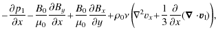
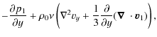
and substituting those expressions into the viscous, non-resistive,
two-dimensional MHD equations, with no gravity force for simplicity,
and neglecting terms involving products of perturbations, we obtain the
following set of linearized equations, in scalar form:
,
and a background plasma of a constant gas pressure, density and
temperature. The initial disturbances are supposed to be small, in
order to stay in the linear regime. Expressing each quantity q(x,y,t) as the sum of a background constant value plus a perturbation,
q(x,y,t)=q0+q1(x,y,t),
and substituting those expressions into the viscous, non-resistive,
two-dimensional MHD equations, with no gravity force for simplicity,
and neglecting terms involving products of perturbations, we obtain the
following set of linearized equations, in scalar form:

where
where
In a general scheme, viscosity would add a heating term to the
energy equation, but this term is second order, and so, the process is
adiabatic within the linear regime, and there is no heating of any kind
taking place. Hence, the entropy per unit mass,
![]() ,
is conserved, for each single fluid element, and for the entire box.
,
is conserved, for each single fluid element, and for the entire box.
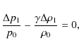
From the conservation of entropy, a relation between the plasma
pressure and density perturbations may be obtained, within first order
(i.e. neglecting the terms involving products of perturbations):
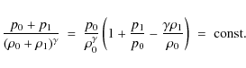
Hence,
where

where
To solve these equations, we first determine the solution for a one-dimensional perturbation, which depends only on x (Sect. 2.1), then only on y (Sect. 2.2), and finally, using the 1D results, we derive the solution for a more general 2D perturbation (Sect. 2.3).
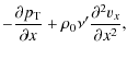
2.1 Perturbation dependent on x
Consider a perturbation varying only in the direction perpendicular to the magnetic field lines, x. The magnetic field vector will have a non-zero y-component,
![]() ,
while the velocity will have a non-zero x-component,
,
while the velocity will have a non-zero x-component,
![]() .
Equations (1) to (6) reduce to
.
Equations (1) to (6) reduce to


with
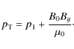
The equation governing the final equilibrium state can be obtained using Eq. (10). At equilibrium, the time dependence disappears, and the velocity is zero, thus, the equilibrium must have constant total pressure:

Combining Eqs. (11) and (12), we get the evolution of the total pressure as
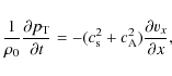
where
Assuming that the total pressure can be considered as a continuous, periodic function, the solution of the last equation can be expressed as a superposition of plane waves, such as
where each wave number k corresponds to a different oscillation mode and is associated with a complex frequency
The dispersion relation has the solution
In order to have a harmonic mode, the wave number k must satisfy
where Lx is the length of the x-domain.
From the solution of Eq. (16), and Eq. (15), we obtain an expression for v1(x,t), which, after substitution into Eqs. (9), (11) and (12), gives
| |
= | 
|
(19) |
| = | 
|
(20) | |
| = | 
|
(21) |
Integrating now from t=0 to
Equations (22)-(24) state that no matter how we set our initial disturbance, the final equilibrium distributions are completely determined by the initial and the final total pressures of the system, which are given by the solution of the wave equation. Note, that also the adiabatic equation for the linear regime given in Eq. (8) is satisfied.
2.2 Perturbation dependent on y
In the same way as above, we can get the solution for a perturbation
varying only along the field. This time, we are dealing with a purely
non-magnetic evolution, that will lead to a homogeneous redistribution
of the plasma pressure all along the field lines. The equations to
solve are the y-components of Eqs. (1), (3) and (4). The equilibrium is now given by

and the solution for the perturbed quantities is
| |
= | (26) | |
| = | (27) |
where Ly is the length of the y-domain.
2.3 Two-dimensional perturbation
In this section, we study the relaxation of a general individual
two-dimensional perturbation within the linear regime. Once again,
setting the velocities to zero, we get the equations governing the
final 2D equilibrium:
Equation (29) tells us that the final plasma pressure cannot depend on y, so the solution for the pressure must remain one-dimensional, as before. On the other hand, Eq. (28) does not have a direct interpretation, as both spatial derivatives are involved. The term
where:
- i.
- The mode
 represents the unperturbed background values.
- ii.
- For
 ,
the equation of the equilibrium is
,
the equation of the equilibrium is
(30)
These modes only depend on x, and represent the homogeneous redistribution of the total pressure studied in Sect. 2.1. - iii.
- For
 we get
 = 0,
= 0,
(31)  = 0.
= 0.
(32)
These modes do not modify By, instead they simply remove both the vertical gradients of magnetic tension and plasma pressure as in Sect. 2.2. Each of them is treated individually, as they are not coupled in the equations. - iv.
- Finally, for those modes with
 ,
we get
kBy - lBx = 0,
,
we get
kBy - lBx = 0,
which can be combined with the solenoidal condition for the magnetic field, ,
or, within our fourier notation,
kBy + lBx = 0.
,
or, within our fourier notation,
kBy + lBx = 0.
From these equations, we can conclude that, in the final equilibrium, the existance of a variation of By in the x-direction is totally incompatible with a variation of Bx in the y-direction. Hence, the modes with both wave numbers k and l non-zero may appear in the dynamical evolution, but not in the final equilibrium distributions.
Hence, we calculate the analytical 2D equilibrium in two steps: Firstly, the non-magnetic evolution in the vertical direction,
and secondly, the hydromagnetic evolution in the horizontal direction, across the field,
In Eqs. (33) to (37) the quantities with a superscript represent the state after the vertical evolution, with
Looking back at the equations, we see a well known result from magnetohydrostatics, namely: In equilibrium, and in the absence of gravity, the plasma pressure must be constant along the field lines. The constant plasma pressure in the y-direction given by Eq. (29) is aligned with the straight magnetic configuration, with no magnetic tension, for the final equilibrium state.
When analyzing the validity of the results above for a non-ideal experiment, it is important to remember that Eqs. (34) to (37) come from the linear approximation, but Eq. (33)
does not. Hence, we expect our analytical calculations for the pressure
to hold for much larger initial perturbations than the ones for the
density. If the initial pressure disturbance is not small, but the
linear expression for the plasma pressure is still valid, the adiabatic
condition (i.e. conservation of entropy), which is more robust than the
linear calculations, gives us a better approximation for the final
equilibrium plasma density, calculated as
3 Numerical experiments
To investigate the validity of the analytical results, we have used
Lare2D, a staggered Lagrangian-remap code with user controlled
viscosity, to solve the full MHD equations, with the resistivity set to
zero (for further details, see Arber et al. 2001). The numerical domain is a square box with a uniform grid of
![]() points. The background magnetic field is pointing in the vertical y-direction and all the perturbations depend on both x and y.
The top and bottom boundaries of the box are periodic, so that the
field lines are not line-tied. The boundaries on the left and right
sides are closed. The choice of either closed or periodic side
boundaries makes no difference for our experiments. There is neither
mass nor energy flowing across the side boundaries.
points. The background magnetic field is pointing in the vertical y-direction and all the perturbations depend on both x and y.
The top and bottom boundaries of the box are periodic, so that the
field lines are not line-tied. The boundaries on the left and right
sides are closed. The choice of either closed or periodic side
boundaries makes no difference for our experiments. There is neither
mass nor energy flowing across the side boundaries.
The numerical code uses the normalised MHD equations, where the normalised magnetic field, density and lengths,
imply that the normalising constants for pressure, internal energy and current density are
We have used here the subscript n for the normalising constants, instead of 0, to avoid confusion with the initial background values. The hat quantities are the dimensionless variables with which the code works. The expression for the plasma beta can be obtained from this normalisation as
|
(39) |
The initial disturbance consists of an internal energy and pressure enhancement, leaving the initial plasma density and magnetic field undisturbed. The perturbation is taken as a single two-dimensional Gaussian centered in the middle of the box:
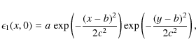
|
(40) |
with b=0.5L and c=0.05L. As there is no initial perturbation of the magnetic field, the initial perturbed total pressure is just the perturbed plasma pressure, and the final analytical perturbed total pressure is the average value of that initial perturbed plasma pressure distribution, so that

For the experiment shown here, we have chosen a rather large perturbation, of the same order as the background value, i.e.
Figure 1 shows the time
evolution of the various energies of the system, integrated over the
whole box. Kinetic energy (in green) grows quickly from zero to its
maximum value, and is subsequently damped to zero in the final
equilibrium. A small fraction of the internal energy is converted into
magnetic energy at the new equilibrium. For this particular set up, in
which the perturbation has been introduced in the plasma pressure, it
is the plasma that loses some of its initial internal energy,
transfering it to the magnetic field. Note, that the amount of energy
transfered is directly proportional to the magnitude of the
perturbation. The total energy (i.e. the sum of the magnetic, kinetic
and internal energies) is conserved to an accuracy of ![]() 10-7.
10-7.
![\begin{figure}
\par\includegraphics[width=9cm,clip]{13902fg1.eps}
\end{figure}](/articles/aa/full_html/2010/06/aa13902-09/img97.png)
|
Figure 1:
Time evolution of the energies for the case where
|
| Open with DEXTER | |
![\begin{figure}
\par\includegraphics[width=9cm,clip]{13902fg2.eps}
\end{figure}](/articles/aa/full_html/2010/06/aa13902-09/img98.png)
|
Figure 2: Two-dimensional contour plots of plasma pressure ( top), plasma density ( center) and current density ( bottom) in the initial state ( left column) and final equilibrium ( right column), for the same experiment as Fig. 1. |
| Open with DEXTER | |
The 2D contour plots of the normalised plasma pressure, density and perpendicular current density for the initial and final equilibrium state are shown in Fig. 2 for this case. The initial increase of plasma pressure creates a localized decrease in plasma density. The displacement of the magnetic field lines is hard to appreciate from the field lines themselves, but is clear from the non-zero perpendicular electric current density, jz, that exists in the final equilibrium.
Figures 3 and 4 show vertical cuts at x=L/2 and horizontal cuts at y=L/2, respectively, through the contour plots in Fig. 2,
for the relevant quantities for the initial and final state. In these
plots, a detailed comparison of the numerical and analytical solutions
can be made. The analytical predictions for total pressure are very
good, even though the amplitude of the perturbation is relatively large
(
![]() )
and so, strictly speaking, our analytical approximation should not
hold. However, the linear approximation for the plasma density (red
crosses in Figs. 3 and 4) does not fit well. Instead, if we use Eq. (38),
a much better fit for the plasma density is found (blue crosses in the
plots), implying that the process is approximately adiabatic. Since the
numerical experiments have been performed using a full MHD code that
solves the non-linear equations, the process is not entirely adiabatic,
but must have a finite amount of viscous heating that will become
important as the initial perturbation is increased.
)
and so, strictly speaking, our analytical approximation should not
hold. However, the linear approximation for the plasma density (red
crosses in Figs. 3 and 4) does not fit well. Instead, if we use Eq. (38),
a much better fit for the plasma density is found (blue crosses in the
plots), implying that the process is approximately adiabatic. Since the
numerical experiments have been performed using a full MHD code that
solves the non-linear equations, the process is not entirely adiabatic,
but must have a finite amount of viscous heating that will become
important as the initial perturbation is increased.
4 Importance of non-linear effects
To study how non-linearity affects the results as the magnitude of the initial perturbation increases, we focus again on the total pressure. The total pressure of the final numerical equilibrium must be constant, whether the relaxation remains in the linear regime or not. On the other hand, the analytical definition of total pressure given by (13) is an approximation from the linear analysis, and will become less valid as the non-linear terms become more important. We perform a series of experiments for various plasma beta values in which the relative amplitude of the initial perturbation is changed from a very small value, well within the linear regime, to a large value way outside it. Using these experiments, we investigate how the final total pressure departs from the linear predictions for different background plasma beta values.
But first, we recall that the 2D relaxation may be separated
into a vertical non-magnetic evolution (vertical redistribution of
plasma pressure) and a horizontal evolution (horizontal redistribution
of total pressure), in which the total pressure in the vertical case is
not
determined by the linear analysis. This suggests that, effectively, in
order to find a significant error in the final total pressure for the
2D experiment, we will need very large values of the initial
two-dimensional perturbation. Hence, the following experiments have
been made for just a one-dimensional perturbation across the field
lines. These results may be mapped onto those for our intital 2D
perturbation, using the following:
Figure 5 shows the relative error of the linear aproximation in both 1D and 2D for the total pressure, as a function of the amplitude of the initial perturbation, for five different values of the plasma beta (
where
with
| Figure 3: Vertical cuts for the plasma pressure (left) and plasma density ( right), for the same experiment as Figs. 1 and 2. Initial perturbed state (dashed) is compared with the final equilibrium, as found by the full MHD numerical simulations (solid) and predicted by the linear analysis (red crosses). For the density predictions, the blue crosses represent predictions from the adiabatic condition given by Eq. (38). |
|
| Open with DEXTER | |
![\begin{figure}
\par\includegraphics[width=9cm,clip]{13902fg4.eps}
\end{figure}](/articles/aa/full_html/2010/06/aa13902-09/img110.png)
|
Figure 4: Horizontal cuts for the plasma pressure (top left), plasma density (top right), total pressure (bottom left) and magnetic field strength (bottom left), for the same experiment as Figs. 1, 2 and 3. |
| Open with DEXTER | |
![\begin{figure}
\par\includegraphics[width=9cm,clip]{13902fg5.eps}
\end{figure}](/articles/aa/full_html/2010/06/aa13902-09/img111.png)
|
Figure 5: Relative error in the linear prediction of the total pressure against the magnitude of the initial pressure perturbation, for five different values of the plasma beta. The slow growth rate of the error (non-linear effects) indicates the validity of the linear analysis studied in this paper. |
| Open with DEXTER | |
As
![]() ,
we expect the relative error of the linear analysis to tend to zero,
independently of the perturbation, as in this case, the magnetic
effects dissapear, and the initial pressure perturbation completely
redistributes to a well defined constant value in the whole box. On the
other hand, if
,
we expect the relative error of the linear analysis to tend to zero,
independently of the perturbation, as in this case, the magnetic
effects dissapear, and the initial pressure perturbation completely
redistributes to a well defined constant value in the whole box. On the
other hand, if
![]() ,
then the magnetic field will dominate over the plasma contributions, and much larger values for the relative initial perturbation will be needed for strictly leaving the linear regime. These two behaviors can be seen in Fig. 5,
where the plots for large plasma-betas tend to a smaller error, while
the plots for small plasma-betas take longer to reach significant
errors, i.e. to escape from the linear regime. Furthermore, we must not
forget that we are here only talking about the initial background
plasma beta, so a large background beta combined with a large initial
perturbation will make the final plasma beta even higher. Thus,
,
then the magnetic field will dominate over the plasma contributions, and much larger values for the relative initial perturbation will be needed for strictly leaving the linear regime. These two behaviors can be seen in Fig. 5,
where the plots for large plasma-betas tend to a smaller error, while
the plots for small plasma-betas take longer to reach significant
errors, i.e. to escape from the linear regime. Furthermore, we must not
forget that we are here only talking about the initial background
plasma beta, so a large background beta combined with a large initial
perturbation will make the final plasma beta even higher. Thus,
![]() will imply
will imply
![]() for the final equilibrium, so we expect the curves of the relative
error of the linear analysis to turn back to zero as the initial
perturbation is greatly increased. In terms of energy conservation, as
the velocity is zero at the initial and final states, the integral over
the whole domain of internal energy plus magnetic energy must be
conserved: if
for the final equilibrium, so we expect the curves of the relative
error of the linear analysis to turn back to zero as the initial
perturbation is greatly increased. In terms of energy conservation, as
the velocity is zero at the initial and final states, the integral over
the whole domain of internal energy plus magnetic energy must be
conserved: if
![]() ,
then the internal energy is much larger than the magnetic energy, and
will just redistribute the plasma pressure, without transferring any
energy into the magnetic field.
,
then the internal energy is much larger than the magnetic energy, and
will just redistribute the plasma pressure, without transferring any
energy into the magnetic field.
On the contrary, the final plasma density is entirely
determined by the linear analysis, in both the vertical and the
horizontal evolutions along and across the field lines, or in a better
approximation, by the adiabatic condition. Hence, the non-linear
effects for the plasma density will grow much quicker, as shown in
Fig. 6. These last numerical experiments have been made for the original two-dimensional Gaussian perturbation. The error on the y-axis is given by
where
The relative error in the plasma density is considerably bigger than
the relative error in pressure, and so, for only a small change in p1/p0 in the 2D case, we find a large error in ![]() .
As this error quickly reaches significant values, the plasma beta plays
much less of a role for the non-linear effects in the plasma density
than in the above total pressure.
.
As this error quickly reaches significant values, the plasma beta plays
much less of a role for the non-linear effects in the plasma density
than in the above total pressure.
![\begin{figure}
\par\includegraphics[width=9cm,clip]{13902fg6.eps}
\end{figure}](/articles/aa/full_html/2010/06/aa13902-09/img118.png)
|
Figure 6: Relative error of the density predicted assuming an adiabatic evolution, with Eq. (38), against the magnitude of the 2D initial pressure perturbation, for three values of the plasma beta. Note, that the x-axis in this plot is to be compared with the top x-axis in Fig. 5. |
| Open with DEXTER | |
5 Summary and conclusions
We have presented analytical and numerical calculations for the 2D magnetohydrodynamic relaxation of an untwisted perturbed magnetic system embedded in a plasma with beta of any size, and find a final equlibrium state which differs substantially from the initial background configuration. The equilibrium reached is a non force-free state in which the plasma pressure gradients are balanced by the magnetic Lorentz force. For a set of specified boundaries, all the hydromagnetic quantities are fully determined by the initial perturbed state.
The initial disturbance evolves into the final relaxed state by different families of magnetoacoustic waves, dissipated via viscous damping. Fast magnetoacoustic waves propagate across the field lines in the horizontal direction, slow magnetoacoustic waves redistribute the thermodynamic quantities along the field in the vertical direction, and an extra contribution of slow magnetoacoustic waves propagates along the magnetic field lines introducing a magnetic tension term. Nevertheless, these last slow magnetoacoustic waves dissipate the magnetic tension in such a way that it is totally unimportant when determining the final equilibrium distributions. The vertical redistribution of the plasma pressure to a homogeneous value demands the magnetic tension to dissapear completely, so both the plasma pressure and total pressure are one-dimensional at the end of the process.
Within the linear regime, the final distributions are completely independent of the viscosity, even though it is required to permit the relaxation to ocurr, as it is the only damping mechanism of the waves. An increase in the viscosity enhances the diffusive term in the wave equation, and so, accelerates the process, but the final distribution is not modified. Instead, in the final equilibrium, all the quantities are simply determined by the behaviour of the final equilibrium total pressure, involving plasma and magnetic effects. Hence, the final equilibrium states for plasma pressure and magnetic field do not differ if the initial perturbation is of the density, temperature or internal energy.
Finally, by investigating the linear regime, we have been able to make analytical predictions for the final MHS equilibrium, even when the regime is far from linear. The linear predictions remain remarkably valid even outside the linear regime, as the growth rate of the non-ideal effects is very small, compared to the initial perturbations.
In this paper, the introduction of plasma effects in the relaxation of hydromagnetic systems have been studied in simple schemes, producing a series of analytical predictions which have been confirmed by our numerical results. By starting with a uniform magnetic field, we have reached a state in which the magnetic field itself remains almost uniform, but where some current density has been built. Also, even in this simple configuration, a non-neglectible amount of energy has been transferred from the plasma to the magnetic field. These implications of energy transfer during the relaxation process indicate that this process will be of importance in the solar corona, specially in the study of magnetic null points and their surroundings. Null points have been found to have a reasonable population density in the Solar Corona by Longcope & Parnell (2009). In further studies, we will consider more complex scenarios, introducing two-dimensional null points and starting to consider the implications of non-zero plasma betas in three-dimensional magnetic environments.
References
- Amari, T., Boulmezaoud, T. Z., & Maday, Y. 1998, A&A, 339, 252 [NASA ADS] [Google Scholar]
- Arber, T. D., Longbottom, A. W., Gerrard, C. L., & Milne, A. M. 2001, Computational Phys., 171, 151 [Google Scholar]
- Browning, P. K., Gerrard, C., Hood, A. W., Kevis, R., & van der Linden, R. A. M. 2008, A&A, 485, 837 [NASA ADS] [CrossRef] [EDP Sciences] [Google Scholar]
- De Rosa, M. L., Schrijver, C. J., Barnes, G., et al. 2009, ApJ, 696, 1780 [Google Scholar]
- Gary, G. A. 2001, Sol. Phys., 203, 71 [NASA ADS] [CrossRef] [Google Scholar]
- Gary, G. A. 2009, Sol. Phys., 257, 271 [NASA ADS] [CrossRef] [Google Scholar]
- Heyvaerts, J., & Priest, E. R. 1984, A&A, 137, 63 [NASA ADS] [Google Scholar]
- Hood, A. W., Browning, P. K., & van der Linden, R. A. M. 2009, A&A, 506, 913 [NASA ADS] [CrossRef] [EDP Sciences] [Google Scholar]
- Inoue, S., Kusano, K., Masuda, S., et al. 2008, in First Results From Hinode, ed. S. A. Matthews, J. M. Davis, & L. K. Harra, ASP Conf. Ser., 397, 110 [Google Scholar]
- Janse, Å. M., & Low, B. C. 2009, ApJ, 690, 1089 [NASA ADS] [CrossRef] [Google Scholar]
- Ji, H., Huang, G., & Wang, H. 2007, ApJ, 660, 893 [NASA ADS] [CrossRef] [Google Scholar]
- Longcope, D. W., & Parnell, C. E. 2009, Sol. Phys., 254, 51 [NASA ADS] [CrossRef] [Google Scholar]
- Low, B. C. 2006, ApJ, 649, 1064 [NASA ADS] [CrossRef] [Google Scholar]
- Mackay, D. H., & van Ballegooijen, A. A. 2006, ApJ, 641, 577 [NASA ADS] [CrossRef] [Google Scholar]
- McLaughlin, J. A., & Hood, A. W. 2006, A&A, 459, 641 [NASA ADS] [CrossRef] [EDP Sciences] [Google Scholar]
- Metcalf, T. R., De Rosa, M. L., Schrijver, C. J., et al. 2008, Sol. Phys., 247, 269 [Google Scholar]
- Miller, K., Fornberg, B., Flyer, N., & Low, B. C. 2009, ApJ, 690, 720 [NASA ADS] [CrossRef] [Google Scholar]
- Pontin, D. I., Hornig, G., Wilmot-Smith, A. L., & Craig, I. J. D. 2009, ApJ, 700, 1449 [NASA ADS] [CrossRef] [Google Scholar]
- Priest, E. R. 1982, Solar magneto-hydrodynamics, 74 [Google Scholar]
- Régnier, S. 2008, in First Results From Hinode, ed. S. A. Matthews, J. M. Davis, & L. K. Harra, ASP Conf. Ser., 397, 75 [Google Scholar]
- Ruan, P., Wiegelmann, T., Inhester, B., et al. 2008, A&A, 481, 827 [NASA ADS] [CrossRef] [EDP Sciences] [Google Scholar]
- Schrijver, C. J., De Rosa, M. L., Metcalf, T. R., et al. 2006, Sol. Phys., 235, 161 [Google Scholar]
- Schrijver, C. J., De Rosa, M. L., Metcalf, T., et al. 2008, ApJ, 675, 1637 [Google Scholar]
- Taylor, J. B. 1974, Phys. Rev. Lett., 33, 1139 [NASA ADS] [CrossRef] [Google Scholar]
- Wheatland, M. S., & Régnier, S. 2009, ApJ, 700, L88 [NASA ADS] [CrossRef] [Google Scholar]
- Wiegelmann, T., Inhester, B., & Sakurai, T. 2006, Sol. Phys., 233, 215 [NASA ADS] [CrossRef] [Google Scholar]
- Wiegelmann, T., Thalmann, J. K., Schrijver, C. J., De Rosa, M. L., & Metcalf, T. R. 2008, Sol. Phys., 247, 249 [NASA ADS] [CrossRef] [Google Scholar]
All Figures
|
|
Figure 1:
Time evolution of the energies for the case where
|
| Open with DEXTER | |
| In the text | |
|
|
Figure 2: Two-dimensional contour plots of plasma pressure ( top), plasma density ( center) and current density ( bottom) in the initial state ( left column) and final equilibrium ( right column), for the same experiment as Fig. 1. |
| Open with DEXTER | |
| In the text | |
| |
Figure 3: Vertical cuts for the plasma pressure (left) and plasma density ( right), for the same experiment as Figs. 1 and 2. Initial perturbed state (dashed) is compared with the final equilibrium, as found by the full MHD numerical simulations (solid) and predicted by the linear analysis (red crosses). For the density predictions, the blue crosses represent predictions from the adiabatic condition given by Eq. (38). |
| Open with DEXTER | |
| In the text | |
|
|
Figure 4: Horizontal cuts for the plasma pressure (top left), plasma density (top right), total pressure (bottom left) and magnetic field strength (bottom left), for the same experiment as Figs. 1, 2 and 3. |
| Open with DEXTER | |
| In the text | |
|
|
Figure 5: Relative error in the linear prediction of the total pressure against the magnitude of the initial pressure perturbation, for five different values of the plasma beta. The slow growth rate of the error (non-linear effects) indicates the validity of the linear analysis studied in this paper. |
| Open with DEXTER | |
| In the text | |
|
|
Figure 6: Relative error of the density predicted assuming an adiabatic evolution, with Eq. (38), against the magnitude of the 2D initial pressure perturbation, for three values of the plasma beta. Note, that the x-axis in this plot is to be compared with the top x-axis in Fig. 5. |
| Open with DEXTER | |
| In the text | |
Copyright ESO 2010
Current usage metrics show cumulative count of Article Views (full-text article views including HTML views, PDF and ePub downloads, according to the available data) and Abstracts Views on Vision4Press platform.
Data correspond to usage on the plateform after 2015. The current usage metrics is available 48-96 hours after online publication and is updated daily on week days.
Initial download of the metrics may take a while.