| Issue |
A&A
Volume 514, May 2010
|
|
|---|---|---|
| Article Number | A62 | |
| Number of page(s) | 14 | |
| Section | Stellar structure and evolution | |
| DOI | https://doi.org/10.1051/0004-6361/200913684 | |
| Published online | 20 May 2010 | |
Effects of the variation of fundamental constants on Population III stellar evolution
S. Ekström1 - A. Coc2 - P. Descouvemont3 - G. Meynet1 - K. A. Olive4 - J.-P. Uzan5,6 - E. Vangioni5
1 - Geneva Observatory, University of Geneva, Maillettes 51, 1290
Sauverny, Switzerland
2 - Centre de Spectrométrie Nucléaire et de Spectrométrie de Masse
(CSNSM), UMR 8609, CNRS/IN2P3 and Université Paris Sud 11,
Bâtiment 104, 91405 Orsay Campus, France
3 - Physique Nucléaire Théorique et Physique Mathématique, CP 229,
Université Libre de Bruxelles (ULB), 1050 Brussels, Belgium
4 - William I. Fine Theoretical Physics Institute, University of
Minnesota, Minneapolis, Minnesota 55455, USA
5 - Institut d'Astrophysique de Paris, UMR-7095 du CNRS, Université
Pierre et Marie Curie, 98 bis bd Arago, 75014 Paris, France
6 - Department of Mathematics and Applied Mathematics, University of
Cape Town, Rondebosch 7701, Cape Town, South Africa
Received 17 November 2009 / Accepted 1 February 2010
Abstract
Aims. A variation of the fundamental constants is
expected to affect the thermonuclear rates important for stellar
nucleosynthesis. In particular, because of the very low
resonant energies of 8Be and 12C,
the triple ![]() process is extremely sensitive to any such variations.
process is extremely sensitive to any such variations.
Methods. Using a microscopic model for these nuclei,
we derive the sensitivity of the Hoyle state to the nucleon-nucleon
potential, thereby allowing for a change in the magnitude of the
nuclear interaction. We follow the evolution of 15 and 60 ![]() zero-metallicity stellar models, up to the end of core helium
burning. These stars are assumed to be representative of the first,
Population III stars.
zero-metallicity stellar models, up to the end of core helium
burning. These stars are assumed to be representative of the first,
Population III stars.
Results. We derive limits on the variation in the
magnitude of the nuclear interaction and model dependent limits on the
variation of the fine structure constant based on the calculated oxygen
and carbon abundances resulting from helium burning. The requirement
that some 12C and 16O
be present at the end of the helium burning phase allows for permille
limits on the change in the nuclear interaction and limits of the order
of 10-5 on the fine structure constant
relevant at a cosmological redshift of
![]() .
.
Key words: atomic processes - nuclear reactions, nucleosynthesis, abundances - stars: chemically peculiar - stars: evolution - early Universe - cosmological parameters
1 Introduction
The equivalence principle is a cornerstone of metric theories of
gravitation and in particular of general relativity (Will 1993). This principle,
including the universality of free fall, the local position and Lorentz
invariances, postulates that the local laws of physics and,
in particular the values of the dimensionless constants such
as the fine structure constant
![]() ,
must remain fixed and thus be the same at any time and in any place.
It follows that by testing the constancy of fundamental
constants one actually performs a test of General Relativity, which can
be extended on astrophysical and cosmological scales (for a review, see
Uzan 2003,2009a)
,
must remain fixed and thus be the same at any time and in any place.
It follows that by testing the constancy of fundamental
constants one actually performs a test of General Relativity, which can
be extended on astrophysical and cosmological scales (for a review, see
Uzan 2003,2009a)
We define a fundamental constant as any free parameter of the fundamental theories at hand (Duff 2002; Duff et al. 2002; Barrow 2002; Uzan & Leclercq 2008; Weinberg 1983). These parameters are contingent quantities that can only be measured and are assumed constant since (i) in the theoretical framework in which they appear, there is no equation of motion for them and they cannot be deduced from other constants; and (ii) if the theories in which they appear have been validated experimentally, it means that these parameters have indeed been checked to be constant at the precision of the experiments. By testing for their constancy we extend our knowledge of the domain of validity of the theories in which they appear. In that respect, astrophysics and cosmology allow one to probe the largest time-scales, typically close to the age of the universe.
One can, however, question the constancy of these
dimensionless numbers and the physics that determine their value. This
sends us back to the phenomenological argument by Dirac (1937), known as the ``large
number hypothesis'', according to which the dimensionless ratio
![]() ,
or simply G in atomic units, should
decrease as the inverse of the age of the universe, followed
by Jordan (1937),
who formulated a field theory in which both the fine structure constant
and the gravitational constant were replaced by dynamical fields. It
was soon pointed out by Fierz
(1956) that astronomical observations can set strong
constraints on the variations of these constants. This paved the way to
two complementary directions in the research on the fundamental
constants.
,
or simply G in atomic units, should
decrease as the inverse of the age of the universe, followed
by Jordan (1937),
who formulated a field theory in which both the fine structure constant
and the gravitational constant were replaced by dynamical fields. It
was soon pointed out by Fierz
(1956) that astronomical observations can set strong
constraints on the variations of these constants. This paved the way to
two complementary directions in the research on the fundamental
constants.
On the one hand, from a theoretical perspective, many theories involving ``varying constants'' have been designed. This is in particular the case of theories involving extra dimensions, such as the Kaluza-Klein mechanism (Kaluza 1921; Klein 1926) and string theory, in which all the constants (including gauge, Yukawa and gravitational couplings) are dynamical quantities (Wetterich 1988; Taylor & Veneziano 1988; Witten 1984; Wu & Wang 1986), or in theories such as scalar-tensor theories of gravity (Jordan 1949; Brans & Dicke 1961; Damour & Esposito-Farese 1992) and in many models of quintessence (Damour et al. 2002a,b; Lee et al. 2004; Uzan 1999; Wetterich 2003; Riazuelo & Uzan 2002) that aim at explaining the acceleration of the universe by the dynamics of a scalar field. It is impingent on these models to explain why the constants are so constant today and provide a mechanism for fixing their value (Damour & Polyakov 1994; Damour & Nordtvedt 1993). In this respect, testing for the constancy of the fundamental constants is one of the few windows on these theories.
On the other hand, from an experimental and observational
perspective, the variations of various constants have been severely
constrained. This is the case for the fine structure constant for which
the constraint
![]()
![]()
![]() at
z=0 has been obtained from comparing aluminium
and mercury single-ion optical clocks (Rosenband
et al. 2008). On a longer timescale, it was
demonstrated that
at
z=0 has been obtained from comparing aluminium
and mercury single-ion optical clocks (Rosenband
et al. 2008). On a longer timescale, it was
demonstrated that
![]() cannot have varied by more
than 10-7
over the last 2 Gyr from the Oklo phenomenon (Olive et al.
2002; Fujii
et al. 2000; Shlyakhter 1976; Damour &
Dyson 1996; Petrov
et al. 2006; Flambaum & Wiringa 2009) and
over the last 4.5 Gyr from meteorite dating (Dyson 1972;
Dicke 1959;
Olive
et al. 2004; Fujii & Iwamoto 2003).
At higher redshift,
0.4 < z < 3.5, there are conflicting
reports of an observed variation of
cannot have varied by more
than 10-7
over the last 2 Gyr from the Oklo phenomenon (Olive et al.
2002; Fujii
et al. 2000; Shlyakhter 1976; Damour &
Dyson 1996; Petrov
et al. 2006; Flambaum & Wiringa 2009) and
over the last 4.5 Gyr from meteorite dating (Dyson 1972;
Dicke 1959;
Olive
et al. 2004; Fujii & Iwamoto 2003).
At higher redshift,
0.4 < z < 3.5, there are conflicting
reports of an observed variation of
![]() from quasar absorption
systems. Using the many-multiplet method, Webb
et al. (2001) and Murphy
et al. (2003,2007) claim a statistically
significant variation
from quasar absorption
systems. Using the many-multiplet method, Webb
et al. (2001) and Murphy
et al. (2003,2007) claim a statistically
significant variation
![]()
![]() 10-5, indicating a smaller value of
10-5, indicating a smaller value of
![]() in the past. More recent
observations taken at VLT/UVES using the many
multiplet method have not been able to duplicate the previous result (Quast
et al. 2004; Srianand et al. 2004,2007;
Chand
et al. 2004). The use of Fe lines in Quast et al. (2004) on a
single absorber found
in the past. More recent
observations taken at VLT/UVES using the many
multiplet method have not been able to duplicate the previous result (Quast
et al. 2004; Srianand et al. 2004,2007;
Chand
et al. 2004). The use of Fe lines in Quast et al. (2004) on a
single absorber found
![]()
![]() 10-5. However, since the previous result relied
on a statistical average of over 100 absorbers, it is
not clear that these two results are in contradiction. In Chand et al. (2004), the
use of Mg and Fe lines in a set of 23 systems yielded
the result
10-5. However, since the previous result relied
on a statistical average of over 100 absorbers, it is
not clear that these two results are in contradiction. In Chand et al. (2004), the
use of Mg and Fe lines in a set of 23 systems yielded
the result
![]()
![]() 10-5 and therefore represents a more significant
disagreement and can be used to set very stringent limits on the
possible variation of
10-5 and therefore represents a more significant
disagreement and can be used to set very stringent limits on the
possible variation of
![]() .
A purely astrophysical explanation for these results is also
possible (Ashenfelter
et al. 2004a,b). At larger redshifts, constraints
at the percent level have been obtained from the observation of the
temperature anisotropies of cosmic microwave background at (
.
A purely astrophysical explanation for these results is also
possible (Ashenfelter
et al. 2004a,b). At larger redshifts, constraints
at the percent level have been obtained from the observation of the
temperature anisotropies of cosmic microwave background at (
![]() )
(e.g. Martins
et al. 2004; Nakashima et al. 2008; Stefanescu 2007;
Scóccola
et al. 2008) and from big bang nucleosynthesis (BBN)
(
)
(e.g. Martins
et al. 2004; Nakashima et al. 2008; Stefanescu 2007;
Scóccola
et al. 2008) and from big bang nucleosynthesis (BBN)
(
![]() )
(e.g. Müller
et al. 2004; Flambaum & Shuryak 2002; Dent et al.
2007; Bergström
et al. 1999; Campbell & Olive 1995;
Kolb
et al. 1986; Nollett & Lopez 2002; Landau et al.
2006; Coc
et al. 2007; Ichikawa & Kawasaki 2004,2002).
We refer to Uzan
(2004,2003,2009b)
for recent reviews on this topic. For the time being, there is no
constraint on
)
(e.g. Müller
et al. 2004; Flambaum & Shuryak 2002; Dent et al.
2007; Bergström
et al. 1999; Campbell & Olive 1995;
Kolb
et al. 1986; Nollett & Lopez 2002; Landau et al.
2006; Coc
et al. 2007; Ichikawa & Kawasaki 2004,2002).
We refer to Uzan
(2004,2003,2009b)
for recent reviews on this topic. For the time being, there is no
constraint on
![]() for redshifts ranging
from 4 to 103
although it has been proposed that 21 cm observations may
allow one to fill in the range 30<z<100
(Khatri & Wandelt 2007).
for redshifts ranging
from 4 to 103
although it has been proposed that 21 cm observations may
allow one to fill in the range 30<z<100
(Khatri & Wandelt 2007).
This article focuses on the effect of the possible variation of the fundamental constants on the stellar evolution of early stars, hence possibly providing constraints in a domain of redshifts where no such constraint is available. A similar issue was actually considered by Gamow (1967) (see also the recent work by Adams 2008) who showed that the evolution of the Sun was able to exclude the Dirac model of a varying gravitational constant. In this case, non-gravitational physics is kept unchanged and the evolution of the star is affected only by the modification of gravity. Changing the non-gravitational sector has more drastic implications on stellar physics since the nuclear physics and thus the cross-sections and reaction rates of all the processes should be modified.
Rozental' (1988)
argued that the synthesis of complex elements in stars (mainly the
possibility of the triple ![]() reaction
(
reaction
(![]() )
as the origin of the production of
)
as the origin of the production of
![]() )
sets constraints on the values of the fine structure and strong
coupling constants. There have been several studies on the sensitivity
of carbon production to the underlying nuclear rates (Schlattl
et al. 2004; Csótó et al. 2001; Tur et al. 2007;
Oberhummer
et al. 2000; Barrow 1987; Fairbairn 1999;
Livio
et al. 1989; Oberhummer et al. 2003).
The production of
)
sets constraints on the values of the fine structure and strong
coupling constants. There have been several studies on the sensitivity
of carbon production to the underlying nuclear rates (Schlattl
et al. 2004; Csótó et al. 2001; Tur et al. 2007;
Oberhummer
et al. 2000; Barrow 1987; Fairbairn 1999;
Livio
et al. 1989; Oberhummer et al. 2003).
The production of
![]() in stars requires a triple
tuning: (i) the decay lifetime
of
in stars requires a triple
tuning: (i) the decay lifetime
of
![]() ,
of order 10-16 s,
is four orders of magnitude longer than the time for two
,
of order 10-16 s,
is four orders of magnitude longer than the time for two ![]() particles
to scatter; (ii) an excited state of the carbon lies just
above the energy of
particles
to scatter; (ii) an excited state of the carbon lies just
above the energy of
![]() and finally (iii) the
energy level of
and finally (iii) the
energy level of
![]() at 7.1197 MeV is non
resonant and below the energy
of
at 7.1197 MeV is non
resonant and below the energy
of
![]() ,
at 7.1616 MeV, which ensures that most of the carbon
synthesised is not destroyed by the capture of an
,
at 7.1616 MeV, which ensures that most of the carbon
synthesised is not destroyed by the capture of an ![]() -particle.
The existence of this excited state of 12C
was actually predicted by Hoyle (1954)
and then observed at the predicted energy by Dunbar
et al. (1953) as well as its decay (Cook et al. 1957). The
variation of any constant which would modify the energy of this
resonance, known as the Hoyle level, would dramatically affect
the production of carbon.
-particle.
The existence of this excited state of 12C
was actually predicted by Hoyle (1954)
and then observed at the predicted energy by Dunbar
et al. (1953) as well as its decay (Cook et al. 1957). The
variation of any constant which would modify the energy of this
resonance, known as the Hoyle level, would dramatically affect
the production of carbon.
Qualitatively, and perhaps counter-intuitively, if the energy
level of the Hoyle level were increased, 12C would
probably be rapidly processed to 16O
since the star would, in fact, need to be hotter for the ![]() reaction
to be triggered. On the other hand, if it is decreased very little
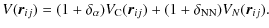
oxygen will be produced. From the general expression of the reaction
rate (see Appendix B
for details, definitions of all the quantities entering this
expression, and a more accurate computation)
reaction
to be triggered. On the other hand, if it is decreased very little
oxygen will be produced. From the general expression of the reaction
rate (see Appendix B
for details, definitions of all the quantities entering this
expression, and a more accurate computation)
![\begin{eqnarray*}\lambda_{3\alpha}=3^{3/2}N_\alpha^3 \left(\frac{2\pi\hbar^3}{M_...
...ar} \exp\left[-\frac{Q_{\alpha\alpha\alpha}}{k_{\rm B}T}\right],
\end{eqnarray*}](/articles/aa/full_html/2010/06/aa13684-09/img33.png)
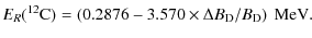
where
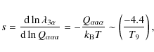
where T9 = T/109 K. This effect was investigated by Csótó et al. (2001) and Oberhummer et al. (2003,2000) who related the variation in
Indeed, modifying the energy of the resonance alone is not realistic since all cross-sections, reaction rates and binding energies etc. should be affected by the variation of the constants. One could indeed have started by assuming independent variations in all these quantities but it is more realistic (and hence more model-dependent) to try to deduce their variation from a microscopic model. Our analysis can then be outlined in three main steps:
- 1.
- Relating the nuclear parameters to fundamental constants such as the Yukawa and gauge couplings, and the Higgs vacuum expectation value. This is a difficult step because of the intricate structure of QCD and its role in low energy nuclear reactions, as in the case of BBN. The nuclear parameters include the set of relevant energy levels (including the ground states), binding energies of each nucleus and the partial width of each nuclear reaction. This involves a nuclear physics model of the relevant nuclei (mainly 4He, 8Be, 12C, and 16O for our study).
- 2.
- Relating the reaction rates to the nuclear parameters, which implies an integration over energy of the cross-sections.
- 3.
- Deducing the change in the stellar evolution (lifetime of the star, abundance of the nuclei, Hertzprung-Russel (HR) diagram, etc.). This involves a stellar model.
The first step is probably the most
difficult. We shall adopt a phenomenological description of the
different nuclei based on a cluster model in which the wave functions
of the 8Be and 12C nuclei
are approximated by a cluster of respectively two and three ![]() wave functions. When solving the associated
Schrödinger equation, we will modify the strength of the
electromagnetic and nuclear N-N interaction potentials
respectively by a factor
wave functions. When solving the associated
Schrödinger equation, we will modify the strength of the
electromagnetic and nuclear N-N interaction potentials
respectively by a factor
![]() and
and
![]() where
where
![]() and
and
![]() are two small dimensionless
parameters that encode the variation of the
fine structure constant and other fundamental couplings. At this stage,
the relation between
are two small dimensionless
parameters that encode the variation of the
fine structure constant and other fundamental couplings. At this stage,
the relation between
![]() and the gauge and Yukawa
couplings is not known. This will allow us to
obtain the energy levels, including the binding energy, of 2H,
4He, 8Be, 12C
and the first
and the gauge and Yukawa
couplings is not known. This will allow us to
obtain the energy levels, including the binding energy, of 2H,
4He, 8Be, 12C
and the first ![]() = 0+ 12C
excited energy level. Note that all of the relevant nuclear states are
assumed to be interacting alpha clusters. In a first
approximation, the variation in the
= 0+ 12C
excited energy level. Note that all of the relevant nuclear states are
assumed to be interacting alpha clusters. In a first
approximation, the variation in the ![]() particle mass
cancels out. The partial widths (and lifetimes) of these states are
scaled from their experimental laboratory values, according to their
energy dependence.
particle mass
cancels out. The partial widths (and lifetimes) of these states are
scaled from their experimental laboratory values, according to their
energy dependence. ![]() is
used as a free parameter. The dependence of the deuterium binding
energy on
is
used as a free parameter. The dependence of the deuterium binding
energy on
![]() then offers us the possibility
of relating this parameter to the gauge
and Yukawa couplings if one matches this prediction to a potential
model via the
then offers us the possibility
of relating this parameter to the gauge
and Yukawa couplings if one matches this prediction to a potential
model via the ![]() and
and ![]() meson
masses (Flambaum
& Shuryak 2003; Damour & Donoghue 2008; Coc et al.
2007; Dmitriev
et al. 2004) or the pion mass, as suggested
by Yoo &
Scherrer (2003); Beane
& Savage (2003); Epelbaum et al. (2003).
meson
masses (Flambaum
& Shuryak 2003; Damour & Donoghue 2008; Coc et al.
2007; Dmitriev
et al. 2004) or the pion mass, as suggested
by Yoo &
Scherrer (2003); Beane
& Savage (2003); Epelbaum et al. (2003).
The second step requires an integration
over energy to deduce the reaction rates as functions of the
temperature and of the new parameters
![]() and
and
![]() .
.
The third step involves stellar models and
in particular some choices about the masses and initial metallicity of
the stars. In a hierarchical scenario of structure formation,
Population III stars (Pop III) were formed
a few ![]() years
after the big bang, that is at a redshift of
years
after the big bang, that is at a redshift of
![]() with zero metallicity. While theoretically uncertain, it is
usually thought that the first stars were massive; however, their mass
range is presently unknown, (for a review, see Bromm et al. 2009).
Pop III stars are interesting to the present study
because of their redshift of formation (as mentioned above)
but also because they are sensitive to the
with zero metallicity. While theoretically uncertain, it is
usually thought that the first stars were massive; however, their mass
range is presently unknown, (for a review, see Bromm et al. 2009).
Pop III stars are interesting to the present study
because of their redshift of formation (as mentioned above)
but also because they are sensitive to the ![]() reaction as early as
Main Sequence (MS): having no initial 12C
to ignite the CNO cycle, they must contract until the
reaction as early as
Main Sequence (MS): having no initial 12C
to ignite the CNO cycle, they must contract until the ![]() reaction
is triggered and some He is burned. We thus focus on Pop III
stars with masses 15 and 60
reaction
is triggered and some He is burned. We thus focus on Pop III
stars with masses 15 and 60 ![]() ,
assuming no rotation. Our computation is stopped at the end of core
helium burning.
,
assuming no rotation. Our computation is stopped at the end of core
helium burning.
The final step uses these predictions to set constraints on the fundamental constants, using stellar constraints such the C/O ratio which is in fact observable in very metal poor stars. While this article can be seen as a theoretical investigation that describes the expected effect of a variation of the fundamental constants, it also sheds some interesting light on stellar physics and its sensitivity to fundamental physics.
The article is logically organised as follows.
Section 2 recalls the basis of the ![]() -reaction, Sect. 3
describes the nuclear physics modelling (first step), Sect. 4
is devoted to stellar implications and Sect. 5 to the
discussion. Technical details are gathered in the Appendices.
-reaction, Sect. 3
describes the nuclear physics modelling (first step), Sect. 4
is devoted to stellar implications and Sect. 5 to the
discussion. Technical details are gathered in the Appendices.
2 Stellar carbon production
TheConsequently, the C and O abundances at the end of helium
burning is very sensitive to small variations in the ![]() reaction
rate. In this context, any anomalous abundance of C
and O in very metal poor stars could potentially be taken as
an indication of the variation in the nucleon - nucleon interaction and
therefore in either or both of the electromagnetic and strong coupling
constants.
reaction
rate. In this context, any anomalous abundance of C
and O in very metal poor stars could potentially be taken as
an indication of the variation in the nucleon - nucleon interaction and
therefore in either or both of the electromagnetic and strong coupling
constants.
![\begin{figure}
\par\includegraphics[width=8cm,clip]{13684fig01.eps}
\vspace*{2.5mm}\end{figure}](/articles/aa/full_html/2010/06/aa13684-09/img46.png)
|
Figure 1:
Level scheme showing the key levels in the |
| Open with DEXTER | |
In our analysis, we focus on the C/O ratio. It is of interest,
therefore, to comment on the destruction of carbon (production
of oxygen) as well as the destruction of oxygen. If the
reaction following the ![]() process,
namely 12C(
process,
namely 12C(![]() ,
, ![]() )16O,
is sufficiently fast, then most
)16O,
is sufficiently fast, then most ![]() particles would be
converted to 16O or heavier nuclei with
little 12C left at the end of helium
burning. However, the fact that in general the
C/O ratio in the Universe is about 0.4 suggests that
the 12C(
particles would be
converted to 16O or heavier nuclei with
little 12C left at the end of helium
burning. However, the fact that in general the
C/O ratio in the Universe is about 0.4 suggests that
the 12C(![]() ,
, ![]() )16O reaction
is sufficiently slow that some 12C remains
after helium exhaustion. The presence of comparable quantities
of C and O implies also that the subsequent 16O(
)16O reaction
is sufficiently slow that some 12C remains
after helium exhaustion. The presence of comparable quantities
of C and O implies also that the subsequent 16O(
![]() ,
, ![]() )20Ne reaction
is not too fast, otherwise O would be converted to Ne
or heavier nuclei and little O would survive during helium
burning. We would like to stress the importance of the nuclear balance
between C and O. The observation of C/O in
very metal poor stars may hold the key to any variation in the chain of
processes described above.
)20Ne reaction
is not too fast, otherwise O would be converted to Ne
or heavier nuclei and little O would survive during helium
burning. We would like to stress the importance of the nuclear balance
between C and O. The observation of C/O in
very metal poor stars may hold the key to any variation in the chain of
processes described above.
In Fig. 1,
we show the low energy level schemes of the nuclei participating to the
4He(
![]() )12C reaction:
4He, 8Be and 12C.
The
)12C reaction:
4He, 8Be and 12C.
The ![]() process
begins when two alpha particles fuse to produce a 8Be nucleus
whose lifetime is only
process
begins when two alpha particles fuse to produce a 8Be nucleus
whose lifetime is only ![]() s
but is sufficiently long so as to allow a second alpha capture into the
second excited level of 12C,
at 7.65 MeV above the ground state (of 12C).
In the following, we shall refer to the successive
s
but is sufficiently long so as to allow a second alpha capture into the
second excited level of 12C,
at 7.65 MeV above the ground state (of 12C).
In the following, we shall refer to the successive ![]() captures
as first and second steps, that is
captures
as first and second steps, that is
![]() Be
Be ![]() and 8Be
and 8Be
![]() C
C
![]() C
C ![]() .
The excited state of 12C corresponds to an
.
The excited state of 12C corresponds to an ![]() = 0 resonance,
as postulated by Hoyle (1954)
in order to increase the cross section during the helium burning phase.
This level decays to the first excited level of 12C
at 4.44 MeV through an E2
(i.e. electric with
= 0 resonance,
as postulated by Hoyle (1954)
in order to increase the cross section during the helium burning phase.
This level decays to the first excited level of 12C
at 4.44 MeV through an E2
(i.e. electric with ![]() = 2 multipolarity)
radiative transition as the transition to the ground state (
= 2 multipolarity)
radiative transition as the transition to the ground state (
![]() )
is suppressed (pair emission only). At temperatures above
)
is suppressed (pair emission only). At temperatures above
![]() ,
which are not relevant for our analysis and therefore not treated, one
should also consider other possible levels above the
,
which are not relevant for our analysis and therefore not treated, one
should also consider other possible levels above the ![]() threshold.
threshold.
We define the following energies:
- ER(8Be)
as the energy of the 8Be ground state with
respect to the
 threshold;
- ER(12C)
as the energy of the Hoyle level with respect to the 8Be +
 threshold, i.e. ER(12C)
  12C(02+) +
 C)
where 12C(02+)
is the excitation energy and
C)
is the particle
separation energy;
C)
where 12C(02+)
is the excitation energy and
C)
is the particle
separation energy;
-
 as
the energy of the Hoyle level with respect to the
as
the energy of the Hoyle level with respect to the  threshold
so that
threshold
so that
-
 (8Be)
as the partial width of the beryllium decay (
(8Be)
as the partial width of the beryllium decay (
 Be
Be  );
);
-
 (12C)
as the partial widths of 8Be
(12C)
as the partial widths of 8Be
 C
C
 C .
C .
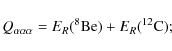
Table 1:
Nuclear data for the two steps of the ![]() -reaction.
-reaction.
Assuming i) thermal equilibrium between the 4He
and 8Be nuclei, so that their
abundances are related by the Saha equation and ii) the sharp
resonance approximation for the alpha capture on 8Be,
the 4He(
![]() )12C rate
can be expressed (Iliadis
2007; Nomoto
et al. 1985) as:
)12C rate
can be expressed (Iliadis
2007; Nomoto
et al. 1985) as:
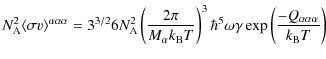
with
During helium burning, the only other important reaction is 12C
![]() O
(Iliadis 2007) which transforms 12C
into 16O. Its competition with the
O
(Iliadis 2007) which transforms 12C
into 16O. Its competition with the ![]() reaction
governs the 12C/16O abundance
ratio at the end of the helium burning phase. Even though, the precise
value of the 12C
reaction
governs the 12C/16O abundance
ratio at the end of the helium burning phase. Even though, the precise
value of the 12C
![]() O
O
![]() -factor
-factor![]() is still a matter
of debate as it relies on an extrapolation of experimental data down to
the astrophysical energy (
is still a matter
of debate as it relies on an extrapolation of experimental data down to
the astrophysical energy (![]() 300 keV),
its energy dependence is much weaker than that of the
300 keV),
its energy dependence is much weaker than that of the ![]() reaction.
Indeed, as it is dominated by broad
resonances, a shift of a few hundred keV in energy
results in a
reaction.
Indeed, as it is dominated by broad
resonances, a shift of a few hundred keV in energy
results in a ![]() -factor
variation of much less than an order of magnitude. For this
reason, we can safely neglect the effect of the 12C
-factor
variation of much less than an order of magnitude. For this
reason, we can safely neglect the effect of the 12C
![]() O reaction
rate variation when compared to the variation in the
O reaction
rate variation when compared to the variation in the ![]() rate.
Similar considerations apply to the rate for 16O
rate.
Similar considerations apply to the rate for 16O
![]() Ne.
Ne.
During hydrogen burning, the pace of the CNO cycle is
given by the slowest reaction, 14N(p,
![]() O. Its
O. Its ![]() -factor
exhibits a well known resonance at 260 keV which is normally
outside of the Gamow energy window (
-factor
exhibits a well known resonance at 260 keV which is normally
outside of the Gamow energy window (![]() 100 keV) but a
variation in the N-N potential could shift its position downward,
resulting in a higher reaction rate and more efficient
CNO H-burning.
100 keV) but a
variation in the N-N potential could shift its position downward,
resulting in a higher reaction rate and more efficient
CNO H-burning.
3 Microscopic determination of the
rate
3.1 Description of the cluster model
In order to analyse the sensitivity of the ![]() reaction to a variation in the strength of the electromagnetic and NN
interactions, we use a microscopic model (see Korennov & Descouvemont 2004;
Wildermuth
& Tang 1977, and references therein). In such an
approach, the wave function of a nucleus with atomic number A,
spin J, and total parity
reaction to a variation in the strength of the electromagnetic and NN
interactions, we use a microscopic model (see Korennov & Descouvemont 2004;
Wildermuth
& Tang 1977, and references therein). In such an
approach, the wave function of a nucleus with atomic number A,
spin J, and total parity ![]() is a solution of a Schrödinger equation with a Hamiltonian given by
is a solution of a Schrödinger equation with a Hamiltonian given by
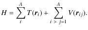
where the potential
The total wave function
When A>4, no exact solutions of
Eq. (5)
can be found and approximate solutions have to be constructed.
For those cases, we use a cluster approximation in
which
![]() is written in terms of
is written in terms of ![]() -nucleus
wave functions. Because the binding energy of the
-nucleus
wave functions. Because the binding energy of the ![]() particle
is large, this approach has been shown to be well adapted to
cluster states, and in particular to 8Be and 12C
(Suzuki
et al. 2008; Kamimura 1981). In the particular
case of these two nuclei, the wave functions are respectively
expressed as
particle
is large, this approach has been shown to be well adapted to
cluster states, and in particular to 8Be and 12C
(Suzuki
et al. 2008; Kamimura 1981). In the particular
case of these two nuclei, the wave functions are respectively
expressed as
where
One then needs to specify the nucleon-nucleon
potential
![]() .
We shall use the microscopic interaction model (Thompson
et al. 1977) which contains one linear parameter
(admixture parameter u), whose standard
value is u=1. It can be slightly modified
to reproduce important inputs, such as the resonance energy of
the Hoyle state. The binding energies of the deuteron
(-2.22 MeV) and of the
.
We shall use the microscopic interaction model (Thompson
et al. 1977) which contains one linear parameter
(admixture parameter u), whose standard
value is u=1. It can be slightly modified
to reproduce important inputs, such as the resonance energy of
the Hoyle state. The binding energies of the deuteron
(-2.22 MeV) and of the ![]() particle
(-24.28 MeV) do not depend on u.
For the deuteron, the Schrödinger equation is solved exactly. More
details about the model are given in Appendix A.
particle
(-24.28 MeV) do not depend on u.
For the deuteron, the Schrödinger equation is solved exactly. More
details about the model are given in Appendix A.
To take into account the variation of the fundamental
constants, we introduce the parameters
![]() and
and
![]() to characterise the change of
the strength of the electromagnetic and
nucleon-nucleon interaction respectively. This is implemented by
modifying the interaction potential (4) so that
to characterise the change of
the strength of the electromagnetic and
nucleon-nucleon interaction respectively. This is implemented by
modifying the interaction potential (4) so that
Such a modification will affect
![\begin{figure}
\par\includegraphics[width=8.8cm,clip]{13684fig02.eps}
\end{figure}](/articles/aa/full_html/2010/06/aa13684-09/img102.png)
|
Figure 2:
Variation in the resonance energies as a function of
|
| Open with DEXTER | |
3.2 Sensitivity of the nuclear parameters
For each set of values (
![]() )
we solve Eq. (5)
with the interaction potential (7). We emphasise that
the parameter u is determined from the
experimental 8Be and 12C(0+2) energies
(u=0.954). We assume that
)
we solve Eq. (5)
with the interaction potential (7). We emphasise that
the parameter u is determined from the
experimental 8Be and 12C(0+2) energies
(u=0.954). We assume that
![]() varies in the range
[-0.015,0.015].
varies in the range
[-0.015,0.015].
First, concerning the deuteron, this analysis implies that its
binding energy scales as
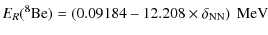
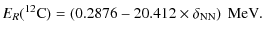
Second, concerning 8Be and 12C, we can extract the sensitivity of ER(8Be) and ER(12C). They scale as
|
(9) |
and
|
(10) |
The numerical results for the sensitivities of
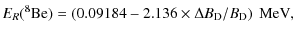
|
(11) | |
|
(12) |
It follows that the energy of the Hoyle level with respect to the
To estimate the effect of
It is appropriate at this point to further note that within
the limits of variation in
![]() that we are considering here,
the effect on promoting the stability of
dineutron or diproton states is negligible. Working within the context
of the same nuclear model, we estimate that a value of
that we are considering here,
the effect on promoting the stability of
dineutron or diproton states is negligible. Working within the context
of the same nuclear model, we estimate that a value of
![]() (for the dineutron) or
(for the dineutron) or ![]() (for the diproton), would be required in order to induce
stability for the dineutron or diproton respectively. As such,
we can safely ignore their potential effects on our results.
(for the diproton), would be required in order to induce
stability for the dineutron or diproton respectively. As such,
we can safely ignore their potential effects on our results.
3.3
Sensitivity
of the -reaction
rate
The method described above provides a consistent way to evaluate the
sensitivity of the ![]() -reaction
rate to a variation of the constants. This rate has been computed
numerically as explained in Angulo
et al. (1999) and as described in Appendix B where both an
analytical approximation valid for sharp resonances and a numerical
integration are performed.
-reaction
rate to a variation of the constants. This rate has been computed
numerically as explained in Angulo
et al. (1999) and as described in Appendix B where both an
analytical approximation valid for sharp resonances and a numerical
integration are performed.
The variation in the partial widths of both reactions have
been computed in Appendix B and are depicted in Fig. A.1. Together with
the results of the previous section and the details of the
Appendix B, we can compute the ![]() -reaction rate as a function
of temperature and
-reaction rate as a function
of temperature and
![]() .
This is summarised in Fig. 3
which compares the rate for different values of
.
This is summarised in Fig. 3
which compares the rate for different values of
![]() to the NACRE rate (Angulo
et al. 1999), which is our reference when no
variation of constants is assumed (i.e.
to the NACRE rate (Angulo
et al. 1999), which is our reference when no
variation of constants is assumed (i.e.
![]() ). One can also refer to
Fig. B.1
which compares the full numerical integration to the analytical
estimation (2)
which turns out to be excellent in the range of temperatures of
interest. As one can see, for positive values of
). One can also refer to
Fig. B.1
which compares the full numerical integration to the analytical
estimation (2)
which turns out to be excellent in the range of temperatures of
interest. As one can see, for positive values of
![]() ,
the resonance energies are lower, so that the
,
the resonance energies are lower, so that the ![]() process
is more efficient (see Appendix B).
process
is more efficient (see Appendix B).
![\begin{figure}
\par\includegraphics[width=8.8cm,clip]{13684fig03.eps}
\end{figure}](/articles/aa/full_html/2010/06/aa13684-09/img119.png)
|
Figure 3:
The ratio between the 3 |
| Open with DEXTER | |
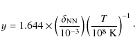
Let us compare the result of Fig. 3, which gives
![]() to a simple estimate. Using the analytic expression (2) for the reaction
rate, valid only for a sharp resonance, y is
simply given by
to a simple estimate. Using the analytic expression (2) for the reaction
rate, valid only for a sharp resonance, y is
simply given by

|
(15) |
where the sensitivity
|
(16) |
This gives the correct order of magnitude for the curves depicted in Fig. 3 as well as their scalings with
The sensitivity to a variation in the intensity of the
N-N interaction arises from the fact that
![]() .
That the typical correction to the resonant energies is of the order of
10 MeV (
.
That the typical correction to the resonant energies is of the order of
10 MeV (
![]() ),
compared to the resonant energies themselves which are around
0.1 MeV, allows one to put relatively strong constraints on
any variation. This is reminiscent of the case of the resonance
producing an excited state of 150Sm of
importance in setting constraints on the variation in couplings using
the Oklo reactor (Fujii et al. 2000; Olive
et al. 2002; Shlyakhter 1976; Damour &
Dyson 1996; Petrov
et al. 2006). In that case, the resonant
energy is 0.1 eV compared to corrections of about
1 MeV due to changes in the fine structure constant, leading
to limits on
),
compared to the resonant energies themselves which are around
0.1 MeV, allows one to put relatively strong constraints on
any variation. This is reminiscent of the case of the resonance
producing an excited state of 150Sm of
importance in setting constraints on the variation in couplings using
the Oklo reactor (Fujii et al. 2000; Olive
et al. 2002; Shlyakhter 1976; Damour &
Dyson 1996; Petrov
et al. 2006). In that case, the resonant
energy is 0.1 eV compared to corrections of about
1 MeV due to changes in the fine structure constant, leading
to limits on
![]() of the order of 10-7.
of the order of 10-7.
3.4 Using the Deuterium binding energy as a link to fundamental constants
The nuclear model described above introduces the parameter
![]() which is itself not directly related to a set of fundamental constants
such as gauge and Yukawa couplings. In order to make such a connection,
we make use of previous analyses relating the deuterium binding energy
which is itself not directly related to a set of fundamental constants
such as gauge and Yukawa couplings. In order to make such a connection,
we make use of previous analyses relating the deuterium binding energy ![]() to fundamental constants.
to fundamental constants.
Using a potential model, the dependence of ![]() on the nucleon,
on the nucleon, ![]() -meson
and
-meson
and ![]() -meson has
been estimated (Flambaum
& Shuryak 2002; Dmitriev & Flambaum 2003; Flambaum &
Shuryak 2003; Damour
& Donoghue 2008; Coc et al. 2007; Dmitriev
et al. 2004). Furthermore, using the quark matrix
elements for the nucleon, variations in
-meson has
been estimated (Flambaum
& Shuryak 2002; Dmitriev & Flambaum 2003; Flambaum &
Shuryak 2003; Damour
& Donoghue 2008; Coc et al. 2007; Dmitriev
et al. 2004). Furthermore, using the quark matrix
elements for the nucleon, variations in ![]() can be related to variations in the light quark masses (particularly
the strange quark) and thus to the corresponding quark Yukawa couplings
and Higgs vev, v. The remaining sensitivity of
can be related to variations in the light quark masses (particularly
the strange quark) and thus to the corresponding quark Yukawa couplings
and Higgs vev, v. The remaining sensitivity of ![]() to a dimensionful quantity is ascribed to the QCD scale
to a dimensionful quantity is ascribed to the QCD scale ![]() .
In Coc et al. (2007),
it was concluded that
.
In Coc et al. (2007),
it was concluded that
|
(17) |
Eq. (8) can then link any constraint on
Further relations are possible in the context of unified theories of
gauge interactions. From the low energy expression for
![]() ,
,
|
(18) |
one can determine the relation between the changes in
Typical values for R are of order 30 in many grand unified theories, but there is considerable model dependence in this coefficient (Dine et al. 2003).
![\begin{figure}
\par\includegraphics[width=8cm,clip]{13684fig04.eps}\hspace*{0.3cm}
\includegraphics[width=8.4cm,clip]{13684fig05.eps}
\end{figure}](/articles/aa/full_html/2010/06/aa13684-09/img135.png)
|
Figure 4:
Left panel: HR diagrams for 15 |
| Open with DEXTER | |
Furthermore, in theories in which the electroweak scale is derived by
dimensional transmutation, changes in the Yukawa couplings
(particularly the top Yukawa) leads to exponentially large changes in
the Higgs vev. In such theories,

with
Finally, using the relations in Eqs. (19)
and (20),
we can write
If in addition, we relate the gauge and Yukawa couplings through
An alternative investigation (Yoo & Scherrer 2003; Beane & Savage 2003; Epelbaum et al. 2003) suggests a large dependence of

|
(23) |
where r is expected to range between 6 and 10. Again, this allows one to related
As these two examples demonstrate, the main problem arises from the difficulty to determine the role of the QCD parameter in low energy nuclear physics. They show, however, that such a link can be drawn, even though it is strongly model-dependent.
4 Stellar implications
The Geneva stellar code was adapted to take into account the reaction
rates computed above. The version of the code we use is the one
described in Ekström et al.
(2008). Here, we only consider models of 15 ![]() and 60
and 60 ![]() without rotation and assume an initial chemical composition given by X=
0.7514, Y= 0.2486 and Z=0. This
corresponds to the BBN abundance of He at the baryon density determined
by WMAP (Komatsu et al. 2009)
and at zero metallicity as is expected to be appropriate for
Population III stars. For 16 values of the free
parameter
without rotation and assume an initial chemical composition given by X=
0.7514, Y= 0.2486 and Z=0. This
corresponds to the BBN abundance of He at the baryon density determined
by WMAP (Komatsu et al. 2009)
and at zero metallicity as is expected to be appropriate for
Population III stars. For 16 values of the free
parameter
![]() in the range
in the range
![]() ,
we computed a stellar model which was followed up to the end of core
He burning (CHeB). As we will see, beyond this range
in
,
we computed a stellar model which was followed up to the end of core
He burning (CHeB). As we will see, beyond this range
in
![]() ,
stellar nucleosynthesis is unacceptably altered. Note that for some of
the most extreme cases, the set of nuclear reactions now
implemented in the code should probably be adapted for a computation of
the advanced evolutionary phases.
,
stellar nucleosynthesis is unacceptably altered. Note that for some of
the most extreme cases, the set of nuclear reactions now
implemented in the code should probably be adapted for a computation of
the advanced evolutionary phases.
Focusing on the limited range in
![]() will allow us to study the impact of a change of the fundamental
constants on the production of carbon and oxygen in Pop III
massive stars. In this context, we recall that the observations of the
most iron poor stars in the halo offer a wonderful tool to probe the
nucleosynthetic impact of the first massive stars in the Universe.
Indeed these halo stars are believed to form from material enriched by
the ejecta of the first stellar generations in the Universe. Their
surface chemical composition (at least on the Main Sequence),
still bear the mark of the chemical composition of the cloud from which
they formed and thus allow us to probe the nucleosynthetic signature of
the first stellar generations. Any variation of the fundamental
constants which for instance would prevent the synthesis of carbon
and/or oxygen would be very hard to conciliate with present day
observations of the most iron poor stars. For instance the two most
iron poor stars (Frebel
et al. 2008; Christlieb et al. 2004)
both show strong overabundances of carbon and oxygen with respect
to iron.
will allow us to study the impact of a change of the fundamental
constants on the production of carbon and oxygen in Pop III
massive stars. In this context, we recall that the observations of the
most iron poor stars in the halo offer a wonderful tool to probe the
nucleosynthetic impact of the first massive stars in the Universe.
Indeed these halo stars are believed to form from material enriched by
the ejecta of the first stellar generations in the Universe. Their
surface chemical composition (at least on the Main Sequence),
still bear the mark of the chemical composition of the cloud from which
they formed and thus allow us to probe the nucleosynthetic signature of
the first stellar generations. Any variation of the fundamental
constants which for instance would prevent the synthesis of carbon
and/or oxygen would be very hard to conciliate with present day
observations of the most iron poor stars. For instance the two most
iron poor stars (Frebel
et al. 2008; Christlieb et al. 2004)
both show strong overabundances of carbon and oxygen with respect
to iron.
Our results for 15 ![]() and 60
and 60 ![]() stars are presented in Sects. 4.1
and 4.2
respectively.
stars are presented in Sects. 4.1
and 4.2
respectively.
4.1 15 M
 mass star
Figure 4
(left panel) shows the HR diagram for the models
with ![]() between -0.009 et +0.006 in increments of 0.001 (from left to right)
and the right panel shows the central temperature at the moment of the
CNO-cycle ignition (lower curve). On the zero-age main sequence (ZAMS),
the standard (
between -0.009 et +0.006 in increments of 0.001 (from left to right)
and the right panel shows the central temperature at the moment of the
CNO-cycle ignition (lower curve). On the zero-age main sequence (ZAMS),
the standard (
![]() )
model has not yet produced enough 12C to be
able to rely on the CNO cycle, so it starts by
continuing its initial contraction until the CNO cycle
ignites. In this model, CNO ignition occurs when the
central H mass fraction reaches 0.724, i.e. when less
than 3% of the initial H has been burned. Models with
)
model has not yet produced enough 12C to be
able to rely on the CNO cycle, so it starts by
continuing its initial contraction until the CNO cycle
ignites. In this model, CNO ignition occurs when the
central H mass fraction reaches 0.724, i.e. when less
than 3% of the initial H has been burned. Models with
![]() start the ZAMS at the same position as in the standard case, but the
lower 3
start the ZAMS at the same position as in the standard case, but the
lower 3![]() rate yields a phase of contraction which is longer for lower
rate yields a phase of contraction which is longer for lower
![]() (i.e. larger
(i.e. larger
![]() ):
in these models, the less efficient 3
):
in these models, the less efficient 3![]() rates need a
higher
rates need a
higher ![]() to produce enough 12C for triggering the
CNO cycle. The tracks in the HR diagram follow a
strait up-left-ward line until the ignition of the CNO cycle.
Models with
to produce enough 12C for triggering the
CNO cycle. The tracks in the HR diagram follow a
strait up-left-ward line until the ignition of the CNO cycle.
Models with ![]() (i.e. a higher 3
(i.e. a higher 3![]() rate) are almost directly sustained by the CNO cycle on the
ZAMS: the star can more easily counteract its own gravity and
the initial contraction is stopped earlier. Their HR tracks are more
typical. Once the CNO cycle has been triggered, the Main
Sequence (MS) tracks follow the usual up-right-ward direction, keeping
the initial shift towards cooler
rate) are almost directly sustained by the CNO cycle on the
ZAMS: the star can more easily counteract its own gravity and
the initial contraction is stopped earlier. Their HR tracks are more
typical. Once the CNO cycle has been triggered, the Main
Sequence (MS) tracks follow the usual up-right-ward direction, keeping
the initial shift towards cooler
![]() for increasing
for increasing
![]() .
There is a difference of about 0.20 dex between the two
extreme models. Thus, for increasing
.
There is a difference of about 0.20 dex between the two
extreme models. Thus, for increasing
![]() ,
H burning occurs at lower
,
H burning occurs at lower ![]() and
and ![]() (Fig. 4,
right), i.e. at a slower pace. The
MS lifetime,
(Fig. 4,
right), i.e. at a slower pace. The
MS lifetime, ![]() , is
sensitive to the pace at which H is burned, so it increases
with
, is
sensitive to the pace at which H is burned, so it increases
with ![]() .
The relative difference between the standard model MS lifetime
.
The relative difference between the standard model MS lifetime
![]() at
at
![]() and
and
![]() at
at ![]() (+0.006) amounts to -17% (+19%).
(+0.006) amounts to -17% (+19%).
Table 2:
Characteristics of the 15 ![]() models with varying
models with varying ![]() at the end of core He burning.
at the end of core He burning.
While the differences in the 3![]() rates do not lead to strong effects in the evolution characteristics on
the MS, the CHeB phase amplifies the differences between the
models. The upper curve of Fig. 4 (right)
shows the central temperature at the beginning of CHeB. There is a
factor of 2.8 in temperature between the models with
rates do not lead to strong effects in the evolution characteristics on
the MS, the CHeB phase amplifies the differences between the
models. The upper curve of Fig. 4 (right)
shows the central temperature at the beginning of CHeB. There is a
factor of 2.8 in temperature between the models with
![]() and +0.006. To get an idea of what this difference represents,
we can relate these temperatures to the grid of Pop III models
computed by Marigo et al. (2001).
The 15
and +0.006. To get an idea of what this difference represents,
we can relate these temperatures to the grid of Pop III models
computed by Marigo et al. (2001).
The 15 ![]() model with
model with ![]() starts its CHeB at a higher temperature than a standard 100
starts its CHeB at a higher temperature than a standard 100 ![]() of the same stage. In contrast, the model with
of the same stage. In contrast, the model with
![]() starts its CHeB phase with a lower temperature than a standard
12
starts its CHeB phase with a lower temperature than a standard
12 ![]() star at CNO ignition. Table 2 presents the
characteristics of the models for each value of
star at CNO ignition. Table 2 presents the
characteristics of the models for each value of
![]() at the end of CHeB. From these
characteristics, we distinguish four
different cases (see the last column of Table 2 and Fig. 5):
at the end of CHeB. From these
characteristics, we distinguish four
different cases (see the last column of Table 2 and Fig. 5):
![\begin{figure}
\par\includegraphics[width=8.8cm,clip]{13684fig06.eps}
\end{figure}](/articles/aa/full_html/2010/06/aa13684-09/img154.png)
|
Figure 5:
The evolution of the central mass fraction for the main chemical
species inside the core of the 15 |
| Open with DEXTER | |
- I
- In the standard model and when
 is very close to 0, 12C is
produced during He burning until the central temperature is
high enough for the 12C(,
is very close to 0, 12C is
produced during He burning until the central temperature is
high enough for the 12C(,  )16O reaction
to become efficient: during the last part of the CHeB phase,
the 12C is processed into 16O.
The star ends its CHeB phase with a core composed of a mixture
of 12C and 16O
(see the top left panel of Fig. 5).
)16O reaction
to become efficient: during the last part of the CHeB phase,
the 12C is processed into 16O.
The star ends its CHeB phase with a core composed of a mixture
of 12C and 16O
(see the top left panel of Fig. 5).
- II
- If the 3
rate is weakened (
 ),
12C is produced at a slower pace,
and
),
12C is produced at a slower pace,
and  is high from the beginning of the CHeB phase, so the 12C(, )16O reaction
becomes efficient very early: as soon as some 12C
is produced, it is immediately transformed into 16O.
The star ends its CHeB phase with a core composed mainly of 16O,
without any 12C and with an increasing fraction
of 24Mg for decreasing
(see the bottom left panel of Fig. 5).
is high from the beginning of the CHeB phase, so the 12C(, )16O reaction
becomes efficient very early: as soon as some 12C
is produced, it is immediately transformed into 16O.
The star ends its CHeB phase with a core composed mainly of 16O,
without any 12C and with an increasing fraction
of 24Mg for decreasing
(see the bottom left panel of Fig. 5).
- III
- For still weaker 3
rates (
 ),
the central temperature during CHeB is such that the 16O(, )20Ne(, )24Mg
chain becomes efficient, reducing the final 16O abundance.
The star ends its CHeB phase with a core composed of nearly
pure 24Mg (see the bottom right panel
of Fig. 5).
Because the abundances of both carbon and oxygen are completely
negligible, we do not list the irrelevant value of C/O for these cases.
),
the central temperature during CHeB is such that the 16O(, )20Ne(, )24Mg
chain becomes efficient, reducing the final 16O abundance.
The star ends its CHeB phase with a core composed of nearly
pure 24Mg (see the bottom right panel
of Fig. 5).
Because the abundances of both carbon and oxygen are completely
negligible, we do not list the irrelevant value of C/O for these cases.
- IV
- If the 3
rate is strong (
 ),
12C is very rapidly produced, but
is so low that the 12C(, )16O reaction
can hardly enter into play: 12C is not
transformed into 16O. The star ends its
CHeB phase with a core almost purely composed of 12C
(see the top right panel of Fig. 5).
),
12C is very rapidly produced, but
is so low that the 12C(, )16O reaction
can hardly enter into play: 12C is not
transformed into 16O. The star ends its
CHeB phase with a core almost purely composed of 12C
(see the top right panel of Fig. 5).
Table 2
shows also the core size at the end of CHeB. As in Heger et al. (2000) the CO
core mass, ![]() , is
determined as the mass coordinate where the mass fraction of 4He drops
below 10-3. The mass of the
CO core increases with decreasing
, is
determined as the mass coordinate where the mass fraction of 4He drops
below 10-3. The mass of the
CO core increases with decreasing
![]() ,
the increase amounting to 8% between
,
the increase amounting to 8% between
![]() and -0.009. This effect comes from the higher central
temperature and greater compactness at low
and -0.009. This effect comes from the higher central
temperature and greater compactness at low
![]() .
The same effect was found by other authors (Schlattl et al. 2004;
Tur
et al. 2007). As shown by these authors,
this effect is expected to have an impact on the remnant mass and thus
on the strength of the final explosion.
.
The same effect was found by other authors (Schlattl et al. 2004;
Tur
et al. 2007). As shown by these authors,
this effect is expected to have an impact on the remnant mass and thus
on the strength of the final explosion.
![\begin{figure}
\par\includegraphics[width=8cm,clip]{13684fig07.eps}
\end{figure}](/articles/aa/full_html/2010/06/aa13684-09/img160.png)
|
Figure 6:
The composition of the core at the end of the central
He burning in the 15 |
| Open with DEXTER | |
Table 3:
Characteristics of the 60 ![]() models with varying
models with varying ![]() .
.
4.2 60 M
mass star
As it is widely believed that Pop III stars are massive, we next
present results for 60 ![]() models (at Z=0). The characteristics of
these models for different values of
models (at Z=0). The characteristics of
these models for different values of
![]() are collected in
Table 3.
are collected in
Table 3.
Figure 7
shows the HR diagram for our 60 ![]() models. During the MS, the shift of the tracks in
models. During the MS, the shift of the tracks in
![]() are slightly reduced compared to the 15
are slightly reduced compared to the 15 ![]() models: by 0.18 dex. Also, all the 60
models: by 0.18 dex. Also, all the 60 ![]() models are almost instantly sustained by the CNO cycle on the
ZAMS, so the tracks are just shifted regularly, without
affecting the shape of the tracks. During CHeB, however, the behaviour
we described for the 15
models are almost instantly sustained by the CNO cycle on the
ZAMS, so the tracks are just shifted regularly, without
affecting the shape of the tracks. During CHeB, however, the behaviour
we described for the 15 ![]() models with
models with ![]() is more pronounced in the case of the 60
is more pronounced in the case of the 60 ![]() models: 12C and 16O are
already exhausted at the end of CHeB (case III) for
models: 12C and 16O are
already exhausted at the end of CHeB (case III) for
![]() .
This can be understood because the 12C(
.
This can be understood because the 12C(![]() ,
, ![]() )16O,
the 16O(
)16O,
the 16O(![]() ,
, ![]() )20Ne
and the 20Ne(
)20Ne
and the 20Ne(![]() ,
, ![]() )24Mg reaction
rates, are a factor of 10 to 100 higher than the 3
)24Mg reaction
rates, are a factor of 10 to 100 higher than the 3![]() rate
when log
rate
when log
![]() ,
i.e. when there is still about 5% of helium in the
core. Instead of a CO core, these models are left with an
almost pure 24Mg core.
,
i.e. when there is still about 5% of helium in the
core. Instead of a CO core, these models are left with an
almost pure 24Mg core.
For the 60 ![]() models with
models with ![]() ,
there is still a reasonable abundance of oxygen up to
,
there is still a reasonable abundance of oxygen up to
![]() =
+0.003. At higher values of
=
+0.003. At higher values of
![]() ,
we are again left with a nearly pure carbon core. For numerical
reasons, the model with
,
we are again left with a nearly pure carbon core. For numerical
reasons, the model with
![]() has proven to be very difficult to follow at the end of CHeB and was
stopped before complete He exhaustion. The results for the
60
has proven to be very difficult to follow at the end of CHeB and was
stopped before complete He exhaustion. The results for the
60 ![]() models are summarised in Fig. 8 which shows the
composition of the core at the end of the CHeB phase. As in the case of
the 15
models are summarised in Fig. 8 which shows the
composition of the core at the end of the CHeB phase. As in the case of
the 15 ![]() models, one can clearly see the strong dependence of the core
composition on
models, one can clearly see the strong dependence of the core
composition on
![]() .
.
The effect of varying
![]() on the core size is less clear in the case of the 60
on the core size is less clear in the case of the 60 ![]() models. In some cases, the model undergoes a CNO boost in the
H-burning shell during CHeB, which reduces the core mass
models. In some cases, the model undergoes a CNO boost in the
H-burning shell during CHeB, which reduces the core mass![]() . The occurrence of the
boost does not follow a clear trend with
. The occurrence of the
boost does not follow a clear trend with
![]() .
It appears on the HR diagram as a sudden drop in
luminosity and effective temperature in the redwards evolution during
CHeB (see Fig. 4,
left).
.
It appears on the HR diagram as a sudden drop in
luminosity and effective temperature in the redwards evolution during
CHeB (see Fig. 4,
left).
![\begin{figure}
\par\includegraphics[width=8cm,clip]{13684fig08.eps}\hspace*{0.3cm}
\includegraphics[width=8cm,clip]{13684fig09.eps}
\end{figure}](/articles/aa/full_html/2010/06/aa13684-09/img164.png)
|
Figure 7:
Left panel: HR diagrams for 60 |
| Open with DEXTER | |
4.3 Limits on the variation of the fundamental constants
All of the models considered were followed without any numerical or
evolutionary problem through the MS. The differences in
lifetimes and tracks during this phase are not constraining enough to
allow the exclusion of some range in
![]() between -0.009
and +0.006. However, the CHeB phase
amplifies these differences.
between -0.009
and +0.006. However, the CHeB phase
amplifies these differences.
![\begin{figure}
\par\includegraphics[width=7.7cm,clip]{13684fig10.eps}
\vspace*{-3.5mm}\end{figure}](/articles/aa/full_html/2010/06/aa13684-09/img165.png)
|
Figure 8:
The composition of the core at the end of the central He burning in the
60 |
| Open with DEXTER | |
At the end of CHeB, the models with
![]() for the 15
for the 15 ![]() model and
model and ![]() for the 60
for the 60 ![]() model have virtually no 12C in the
core, which means that the ``standard'' succession of stellar evolution
burning phases will not be respected (see the bottom right
panel of Fig. 5).
These models are also devoid of 16O or 20Ne
as well, leaving us with a nearly pure 24Mg core.
Note that at this phase, the central temperature is close to that which
would allow the 24Mg(
model have virtually no 12C in the
core, which means that the ``standard'' succession of stellar evolution
burning phases will not be respected (see the bottom right
panel of Fig. 5).
These models are also devoid of 16O or 20Ne
as well, leaving us with a nearly pure 24Mg core.
Note that at this phase, the central temperature is close to that which
would allow the 24Mg(![]() ,
, ![]() )20Ne
or 24Mg(
)20Ne
or 24Mg(![]() ,
, ![]() )28Si reactions
to take place. Therefore, there is a possibility that the
nucleosynthetic chain could go on despite its strange evolution.
However, the Geneva code is developed to follow the standard phases of
stellar evolution, making it necessary to be modified before being able
to follow further the evolution in these odd cases.
)28Si reactions
to take place. Therefore, there is a possibility that the
nucleosynthetic chain could go on despite its strange evolution.
However, the Geneva code is developed to follow the standard phases of
stellar evolution, making it necessary to be modified before being able
to follow further the evolution in these odd cases.
The models with ![]() between -0.002 and -0.005 (between -0.002 and -0.004
for the 60
between -0.002 and -0.005 (between -0.002 and -0.004
for the 60 ![]() model) end the CHeB phase with a central abundance of 12C
between 10-4 and 10-7,
which means that the central C-burning phase will be extremely short.
The 20Ne abundance at that stage is comprised
between 0.04 and 0.10, so there will be a short phase of neon
photodisintegration. Moreover, the 16O abundance
ranges between 0.94 and 0.44 so the oxygen fusion phase will be almost
normal. While the succession of the burning phases seems preserved, one
can however suppose that these models will present very different
yields than the standard case with
model) end the CHeB phase with a central abundance of 12C
between 10-4 and 10-7,
which means that the central C-burning phase will be extremely short.
The 20Ne abundance at that stage is comprised
between 0.04 and 0.10, so there will be a short phase of neon
photodisintegration. Moreover, the 16O abundance
ranges between 0.94 and 0.44 so the oxygen fusion phase will be almost
normal. While the succession of the burning phases seems preserved, one
can however suppose that these models will present very different
yields than the standard case with
![]() .
This point could be the subject of a future study. It is
interesting to note here that since the C-burning phase is very short
(because of the very low 12C abundance
at the end of CHeB), the model will not have much time to lose entropy
by neutrinos losses. We can suppose that the iron core will be hotter
and bigger, so the remnant could be a black hole instead of a neutron
star (Schlattl
et al. 2004; Woosley & Weaver 1986).
.
This point could be the subject of a future study. It is
interesting to note here that since the C-burning phase is very short
(because of the very low 12C abundance
at the end of CHeB), the model will not have much time to lose entropy
by neutrinos losses. We can suppose that the iron core will be hotter
and bigger, so the remnant could be a black hole instead of a neutron
star (Schlattl
et al. 2004; Woosley & Weaver 1986).
The models with
![]() end the CHeB phase with larger and larger 12C abundances
for increasing
end the CHeB phase with larger and larger 12C abundances
for increasing ![]() .
The carbon burning phase will thus be much longer for these models
which will lose a lot of energy through neutrino emission.
A more suspicious feature is that the 16O production
becomes negligible or even null for
.
The carbon burning phase will thus be much longer for these models
which will lose a lot of energy through neutrino emission.
A more suspicious feature is that the 16O production
becomes negligible or even null for
![]() (see the top right panel of Fig. 5) (
(see the top right panel of Fig. 5) (![]() +0.004 for
the 60
+0.004 for
the 60 ![]() model). Normally the bulk of the 16O production
occurs during CHeB: during C burning, the 16O abundance
is reduced by 16O(
model). Normally the bulk of the 16O production
occurs during CHeB: during C burning, the 16O abundance
is reduced by 16O(![]() ,
, ![]() )20Ne,
and during Ne burning, only a small fraction is produced by
the photo-disintegration reaction 20Ne(
)20Ne,
and during Ne burning, only a small fraction is produced by
the photo-disintegration reaction 20Ne(![]() ,
, ![]() )16O.
It would thus mean that such stars do not produce any 16O.
This would pose difficulties for explaining the high
O overabundances observed in extremely iron-poor stars found
in the Galactic halo (see Frebel
et al. 2008).
)16O.
It would thus mean that such stars do not produce any 16O.
This would pose difficulties for explaining the high
O overabundances observed in extremely iron-poor stars found
in the Galactic halo (see Frebel
et al. 2008).
From the preceding discussion, if we exclude a core composed
exclusively of 24Mg (case III), we
must reject ![]() for the 15
for the 15 ![]() model. If we consider that a core only composed of 12C
is not acceptable either (case IV), we must reject
model. If we consider that a core only composed of 12C
is not acceptable either (case IV), we must reject
![]() .
If we consider that a reasonable value of C/O must lay close to unity,
we must also reject case II and the allowed range for
.
If we consider that a reasonable value of C/O must lay close to unity,
we must also reject case II and the allowed range for
![]() is further restricted to -0.001 to +0.002. Similarly
for the 60
is further restricted to -0.001 to +0.002. Similarly
for the 60 ![]() model, excluding cases III and IV leads to a limit
model, excluding cases III and IV leads to a limit
![]() .
The more stringent condition on C/O
.
The more stringent condition on C/O ![]() 1 leads to
1 leads to
![]() .
.
5 Discussion
As we have seen in the previous sections, the extreme sensitivity of
the ![]() process
to the resonant energy of the Hoyle state can lead to very different
histories for massive Population III stars.
In particular, we have shown that very slight variations in
the nucleon-nucleon potential (of order a few
process
to the resonant energy of the Hoyle state can lead to very different
histories for massive Population III stars.
In particular, we have shown that very slight variations in
the nucleon-nucleon potential (of order a few
![]() )
can lead to very different core compositions at the end of CHeB. We
identified two cases (III and IV)
corresponding to nearly pure 24Mg or pure 12C cores.
These cases were present in both the 15 and 60
)
can lead to very different core compositions at the end of CHeB. We
identified two cases (III and IV)
corresponding to nearly pure 24Mg or pure 12C cores.
These cases were present in both the 15 and 60 ![]() models studied. Below
models studied. Below
![]() ,
the stars end the CHeB phase with a core that is almost
completely deprived of carbon, oxygen and neon. This comes from the 12C production
by the 3
,
the stars end the CHeB phase with a core that is almost
completely deprived of carbon, oxygen and neon. This comes from the 12C production
by the 3![]() reaction
becoming extremely weak compared to the 12C(
reaction
becoming extremely weak compared to the 12C(![]() ,
, ![]() )16O reaction
(for which we have used the rates of Kunz
et al. 2002). As soon as a little amount of
12C is produced, it is transformed into
16O, which in turn is transformed into 20Ne
and then 24Mg because of the high temperature
and density at which He burning occurs in these models. Above
)16O reaction
(for which we have used the rates of Kunz
et al. 2002). As soon as a little amount of
12C is produced, it is transformed into
16O, which in turn is transformed into 20Ne
and then 24Mg because of the high temperature
and density at which He burning occurs in these models. Above
![]() ,
the models end the CHeB phase devoid of 16O.
,
the models end the CHeB phase devoid of 16O.
We have checked the limiting values for
![]() variation with stellar models in two different mass domains. For the
15
variation with stellar models in two different mass domains. For the
15 ![]() models, the lower limit is slightly larger than for the 60
models, the lower limit is slightly larger than for the 60 ![]() models. This is the result of the fusion phases occurring at
higher
models. This is the result of the fusion phases occurring at
higher ![]() in the more massive stars, at conditions where the 12C(
in the more massive stars, at conditions where the 12C(![]() ,
, ![]() )16O,
16O(
)16O,
16O(![]() ,
, ![]() )20Ne
and 20Ne(
)20Ne
and 20Ne(![]() ,
, ![]() )24Mg reaction
rates are largely dominant over the 3
)24Mg reaction
rates are largely dominant over the 3![]() rate.
A weak 3
rate.
A weak 3![]() reaction
is a bigger handicap in the high mass domain. In contrast, the
upper limit is larger for the 60
reaction
is a bigger handicap in the high mass domain. In contrast, the
upper limit is larger for the 60 ![]() models, because the 3
models, because the 3![]() reaction
rate is a little less extreme at higher
reaction
rate is a little less extreme at higher ![]() .
.
Excluding these cases allows us to set a relatively
conservative limit on
![]() ,
,
A more aggressive limit would also exclude case II in which CHeB ends with a 16O and 20Ne core with little or no 12C. In this case, one could argue
| (25) |
For the remainder of the discussion, we will restrict our attention to the weak limit (24), as our conclusions can be easily scaled to the stronger limit.
The limit in Eq. (24)
stems directly from the variation in
![]() .
Excluding regions III and IV amount to limiting
.
Excluding regions III and IV amount to limiting
![]() to a range 0.3142-0.5100 MeV, or
to a range 0.3142-0.5100 MeV, or
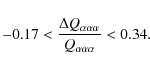
|
(26) |
As discussed in Sect. 3.2, a variation in
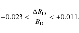
In principle, one would like to next convert the limit on
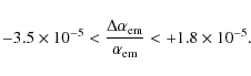
If we further assume the relations between gauge and Yukawa couplings and use Eq. (22), the limit, though more speculative, is actually weakened by a factor of about 2 because of the partial cancellation between the gauge and Yukawa contributions to
The limits on the variation of the fine structure constant
derived above corresponds to a variation of
![]() between the present time and a period around a redshift
between the present time and a period around a redshift
![]() where the Population III stars would have been present. These
values are compatible with the similar limits (also assuming gauge
coupling unification) on the variation of
where the Population III stars would have been present. These
values are compatible with the similar limits (also assuming gauge
coupling unification) on the variation of
![]() at a redshift of 1010 from
BBN predictions. They are larger by a factor of 10
than the values found in the claimed detections (Murphy
et al. 2003; Webb et al. 2001; Murphy
et al. 2007) or a factor of 10 weaker than
the limits from the non-detection (Quast et al. 2004; Srianand
et al. 2004,2007; Chand
et al. 2004) of a variation of
at a redshift of 1010 from
BBN predictions. They are larger by a factor of 10
than the values found in the claimed detections (Murphy
et al. 2003; Webb et al. 2001; Murphy
et al. 2007) or a factor of 10 weaker than
the limits from the non-detection (Quast et al. 2004; Srianand
et al. 2004,2007; Chand
et al. 2004) of a variation of
![]() from quasar absorption systems
at redshifts
from quasar absorption systems
at redshifts ![]() .
.
We remind the reader, that in the present work, the variation
in ![]() is only taken into account for the 3
is only taken into account for the 3![]() reaction.
If the other rates are also affected, the limits found here
would potentially have to be revised, because they have been determined
by anomalies in the evolution that come from a competition between the
efficiency of the various rates. However, being a resonant reaction,
the 3
reaction.
If the other rates are also affected, the limits found here
would potentially have to be revised, because they have been determined
by anomalies in the evolution that come from a competition between the
efficiency of the various rates. However, being a resonant reaction,
the 3![]() reaction is expected to be the most sensitive. Following Oberhummer et al. (2000),
the 16O(
reaction is expected to be the most sensitive. Following Oberhummer et al. (2000),
the 16O(![]() ,
, ![]() )20Ne reaction
is not expected to be sensitive to variations of
)20Ne reaction
is not expected to be sensitive to variations of
![]() ,
while the 12C(
,
while the 12C(![]() ,
, ![]() )16O
could be more affected by such variations because of subthresholds in
the 16O nucleus. According to the same
authors, this last reaction is expected to be strengthened by a
weakening of the nucleon-nucleon interaction. In this case,
the effects described for cases II and III would be
more dramatic than the ones presented here, and so the limits might be
tighter.
)16O
could be more affected by such variations because of subthresholds in
the 16O nucleus. According to the same
authors, this last reaction is expected to be strengthened by a
weakening of the nucleon-nucleon interaction. In this case,
the effects described for cases II and III would be
more dramatic than the ones presented here, and so the limits might be
tighter.
We conclude by asking: is it reasonable to exclude values of
![]() using nucleosynthetic constraints from stellar models? The criteria
that we applied assumes the possibility for a ``normal'' succession of
burning phases (H
using nucleosynthetic constraints from stellar models? The criteria
that we applied assumes the possibility for a ``normal'' succession of
burning phases (H
![]() He
He
![]() C
C
![]() Ne
Ne
![]() O
O
![]() Si). Although we have not done
so here, a modified code
including ``non standard'' fusion phases, would allow us to follow
these models further. It is expected that the resulting yields
would present large anomalies. Given the current state of abundance
determination in extremely metal poor stars, it is highly improbable
that the first stars would not produce fair amounts of 12C
and 16O. The conservative case seem
thus to offer a reasonable limit on the variations of the fundamental
constants.
Si). Although we have not done
so here, a modified code
including ``non standard'' fusion phases, would allow us to follow
these models further. It is expected that the resulting yields
would present large anomalies. Given the current state of abundance
determination in extremely metal poor stars, it is highly improbable
that the first stars would not produce fair amounts of 12C
and 16O. The conservative case seem
thus to offer a reasonable limit on the variations of the fundamental
constants.
Appendix A: Details on the microscopic model
Here, we provide some technical details about the microscopic calculation used to determine the 8Be and 12C binding energies. This calculation is based on the description of the nucleon-nucleon interaction by the Minnesota (MN) force (Thompson et al. 1977), adapted to low-mass systems.
The nuclear part of the interaction potential VN
between nucleons i and j is
given by
![$\displaystyle \left[V_R(r)+\frac{1}{2}(1+P^{\sigma}_{ij})V_{\rm t}(r)
+\frac{1}{2}(1-P^{\sigma}_{ij})V_{\rm s}(r)\right]$](/articles/aa/full_html/2010/06/aa13684-09/img184.png)
![$\displaystyle \times~ \left[\frac{1}{2}u+\frac{1}{2}(2-u)P^{r}_{ij}\right],$](/articles/aa/full_html/2010/06/aa13684-09/img185.png)
where
where energies are expressed in MeV and lengths in fm.
In Eq. (A.1), the exchange-admixture parameter u takes standard value u=1, but can be slightly modified to reproduce important properties of the A-nucleon system (for example, the energy of a resonance). This does not affect the physical properties of the interaction. The MN force is an effective interaction, adapted to cluster models. It is not aimed at perfectly reproducing all nucleon-nucleon properties, as realistic forces used in ab initio models (Navrátil et al. 2009), where the cluster approximation is not employed. The potentials are expressed as Gaussian factors, well adapted to cluster models, where the nucleon orbitals are also Gaussians (Wildermuth & Tang 1977).
![\begin{figure}
\par\includegraphics[width=6cm,clip]{13684fig11.eps}
\end{figure}](/articles/aa/full_html/2010/06/aa13684-09/img192.png)
|
Figure A.1:
The partial widths of 8Be and 12C
as a function of
|
| Open with DEXTER | |
The wave functions (6)
are written in the Resonating Group Method (RGM) which clearly shows
the factorisation of the system wave function in terms of individual
cluster wave functions. In practice the radial wave functions are
expanded over Gaussians, which provides the Generator Coordinate Method
(GCM), fully equivalent to the RGM (Wildermuth
& Tang 1977) but better adapted to numerical
calculations. Some details are given here for the simpler two cluster
case. The radial function
![]() is written as a sum over
Gaussian functions centred at different values
of the Generator Coordinate Rn.
This allows us to write the 8Be wave
function (6) as
is written as a sum over
Gaussian functions centred at different values
of the Generator Coordinate Rn.
This allows us to write the 8Be wave
function (6) as
| (A3) |
where
This development corresponds to a standard expansion on a
variational basis. The binding energies ![]() of the system are obtained by diagonalisation of
of the system are obtained by diagonalisation of
| (A4) |
where the overlap and hamiltonian kernels are defined as
| (A5) |
The Hamiltonian H is given by Eq. (3). Standard techniques exist for the evaluation of these many-body matrix elements (Brink 1966). The choice of the nucleon-nucleon interaction directly affects the calculation of the hamiltonian kernel, and therefore of the eigenenergy
For three-body wave function, the theoretical developments are
identical, but the presentation is complicated by the presence of two
relative coordinates ![]() .
The problem is addressed by using the hyperspherical formalism (Korennov & Descouvemont 2004).
.
The problem is addressed by using the hyperspherical formalism (Korennov & Descouvemont 2004).
Appendix B: Reaction rates and numerical integration
To take into account the (energy dependent) finite widths of the two resonances involved in this two step process, one has to perform numerical integrations as was done in NACRE following Nomoto et al. (1985) and Langanke et al. (1986). Here, the condition of thermal equilibrium is relaxed, but it is assumed that the time scale for alpha capture on 8Be is negligible compared to its lifetime against alpha decay. The rate is calculated as in NACRE for the resonance of interest:
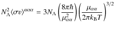
|
||
| (B1) |
where
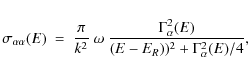
where k is the wave number,
The
![]() rate assumes that 8Be has been formed at an
energy E different from
rate assumes that 8Be has been formed at an
energy E different from
![]() (Langanke et al. 1986).
This rate is given by
(Langanke et al. 1986).
This rate is given by
| |
= | 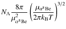
|
|
| (B3) |
where
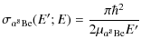
|
||
![$\displaystyle \qquad\qquad \times ~ \frac{\Gamma_{\alpha}(E')
\Gamma_{\gamma}(E...
...E' - E_R(^{12}{\rm C}) + E - E_R(^8{\rm Be})]^2 + \frac{1}{4}
\Gamma (E';E)^2},$](/articles/aa/full_html/2010/06/aa13684-09/img214.png)
|
(B4) |
where the partial widths are those of the Hoyle state and in particular,
However, one must include i) the energy dependence of those widths, away from the resonance energy and ii) the variation in the widths at the resonant energy when this energy changes because of a change in the nuclear interaction.
The energy dependence of the particle widths
![]() is given by:
is given by:
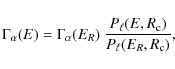
|
(B5) |
where
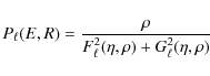
where

is the Sommerfeld parameter.
For radiative capture reactions, the energy dependence of the
gamma width
![]() is given by:
is given by:
|
(B8) |
where
The relevant widths as a function of
![]() are given in Fig. A.1.
They are directly linked to the resulting change of ER(8Be)
and ER(12C).
are given in Fig. A.1.
They are directly linked to the resulting change of ER(8Be)
and ER(12C).
The radiative width,
![]() with its E5 energy
dependence shows little evolution. (The energy of the final
state at 4.44 MeV is assumed to be constant).
In contrast, the 8Be alpha
width undergoes large variations due to the effect of Coulomb barrier
penetrability. Note that compared to these variations, those induced by
a change of
with its E5 energy
dependence shows little evolution. (The energy of the final
state at 4.44 MeV is assumed to be constant).
In contrast, the 8Be alpha
width undergoes large variations due to the effect of Coulomb barrier
penetrability. Note that compared to these variations, those induced by
a change of
![]() in the Coulomb barrier
penetrability (Eqs. (B.7), (B.6))
and
in the Coulomb barrier
penetrability (Eqs. (B.7), (B.6))
and
![]() are considerable smaller.
are considerable smaller.
Numerical integration is necessary at low temperature as the
reaction takes place through the low energy wing of resonances.
It takes even more relative importance, at a given
temperature, when the resonance energy is shifted upwards. On the other
hand, when ![]() increases, the resonance energies decrease, and the
increases, the resonance energies decrease, and the
![]() becomes so small that the numerical integration becomes useless and
soon gives erroneous results because of the finite numerical
resolution. For this reason, when
becomes so small that the numerical integration becomes useless and
soon gives erroneous results because of the finite numerical
resolution. For this reason, when
![]() MeV,
we use instead the Saha equation for the first step and the sharp
resonance approximation for the second step,
i.e. Eq. (2)
when
MeV,
we use instead the Saha equation for the first step and the sharp
resonance approximation for the second step,
i.e. Eq. (2)
when
![]() MeV.
(Note that for high values of
MeV.
(Note that for high values of
![]() ,
the condition
,
the condition
![]() does not hold anymore and
does not hold anymore and
![]() .)
.)
At temperatures in excess of
![]() ,
one must include the contribution of the higher 12C levels
like the one observed by Fynbo
et al. (2005). As this is not of importance
for this study, we just added the contribution given by the last terms
in the NACRE analytical approximation and neglected any
induced variation.
,
one must include the contribution of the higher 12C levels
like the one observed by Fynbo
et al. (2005). As this is not of importance
for this study, we just added the contribution given by the last terms
in the NACRE analytical approximation and neglected any
induced variation.
![\begin{figure}
\par\includegraphics[width=7cm,clip]{13684fig12.eps}
\end{figure}](/articles/aa/full_html/2010/06/aa13684-09/img233.png)
|
Figure B.1:
The 4He(
|
| Open with DEXTER | |
Figure B.1
shows the numerically integrated 4He(
![]() )12C
reaction rates for different values of
)12C
reaction rates for different values of
![]() compared with the analytical approximation (Eq. (2)). The difference
is important at low temperature and small
compared with the analytical approximation (Eq. (2)). The difference
is important at low temperature and small
![]() values but becomes negligible for
values but becomes negligible for
![]()
![]() 0.
At the highest values of
0.
At the highest values of
![]() we consider, the numerical calculation uses the Saha equation for the
first step but the total widths of the 12C level
becomes also too small to be accurately numerically calculated: we use
Eq. (2)
instead.
we consider, the numerical calculation uses the Saha equation for the
first step but the total widths of the 12C level
becomes also too small to be accurately numerically calculated: we use
Eq. (2)
instead.
The 8Be lifetime w.r.t. alpha decay, (
![]() ),
exhibits the opposite behaviour indicating that for large values of
),
exhibits the opposite behaviour indicating that for large values of
![]() it becomes stable. Before that, its lifetime is so long that the 4He(
it becomes stable. Before that, its lifetime is so long that the 4He(
![]() )12C reaction
should be considered as a real two step process with 8Be
included in the network as the assumption that alpha decay is much
faster than alpha capture may not hold anymore. Fortunately, our
network calculations shows that this situation is encountered only for
)12C reaction
should be considered as a real two step process with 8Be
included in the network as the assumption that alpha decay is much
faster than alpha capture may not hold anymore. Fortunately, our
network calculations shows that this situation is encountered only for
![]()
![]() 0.006
for the temperatures and densities considered in our stellar evolution
studies.
0.006
for the temperatures and densities considered in our stellar evolution
studies.
This work was partly supported by i) CNRS PEPS/PTI, ii) CNRS PICS France-USA and by DOE grant DE-FG02-94ER-40823 at the University of Minnesota.
References
- Adams, F. C. 2008, JCAP, 8, 10 [Google Scholar]
- Ajzenberg-Selove, F. 1990, Nucl. Phys. A, 506, 1 [NASA ADS] [CrossRef] [Google Scholar]
- Angulo, C., Arnould, M., Rayet, M., et al. 1999, Nucl. Phys. A, 656, 3 [NASA ADS] [CrossRef] [Google Scholar]
- Ashenfelter, T., Mathews, G. J., & Olive, K. A. 2004a, , 92, 041102 [Google Scholar]
- Ashenfelter, T. P., Mathews, G. J., & Olive, K. A. 2004b, ApJ, 615, 82 [NASA ADS] [CrossRef] [Google Scholar]
- Audi, G., Wapstra, A. H., & Thibault, C. 2003, Nucl. Phys. A, 729, 337 [NASA ADS] [CrossRef] [Google Scholar]
- Barrow, J. D. 1987, Phys. Rev. D, 35, 1805 [NASA ADS] [CrossRef] [Google Scholar]
- Barrow, J. D. 2002, The constants of nature: from alpha to omega (Jonathan Cape) [Google Scholar]
- Beane, S. R., & Savage, M. J. 2003, Nucl. Phys. A, 717, 91 [NASA ADS] [CrossRef] [Google Scholar]
- Bergström, L., Iguri, S., & Rubinstein, H. 1999, Phys. Rev. D, 60, 045005 [NASA ADS] [CrossRef] [Google Scholar]
- Brans, C., & Dicke, R. H. 1961, Phys. Rev., 124, 925 [NASA ADS] [CrossRef] [MathSciNet] [Google Scholar]
- Brink, D. 1966, Proc. Int. School Enrico Fermi, Varenna 1965 (New-York: Academic Press), 36, 247 [Google Scholar]
- Bromm, V., Yoshida, N., Hernquist, L., & McKee, C. F. 2009, Nature, 459, 49 [NASA ADS] [CrossRef] [PubMed] [Google Scholar]
- Calmet, X. 2002, Phys. Lett. B, 540, 173 [NASA ADS] [CrossRef] [Google Scholar]
- Campbell, B. A., & Olive, K. A. 1995, Phys. Lett. B, 345, 429 [NASA ADS] [CrossRef] [Google Scholar]
- Chand, H., Srianand, R., Petitjean, P., & Aracil, B. 2004, A&A, 417, 853 [NASA ADS] [CrossRef] [EDP Sciences] [Google Scholar]
- Christlieb, N., Gustafsson, B., Korn, A. J., et al. 2004, ApJ, 603, 708 [NASA ADS] [CrossRef] [Google Scholar]
- Coc, A., Nunes, N. J., Olive, K. A., Uzan, J.-P., & Vangioni, E. 2007, Phys. Rev. D, 76, 023511 [NASA ADS] [CrossRef] [Google Scholar]
- Cook, C. W., Fowler, W. A., Lauritsen, C. C., & Lauritsen, T. 1957, Phys. Rev., 107, 508 [NASA ADS] [CrossRef] [Google Scholar]
- Csótó, A., Oberhummer, H., & Schlattl, H. 2001, Nucl. Phys. A, 688, 560 [NASA ADS] [CrossRef] [Google Scholar]
- Damour, T., & Esposito-Farese, G. 1992, Class. Quant. Grav., 9, 2093 [NASA ADS] [CrossRef] [Google Scholar]
- Damour, T., & Nordtvedt, K. 1993, , 70, 2217 [Google Scholar]
- Damour, T., & Polyakov, A. M. 1994, Nucl. Phys. B, 423, 532 [NASA ADS] [CrossRef] [MathSciNet] [Google Scholar]
- Damour, T., & Dyson, F. 1996, Nucl. Phys. B, 480, 37 [NASA ADS] [CrossRef] [MathSciNet] [Google Scholar]
- Damour, T., & Donoghue, J. F. 2008, Phys. Rev. D, 78, 014014 [NASA ADS] [CrossRef] [Google Scholar]
- Damour, T., Piazza, F., & Veneziano, G. 2002a, , 89, 081601 [Google Scholar]
- Damour, T., Piazza, F., & Veneziano, G. 2002b, Phys. Rev. D, 66, 046007 [NASA ADS] [CrossRef] [MathSciNet] [Google Scholar]
- Dent, T., & Fairbairn, M. 2003, Nucl. Phys. B, 653, 256 [NASA ADS] [CrossRef] [Google Scholar]
- Dent, T., Stern, S., & Wetterich, C. 2007, Phys. Rev. D, 76, 063513 [NASA ADS] [CrossRef] [Google Scholar]
- Dicke, R. H. 1959, Nature, 183, 170 [NASA ADS] [CrossRef] [Google Scholar]
- Dine, M., Nir, Y., Raz, G., & Volansky, T. 2003, Phys. Rev. D, 67, 015009 [NASA ADS] [CrossRef] [Google Scholar]
- Dirac, P. A. M. 1937, Nature, 139, 323 [NASA ADS] [CrossRef] [Google Scholar]
- Dmitriev, V. F., & Flambaum, V. V. 2003, Phys. Rev. D, 67, 063513 [NASA ADS] [CrossRef] [Google Scholar]
- Dmitriev, V. F., Flambaum, V. V., & Webb, J. K. 2004, Phys. Rev. D, 69, 063506 [NASA ADS] [CrossRef] [Google Scholar]
- Duff, M. J. 2002, unpublished [arXiv:hep-th/0208093] [Google Scholar]
- Duff, M. J., Okun, L. B., & Veneziano, G. 2002, JHEP, 3, 23 [Google Scholar]
- Dunbar, D. N., Pixley, R. E., Wenzel, W. A., & Whaling, W. 1953, Phys. Rev., 92, 649 [NASA ADS] [CrossRef] [Google Scholar]
- Dyson, F. 1972, Aspects of Quantum Theory (Cambridge University Press) [Google Scholar]
- Ekström, S., Meynet, G., Chiappini, C., Hirschi, R., & Maeder, A. 2008, A&A, 489, 685 [NASA ADS] [CrossRef] [EDP Sciences] [Google Scholar]
- Epelbaum, E., Meißner, U., & Glöckle, W. 2003, Nucl. Phys. A, 714, 535 [NASA ADS] [CrossRef] [Google Scholar]
- Fairbairn, M. 1999, unpublished [arXiv:astro-ph/9910328] [Google Scholar]
- Fierz, M. 1956, Helv. Phys. Acta, 29, 128 [Google Scholar]
- Flambaum, V. V., & Shuryak, E. V. 2002, Phys. Rev. D, 65, 103503 [NASA ADS] [CrossRef] [Google Scholar]
- Flambaum, V. V., & Shuryak, E. V. 2003, Phys. Rev. D, 67, 083507 [NASA ADS] [CrossRef] [Google Scholar]
- Flambaum, V. V., & Wiringa, R. B. 2007, Phys. Rev. C, 76, 054002 [NASA ADS] [CrossRef] [Google Scholar]
- Flambaum, V. V., & Wiringa, R. B. 2009, Phys. Rev. C, 79, 034302 [NASA ADS] [CrossRef] [Google Scholar]
- Frebel, A., Collet, R., Eriksson, K., Christlieb, N., & Aoki, W. 2008, ApJ, 684, 588 [NASA ADS] [CrossRef] [Google Scholar]
- Fujii, Y., & Iwamoto, A. 2003, , 91, 261101 [Google Scholar]
- Fujii, Y., Iwamoto, A., Fukahori, T., et al. 2000, Nucl. Phys. B, 573, 377 [NASA ADS] [CrossRef] [Google Scholar]
- Fynbo, H. O. U., Diget, C. A., Bergmann, U. C., et al. 2005, Nature, 433, 136 [NASA ADS] [CrossRef] [PubMed] [Google Scholar]
- Gamow, G. 1967, , 19, 759 [Google Scholar]
- Heger, A., Langer, N., & Woosley, S. E. 2000, ApJ, 528, 368 [NASA ADS] [CrossRef] [Google Scholar]
- Hirschi, R. 2007, A&A, 461, 571 [NASA ADS] [CrossRef] [EDP Sciences] [Google Scholar]
- Hoyle, F. 1954, ApJS, 1, 121 [Google Scholar]
- Ichikawa, K., & Kawasaki, M. 2002, Phys. Rev. D, 65, 123511 [NASA ADS] [CrossRef] [Google Scholar]
- Ichikawa, K., & Kawasaki, M. 2004, Phys. Rev. D, 69, 123506 [NASA ADS] [CrossRef] [Google Scholar]
- Iliadis, C. 2007, Nuclear Physics of Stars (Wenheim, Germany: Wiley-VCH Verlag) [Google Scholar]
- Jordan, P. 1937, Naturwissenschaften, 25, 513 [Google Scholar]
- Jordan, P. 1949, Nature, 164, 637 [NASA ADS] [CrossRef] [Google Scholar]
- Kaluza, T. 1921, Preuss. Akad. Wiss. Berlin (Math. Phys.) K, 1, 966 [Google Scholar]
- Kamimura, M. 1981, Nucl. Phys. A, 351, 456 [NASA ADS] [CrossRef] [Google Scholar]
- Khatri, R., & Wandelt, B. D. 2007, Phys. Rev. Lett., 98, 111301 [NASA ADS] [CrossRef] [Google Scholar]
- Klein, O. 1926, Z. Phys., 37, 895 [Google Scholar]
- Kolb, E. W., Perry, M. J., & Walker, T. P. 1986, Phys. Rev. D, 33, 869 [NASA ADS] [CrossRef] [Google Scholar]
- Komatsu, E., Dunkley, J., Nolta, M. R., et al. 2009, ApJS, 180, 330 [NASA ADS] [CrossRef] [Google Scholar]
- Korennov, S., & Descouvemont, P. 2004, Nucl. Phys. A, 740, 249 [NASA ADS] [Google Scholar]
- Kunz, R., Fey, M., Jaeger, M., et al. 2002, ApJ, 567, 643 [NASA ADS] [CrossRef] [MathSciNet] [Google Scholar]
- Landau, S. J., Mosquera, M. E., & Vucetich, H. 2006, ApJ, 637, 38 [NASA ADS] [CrossRef] [Google Scholar]
- Langacker, P., Segrè, G., & Strassler, M. J. 2002, Phys. Lett. B, 528, 121 [CrossRef] [Google Scholar]
- Langanke, K., Wiescher, M., & Thielemann, F.-K. 1986, Z. Phys. A, 324, 147 [NASA ADS] [Google Scholar]
- Lee, S., Olive, K. A., & Pospelov, M. 2004, Phys. Rev. D, 70, 083503 [NASA ADS] [CrossRef] [Google Scholar]
- Livio, M., Hollowell, D., Truran, J. W., & Weiss, A. 1989, Nature, 340, 281 [NASA ADS] [CrossRef] [Google Scholar]
- Marigo, P., Girardi, L., Chiosi, C., & Wood, P. R. 2001, A&A, 371, 152 [NASA ADS] [CrossRef] [EDP Sciences] [Google Scholar]
- Martins, C. J. A. P., Melchiorri, A., Rocha, G., et al. 2004, Phys. Lett. B, 585, 29 [NASA ADS] [CrossRef] [Google Scholar]
- Müller, C. M., Schäfer, G., & Wetterich, C. 2004, Phys. Rev. D, 70, 083504 [NASA ADS] [CrossRef] [Google Scholar]
- Murphy, M. T., Webb, J. K., & Flambaum, V. V. 2003, MNRAS, 345, 609 [NASA ADS] [CrossRef] [Google Scholar]
- Murphy, M. T., Webb, J. K., & Flambaum, V. V. 2007, , 99, 239001 [Google Scholar]
- Nakashima, M., Nagata, R., & Yokoyama, J. 2008, Prog. Theor. Phys., 120, 1207 [NASA ADS] [CrossRef] [Google Scholar]
- Navrátil, P., Quaglioni, S., Stetcu, I., & Barrett, B. R. 2009, J. Phys. G, 36, 083101 [Google Scholar]
- Nollett, K. M., & Lopez, R. E. 2002, Phys. Rev. D, 66, 063507 [NASA ADS] [CrossRef] [Google Scholar]
- Nomoto, K., Thielemann, F.-K., & Miyaji, S. 1985, A&A, 149, 239 [NASA ADS] [Google Scholar]
- Oberhummer, H., Csótó, A., & Schlattl, H. 2000, Science, 289, 88 [NASA ADS] [CrossRef] [PubMed] [Google Scholar]
- Oberhummer, H., Csótó, A., & Schlattl, H. 2001, Nucl. Phys. A, 689, 269 [NASA ADS] [CrossRef] [Google Scholar]
- Oberhummer, H., Csótó, A., Fairbairn, M., Schlattl, H., & Sharma, M. M. 2003, Nucl. Phys. A, 719, 283 [NASA ADS] [CrossRef] [Google Scholar]
- Olive, K. A., Pospelov, M., Qian, Y., et al. 2002, Phys. Rev. D, 66, 045022 [NASA ADS] [CrossRef] [Google Scholar]
- Olive, K. A., Pospelov, M., Qian, Y., et al. 2004, Phys. Rev. D, 69, 027701 [NASA ADS] [CrossRef] [Google Scholar]
- Petrov, Y. V., Nazarov, A. I., Onegin, M. S., Petrov, V. Y., & Sakhnovsky, E. G. 2006, Phys. Rev. C, 74, 064610 [NASA ADS] [CrossRef] [Google Scholar]
- Pochet, T., Pearson, J. M., Beaudet, G., & Reeves, H. 1991, A&A, 243, 1 [NASA ADS] [Google Scholar]
- Quast, R., Reimers, D., & Levshakov, S. A. 2004, A&A, 415, L7 [NASA ADS] [CrossRef] [EDP Sciences] [Google Scholar]
- Riazuelo, A., & Uzan, J.-P. 2002, Phys. Rev. D, 66, 023525 [NASA ADS] [CrossRef] [MathSciNet] [Google Scholar]
- Rosenband, T., Hume, D. B., Schmidt, P. O., et al. 2008, Science, 319, 1808 [NASA ADS] [CrossRef] [PubMed] [Google Scholar]
- Rozental', I. L. 1988, Big bang, big bounce: how particles and fields drive cosmic evolution (Berlin; New York: Springer-Verlag) [Google Scholar]
- Schlattl, H., Heger, A., Oberhummer, H., Rauscher, T., & Csótó, A. 2004, Ap&SS, 291, 27 [Google Scholar]
- Scóccola, C. G., Mosquera, M. E., Landau, S. J., & Vucetich, H. 2008, ApJ, 681, 737 [NASA ADS] [CrossRef] [Google Scholar]
- Shlyakhter, A. I. 1976, Nature, 264, 340 [NASA ADS] [CrossRef] [Google Scholar]
- Srianand, R., Chand, H., Petitjean, P., & Aracil, B. 2004, Phys. Rev. Lett., 92, 121302 [NASA ADS] [CrossRef] [PubMed] [Google Scholar]
- Srianand, R., Chand, H., Petitjean, P., & Aracil, B. 2007, Phys. Rev. Lett., 99, 239002 [NASA ADS] [CrossRef] [Google Scholar]
- Stefanescu, P. 2007, New Astron., 12, 635 [NASA ADS] [CrossRef] [Google Scholar]
- Suzuki, Y., Matsumura, H., Orabi, M., et al. 2008, Phys. Lett. B, 659, 160 [NASA ADS] [CrossRef] [Google Scholar]
- Taylor, T. R., & Veneziano, G. 1988, Phys. Lett. B, 213, 450 [NASA ADS] [CrossRef] [Google Scholar]
- Thompson, D. R., Lemere, M., & Tang, Y. C. 1977, Nucl. Phys. A, 286, 53 [NASA ADS] [CrossRef] [Google Scholar]
- Tilley, D. R., Kelley, J. H., Godwin, J. L., et al. 2004, Nucl. Phys. A, 745, 155 [NASA ADS] [CrossRef] [Google Scholar]
- Tur, C., Heger, A., & Austin, S. M. 2007, ApJ, 671, 821 [NASA ADS] [CrossRef] [Google Scholar]
- Uzan, J.-P. 1999, Phys. Rev. D, 59, 123510 [NASA ADS] [CrossRef] [Google Scholar]
- Uzan, J.-P. 2003, Rev. Mod. Phys., 75, 403 [NASA ADS] [CrossRef] [Google Scholar]
- Uzan, J. 2004, in Phi in the Sky: The Quest for Cosmological Scalar Fields, ed. C. J. A. P. Martins, P. P. Avelino, M. S. Costa, K. et al., AIP Conf. Ser., 736, 3 [Google Scholar]
- Uzan, J.-P. 2009a, Gen. Rel. Grav., in press [arXiv:0908.2243] [Google Scholar]
- Uzan, J. 2009b, Space Sci. Rev., 21 [Google Scholar]
- Uzan, J., & Leclercq, B. 2008, The Natural Laws of the Universe: Understanding Fundamental Constants (Springer-Verlag) [Google Scholar]
- Webb, J. K., Murphy, M. T., Flambaum, V. V., et al. 2001, Phys. Rev. Lett., 87, 091301 [NASA ADS] [CrossRef] [PubMed] [Google Scholar]
- Weinberg, S. 1983, in Phil. Trans. R. Soc. London Ser. A, 310, 249 [Google Scholar]
- Wetterich, C. 1988, Nucl. Phys. B, 302, 645 [NASA ADS] [CrossRef] [Google Scholar]
- Wetterich, C. 2003, Phys. Lett. B, 561, 10 [NASA ADS] [CrossRef] [Google Scholar]
- Wildermuth, K., & Tang, Y. C. 1977, A unified theory of the nucleus, Vieweg, Braunschweig [Google Scholar]
- Will, C. M. 1993, Theory and Experiment in Gravitational Physics (CUP) [Google Scholar]
- Witten, E. 1984, Phys. Lett. B, 149, 351 [NASA ADS] [CrossRef] [MathSciNet] [Google Scholar]
- Woosley, S. E., & Weaver, T. A. 1986, ARA&A, 24, 205 [NASA ADS] [CrossRef] [Google Scholar]
- Wu, Y., & Wang, Z. 1986, , 57, 1978 [Google Scholar]
- Yoo, J. J., & Scherrer, R. J. 2003, Phys. Rev. D, 67, 043517 [NASA ADS] [CrossRef] [Google Scholar]
Footnotes
- ...
 -factor
![[*]](/icons/foot_motif.png)
- The astrophysical -factor is just the cross
section corrected for the effect of the penetrability of the Coulomb
barrier and other trivial effects.
- ... mass
- We refer the interested reader to Hirschi (2007) or Ekström et al. (2008) for a more detailed description of this phenomenon.
- ...

- We choose
= 1.3
(A11/3
+ A21/3) fm,
for nuclei A1
and A2.
All Tables
Table 1:
Nuclear data for the two steps of the ![]() -reaction.
-reaction.
Table 2:
Characteristics of the 15 ![]() models with varying
models with varying ![]() at the end of core He burning.
at the end of core He burning.
Table 3:
Characteristics of the 60 ![]() models with varying
models with varying ![]() .
.
All Figures
|
|
Figure 1:
Level scheme showing the key levels in the |
| Open with DEXTER | |
| In the text | |
|
|
Figure 2:
Variation in the resonance energies as a function of
|
| Open with DEXTER | |
| In the text | |
|
|
Figure 3:
The ratio between the 3 |
| Open with DEXTER | |
| In the text | |
|
|
Figure 4:
Left panel: HR diagrams for 15 |
| Open with DEXTER | |
| In the text | |
|
|
Figure 5:
The evolution of the central mass fraction for the main chemical
species inside the core of the 15 |
| Open with DEXTER | |
| In the text | |
|
|
Figure 6:
The composition of the core at the end of the central
He burning in the 15 |
| Open with DEXTER | |
| In the text | |
|
|
Figure 7:
Left panel: HR diagrams for 60 |
| Open with DEXTER | |
| In the text | |
|
|
Figure 8:
The composition of the core at the end of the central He burning in the
60 |
| Open with DEXTER | |
| In the text | |
|
|
Figure A.1:
The partial widths of 8Be and 12C
as a function of
|
| Open with DEXTER | |
| In the text | |
|
|
Figure B.1:
The 4He(
|
| Open with DEXTER | |
| In the text | |
Copyright ESO 2010
Current usage metrics show cumulative count of Article Views (full-text article views including HTML views, PDF and ePub downloads, according to the available data) and Abstracts Views on Vision4Press platform.
Data correspond to usage on the plateform after 2015. The current usage metrics is available 48-96 hours after online publication and is updated daily on week days.
Initial download of the metrics may take a while.