| Issue |
A&A
Volume 514, May 2010
|
|
|---|---|---|
| Article Number | A33 | |
| Number of page(s) | 11 | |
| Section | Extragalactic astronomy | |
| DOI | https://doi.org/10.1051/0004-6361/200913612 | |
| Published online | 07 May 2010 | |
Pinning down the ram-pressure-induced halt of star formation in the Virgo cluster spiral galaxy NGC 4388
A joint inversion of spectroscopic and photometric data
C. Pappalardo1 - A. Lançon1 - B. Vollmer1 - P. Ocvirk2 - S. Boissier3 - A. Boselli3
1 - Observatoire astronomique de Strasbourg,
Université de Strasbourg & CNRS UMR 7550, 11 rue de
l'Université, 67000 Strasbourg, France
2 -
Astrophysikalisches Institut Potsdam, An der Sternwarte 16, 14482 Potsdam, Germany
3
- Laboratoire d'Astrophysique de Marseille, OAMP, Université
Aix-Marseille & CNRS UMR6110, 38 rue Frédéric Joliot Curie, 13388
Marseille Cedex 13, France
Received 5 November 2009 / Accepted 20 January 2010
Abstract
Context. In a galaxy cluster, the evolution of spiral
galaxies depends on their cluster environment. Ram pressure due to the
rapid motion of a spiral galaxy within the hot intracluster medium
removes the galaxy's interstellar medium from the outer disk. Once the
gas has left the disk, star formation stops. The passive evolution of
the stellar populations should be detectable in optical spectroscopy
and multi-wavelength photometry.
Aims. The goal of our study is to recover the stripping age of
the Virgo spiral galaxy NGC 4388, i.e. the time elapsed since the
halt of star formation in the outer galactic disk using a combined
analysis of optical spectra and photometry.
Methods. We performed VLT FORS2 long-slit spectroscopy of the
inner star-forming and outer gas-free disk of NGC 4388. We
developed a non-parametric inversion tool that allows us to reconstruct
the star formation history of a galaxy from spectroscopy and
photometry. The tool was tested on a series of mock data using Monte
Carlo simulations. The results from the non-parametric inversion were
refined by applying a parametric inversion method.
Results. The star formation history of the unperturbed galactic
disk is flat. The non-parametric method yields a rapid decline of star
formation ![]() 200 Myr
ago in the outer disk. The parametric method is not able to distinguish
between an instantaneous and a long-lasting star formation truncation.
We find that
200 Myr
ago in the outer disk. The parametric method is not able to distinguish
between an instantaneous and a long-lasting star formation truncation.
We find that
![]() Myr ago the star formation reached half of its pre-stripping value.
Myr ago the star formation reached half of its pre-stripping value.
Conclusions. We are able to give a precise stripping age that is consistent with revised dynamical models.
Key words: galaxies: evolution - galaxies: clusters: individual: Virgo cluster - galaxies: individual: NGC 4388 - Galaxies: stellar content
1 Introduction
Depending on the environment in which they move, spiral galaxies undergo different processes that can modify their structure significantly (see Boselli & Gavazzi 2006 and references therein):
- -
- gravitational effects (e.g. tidal interactions in galaxy-galaxy encounters),
- -
- hydrodynamical effects (e.g. ram pressure stripping or thermal evaporation),
- -
- hybrid processes, i.e. those involving both types of effects, such as preprocessing and starvation.
One important characteristic of Virgo spiral galaxies is their lack of gas (Giovanelli & Haynes 1983; Chamaraux et al. 1980).
The amount of atomic gas in Virgo spirals is up to 80% less than for
field galaxies of the same size and morphological type. Virgo spirals
show truncated HI disks (Giovanelli & Haynes 1983; Cayatte et al. 1990)
with respect to their optical disks. The galaxies on radial orbits are
on average more HI deficient than the ones on circular orbits (Dressler 1986). Chung et al. (2009)
find long HI tails associated with spiral galaxies located at distances
from 0.5 to 1 Mpc from the cluster center. For these cases, ram
pressure stripping is the most probable cause.
The interstellar medium (ISM) of a spiral galaxy that is moving inside
the potential well of a cluster, undergoes pressure due to the
intracluster medium (ICM) that is hot (
![]() K) and tenuous (
K) and tenuous (
![]() atoms cm-3).
If this pressure is higher than the restoring force due to the galactic
potential, the galaxy loses gas from the outer disk. Quantitatively
this is expressed by the Gunn & Gott (1972) criterion:
atoms cm-3).
If this pressure is higher than the restoring force due to the galactic
potential, the galaxy loses gas from the outer disk. Quantitatively
this is expressed by the Gunn & Gott (1972) criterion:
|
(1) |
where
NGC 4388 is a highly inclined Seyfert 2 spiral galaxy (of type Sab) with mB=12.2 mag and a radial velocity of
![]() km s-1 with respect to the cluster mean. It is located at a projected distance of 1.3
km s-1 with respect to the cluster mean. It is located at a projected distance of 1.3
![]() (
(![]() 400 kpc at 16.7 Mpc distance) from the Virgo cluster center (M87). NGC 4388 has lost 85% of its HI gas mass (Cayatte et al. 1990). The HI distribution is strongly truncated within the optical disk. By observing the galaxy in H
400 kpc at 16.7 Mpc distance) from the Virgo cluster center (M87). NGC 4388 has lost 85% of its HI gas mass (Cayatte et al. 1990). The HI distribution is strongly truncated within the optical disk. By observing the galaxy in H![]() Veilleux et al. (1999b) found a large plume of ionized gas extending 4 kpc above the plane. In subsequent SUBARU observations Yoshida et al. (2002) reveal a more extended tail out to 35 kpc to the northeast. Vollmer & Huchtmeier (2003) performed 21-cm line observations with the Effelsberg 100-m radio telescope. They
discovered neutral gas associated with the H
Veilleux et al. (1999b) found a large plume of ionized gas extending 4 kpc above the plane. In subsequent SUBARU observations Yoshida et al. (2002) reveal a more extended tail out to 35 kpc to the northeast. Vollmer & Huchtmeier (2003) performed 21-cm line observations with the Effelsberg 100-m radio telescope. They
discovered neutral gas associated with the H![]() plume out to at least 20 kpc NE of NGC 4388's disk, with an HI mass of
plume out to at least 20 kpc NE of NGC 4388's disk, with an HI mass of
![]() .
With interferometic observations Oosterloo & van Gorkom (2005) show that this HI tail is even
more extended, with a size of
.
With interferometic observations Oosterloo & van Gorkom (2005) show that this HI tail is even
more extended, with a size of
![]() kpc and a mass of
kpc and a mass of
![]() .
.
In the case of NGC 4388, Vollmer & Huchtmeier (2003)
estimate that ram pressure stripping is able to remove more than 80% of
the galaxy's ISM, consistently with the observations of Cayatte et al. (1990). They also estimate that the galaxy passed the cluster center ![]() 120 Myr ago. However this estimation is based on the observations of Vollmer & Huchtmeier (2003). The more extended HI tail found by Oosterloo & van Gorkom (2005) implies that this timescale increases.
120 Myr ago. However this estimation is based on the observations of Vollmer & Huchtmeier (2003). The more extended HI tail found by Oosterloo & van Gorkom (2005) implies that this timescale increases.
Once the gas has left the galactic disk, star formation, which is
ultimately fueled by the neutral hydrogen, stops. Stripping is believed
to progress inwards from the outermost disk on timescales of 108 years, but at any given radius, stripping happens on a shorter timescale.
The stellar populations
then evolve passively, and this is detectable both in optical spectra and in
the photometry. The detailed analysis of the stellar light provides essential
information on the stripping age, i.e. the time elapsed since the halt of
star formation. These constraints are independent of dynamical models and
can be compared to those derived from the gas morphology and kinematics.
Crowl & Kenney (2008) analyze the stellar populations of the gas-free
outer disk of NGC 4388, 5.5 kpc off the center (with our adopted distance
of 16.7 Mpc). They used SparsePak spectroscopy and GALEX photometry. Their
age diagnostics are based on Lick indices and UV fluxes, which they
compare to stellar population synthesis predictions (models of Martins
et al. 2005). Assuming that the past star formation rate in the galaxy
has been constant on long timescales, they conclude the stripping of
the gas from the outer disk occurs
![]() Myr ago.
Our renewed analysis is based on VLT FORS2 long-slit spectroscopy of NGC 4388 taken at two positions:
Myr ago.
Our renewed analysis is based on VLT FORS2 long-slit spectroscopy of NGC 4388 taken at two positions:
- The first slit was pointed at 1.5 kpc from the center, in a gas-normal star-forming region of the disk. We did not take the exact center to avoid bulge contamination.
- The second slit was pointed at 4.5 kpc from the center, just outside the star-forming gas disk.
The spectra were combined with multi-wavelength photometry. The long-term star formation history of the galaxy was obtained using an extension of the non parametric inversion method of Ocvirk et al. (2006). It combined the information provided by the spectroscopic and photometric data to determine the star formation history using minimal constraints on the solutions. The results were then refined using a parametric method that assumes the halt of star formation at the observed outer position in the disk occurs quasi-instantaneously.
The paper is structured as follows. In Sects. 2 and 3 we describe the observations and explain how we extract the photometry that we use as input data. In Sect. 4 we introduce the new approach used in this paper that combines spectral and photometric analysis. In Sects. 5 and 6 we explain the results of this new method in the case of NGC 4388. Finally, in Sect. 7 we give our conclusions and compare our results to previous work.
2 Observations
2.1 Data set
We performed observations of NGC4388 on May 2, 2006 at the European
Southern Observatory Very Large Telescope (VLT) facility on Cerro
Paranal, Chile.
The instrument we used was the FOcal Reducer and low dispersion
Spectrograph 2 (FORS2, Appenzeller et al. 1998) in long-slit spectroscopy observing mode.
The detector system consisted of two 4096 ![]() 2048 CCD.
We chose 2
2048 CCD.
We chose 2 ![]() 2 binning of the pixels (image-scale 0.252''/ binned pixel) and high-gain readout.
We selected grism GRIS-600B with a wavelength range of 3350-6330
2 binning of the pixels (image-scale 0.252''/ binned pixel) and high-gain readout.
We selected grism GRIS-600B with a wavelength range of 3350-6330 ![]() and a resolution of 1.48
and a resolution of 1.48 ![]() / binned pixel. The data were acquired through a 1'' slit, yielding a resolving power of
/ binned pixel. The data were acquired through a 1'' slit, yielding a resolving power of
![]() at the central wavelength.
at the central wavelength.
The two slit positions used for the acquisition are shown in Fig. 1 together with HI contours. Individual exposure times were 600 s for the inner region and 1350 s for the outer. The total integration time for each region were 1800 s and 9450 s (Table 1). We used LTT 4816 and LTT 7987, two white dwarfs with mV=13.96 and mV=12.23, respectively (Bakos et al. 2002; Perryman et al. 1997) as spectrophotometric standards.
![\begin{figure}
\par\includegraphics[width=9cm,clip]{13612_f1.eps}
\end{figure}](/articles/aa/full_html/2010/06/aa13612-09/img30.png)
|
Figure 1: B-band POSSII image of NGC4388 with HI contours. The slit positions for the inner and the outer regions are overlaid. |
| Open with DEXTER | |
Table 1: Journal of observations (ESO program ID 77.B-0039(A)).
Table 2: NGC 4388 photometry.
2.2 Data reduction
Data were reduced with the images and noao.twodspec packages of the Image Reduction and Analysis Facility (IRAF)![]() (Tody 1993).
We created average bias and flat-field images using daytime calibration, and we removed cosmic ray hits using a
(Tody 1993).
We created average bias and flat-field images using daytime calibration, and we removed cosmic ray hits using a ![]() -clipping rejection.
-clipping rejection.
After bias and flat-field correction, we combined the individual galaxy
exposures and applied the wavelength calibration to the spectral axis
of the images.
The aperture used for extracting the 1D spectra covers a length of
32.76'' along the slit for both the inner and the outer regions of NGC
4388.
The sky subtraction was based on a linear fit to the sky windows on
either side of the aperture.
Finally, we used the spectrum of LTT 4816 and its intrinsic fluxes (Hamuy et al. 1992)
to calibrate the flux of the spectra.
The flux calibration is ![]()
![]() accurate, based on the comparison of the energy distributions obtained using either LTT4816 or LTT7987 as a standard.
accurate, based on the comparison of the energy distributions obtained using either LTT4816 or LTT7987 as a standard.
The final reduced spectra for the inner and outer regions are shown in Sect. 5.
The average signal-to-noise ratio per pixel for the inner and outer regions are ![]() 60 and
60 and ![]() 26, respectively, inside the wavelength ranges used in the analysis.
26, respectively, inside the wavelength ranges used in the analysis.
3 Photometry
For the photometry we used the following archive data:
- GALEX (Gil de Paz et al. 2007): FUV and NUV.
- SDSS (Rel. 6, Adelman-McCarthy et al. 2008): u' , g' , r' , i', and z'.
- 2MASS (Skrutskie et al. 2006): J, H, and K.
The archive images were resampled onto the coordinate grid used in FORS2 observations using ALADIN (Bonnarel et al. 2000).
The photometric zero points were derived using the star 2MASS
J122549.86+124047.9 (Table 2).
For the GALEX images, we used the formulae of Morrissey et al. (2007) to convert counts per second (CPS) into AB magnitudes. The defined zero points are accurate to within ![]() (Morrissey et al. 2007). In Table 2 are shown the magnitude and error for the reference star 2MASS
J122549.86+124047.9 (1st-2nd row), the inner region (3rd-4th
row), and the outer regions (5th-6th row). The total uncertainty for
inner and outer regions are shown in 7th and 8th row, respectively. For
the SDSS and 2MASS filters the magnitude are given in AB and Vega
systems, respectively.
(Morrissey et al. 2007). In Table 2 are shown the magnitude and error for the reference star 2MASS
J122549.86+124047.9 (1st-2nd row), the inner region (3rd-4th
row), and the outer regions (5th-6th row). The total uncertainty for
inner and outer regions are shown in 7th and 8th row, respectively. For
the SDSS and 2MASS filters the magnitude are given in AB and Vega
systems, respectively.
The exact locations of the two spectroscopic apertures on the
images were determined by comparing the wavelength-averaged profile
along the FORS2 slits with cuts through the SDSS g'
image. In both cases a clean peak in the cross correlation function
allowed us to identify the slit position to within 1 pixel size.
The GALEX images have a spatial resolution of about 4
![]() .
Light
measured within a 1
.
Light
measured within a 1
![]() aperture is contaminated by neighboring areas,
but this effect is less than the uncertainties already accounted for,
which are large because of low signal levels.
aperture is contaminated by neighboring areas,
but this effect is less than the uncertainties already accounted for,
which are large because of low signal levels.
We estimated the uncertainties on the final magnitudes for the
galaxy apertures from a combination of the uncertainties on the flux
measurements of the reference star (zero point) and those of the
positioning of the slit (see Table 2):
|
(2) |
4 Method
The spectral energy distribution (SED) of a galaxy can be considered as the integrated light produced by different stellar populations with different ages and metallicities. The light and mass contributions of each population depend on the star formation history of the observed region during the galaxy's life.
If we define an initial mass function and a set of isochrones, we can obtain the intrinsic spectrum
![]() of the single stellar population of age t, metallicity Z, and unit mass by integrating over the stellar masses.
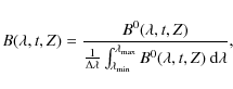
Assuming that the metallicities of the stars can be described by a single-valued age-metallicity relation Z(t), we can derive the unobscured SED of a galaxy at rest:
of the single stellar population of age t, metallicity Z, and unit mass by integrating over the stellar masses.
Assuming that the metallicities of the stars can be described by a single-valued age-metallicity relation Z(t), we can derive the unobscured SED of a galaxy at rest:
in which
Since we observe the light and not the mass in a galaxy, it is more convenient to convert the mass-weighted spectral basis
![]() into a luminosity-weighted basis.
The difference is that
into a luminosity-weighted basis.
The difference is that
![]() defines the spectrum of a single stellar population (SSP) of unit mass, and
defines the spectrum of a single stellar population (SSP) of unit mass, and
![]() defines an SSP spectrum of unit flux.
Instead of mass contributions we deal with light contributions, thus converting the
defines an SSP spectrum of unit flux.
Instead of mass contributions we deal with light contributions, thus converting the
![]() into the luminosity-weighted stellar age distribution (hereafter SAD):
into the luminosity-weighted stellar age distribution (hereafter SAD):
|
(4) |
where
|
(5) |
Eq. (3) becomes
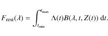
In the same way we can associate a photometric value with each spectrum
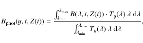
|
(7) |
in which y = [ FUV , NUV , u' , g' , i' , r' , z' , J , H , K], and Ty is the transmission curve associated with each y. Unobscured photometry
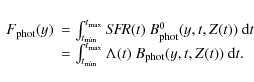
Equation (6) is not complete, because it does not take other effects into account that can modify the final shape of the SED of a galaxy, as follows:

- Extinction: when fitting spectroscopic data we use a flexible
continuum correction that can account both for the reddening due to
dust and for flux calibration errors. The method allows us to use the
information present in the spectral lines without using the continuum
of the spectrum,
which is preferable when the flux calibration is not perfect. In
practice, we define a set of equally spaced anchor points across the
wavelength range of the optical spectra. Their ordinates are then
optimized in such a way that the cubic spline interpolation through the
points cancels out any SED difference
between models and data. We refer to this adjustable correction as NPEC
hereafter (for non parametric estimate of the continuum).
For the photometry, however, extinction must be accounted for explicitly. We adopted the attenuation law of Calzetti (2001) that uses the colour excess E(B-V) as a single parameter (see, however, Sect. 6). -
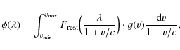
- Radial velocities of the stars: we assumed that the velocities
of stars of all ages along the line of sight have the same velocity
distribution. We can approximate the spectrum of a galaxy as the
convolution of the spectrum at rest and a line of sight velocity
distribution g(v):
where is defined in Eq. (6), and c is the velocity of light.
The integrals in Eqs. (6), (8), and (9) are transformed into discrete sums for numerical treatment.
is defined in Eq. (6), and c is the velocity of light.
The integrals in Eqs. (6), (8), and (9) are transformed into discrete sums for numerical treatment.
- a non parametric method in which we recover the star formation history by resolving the associated inverse problem with regularized methods (see Ocvirk et al. 2006a);
- a parametric method in which we define a set of possible
 depending on one free parameter, the time
elapsed since the stripping event. We then find the most probable solution by minimizing the classical
depending on one free parameter, the time
elapsed since the stripping event. We then find the most probable solution by minimizing the classical  function.
The non parametric method has the advantage of providing the star formation history and trends in the age-metallicity relation of the galaxy with minimal constraints on their shape. On the other hand, the regularization of the problem did not allow us to recover functional forms with large gradients, such as those expected for a ram pressure stripping event. This is why we combined the results from the non-parametric analysis with a parametric analysis.
We chose as SSP library the models of Bruzual & Charlot (2003) that cover a time interval
![]() Gyr, a wavelength range
Gyr, a wavelength range
![]() with an average spectral resolution (FWHM) R = 2000 at optical wavelengths. These SSP spectra are constructed with stellar spectra from Le Borgne et al. (2003). The underlying stellar evolution tracks are those of Alongi et al. (1993), Bressan et al. (1993), Fagotto et al. (1994a), Fagotto et al. (1994b) and Girardi et al. (1996).
with an average spectral resolution (FWHM) R = 2000 at optical wavelengths. These SSP spectra are constructed with stellar spectra from Le Borgne et al. (2003). The underlying stellar evolution tracks are those of Alongi et al. (1993), Bressan et al. (1993), Fagotto et al. (1994a), Fagotto et al. (1994b) and Girardi et al. (1996).
4.1 Non parametric method
The non parametric method used is a modification of STECKMAP![]() (Ocvirk et al. 2006a,b),
extended to deal with spectroscopy and photometry jointly. Assuming
gaussian noise in the data, we estimate the most likely solution by
minimizing the following
(Ocvirk et al. 2006a,b),
extended to deal with spectroscopy and photometry jointly. Assuming
gaussian noise in the data, we estimate the most likely solution by
minimizing the following
![]() function for the star formation history and age-metallicity relation:
function for the star formation history and age-metallicity relation:
in which
 is a vector that includes the SAD, the metallicity evolution, the color excess E(B-V)
for the photometry, the NPEC correction vector for spectral analysis
and a spectral broadening function (BF). The last includes the effects
of the line of sight velocity distribution and the broadening
introduced by the instrumentation.
is a vector that includes the SAD, the metallicity evolution, the color excess E(B-V)
for the photometry, the NPEC correction vector for spectral analysis
and a spectral broadening function (BF). The last includes the effects
of the line of sight velocity distribution and the broadening
introduced by the instrumentation.
-
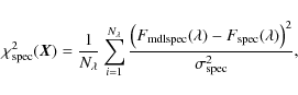
(11)
is the
associated with the spectrum.
 is the model with a defined
and
is the model with a defined
and
 is the observed spectrum,
 is the associated error in the observations, and
 is
the number of points in the spectrum, which we can consider
approximately equal to the number of degrees of freedom of the problem.
is
the number of points in the spectrum, which we can consider
approximately equal to the number of degrees of freedom of the problem.
-
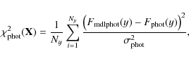
(12)
is the
associated with the photometry, where
 is the model photometry obtained from Eq. (8) with a chosen ,
 are the photometric data and
 are the errors in the measures, and Ny represents the number of bandpasses used.
 -
(13)
is a penalty function needed to regularize the problem. As shown in Ocvirk et al. (2006a), the inverse problem associated with Eqs. (6) and (8) is ill-posed. The function is
chosen to yield high values when the SAD and AMR are a very irregular
function of time or when the BF or the NPEC correction are too chaotic.
The set of
is
chosen to yield high values when the SAD and AMR are a very irregular
function of time or when the BF or the NPEC correction are too chaotic.
The set of
 are adjustable parameters that control the weight of each
in the final estimation.
are adjustable parameters that control the weight of each
in the final estimation.
 determines the relative weights of the photometric and spectroscopic constraints.
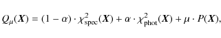
4.2 Parametric method
In this case we assume an exponential star formation history
before the stripping event, a metallicity and a BF, all consistent
with the non parametric results. We reproduce the stripping by a linear decrease in the ![]() on timescales between
on timescales between
![]() Myr. For each of these truncated star formation histories, we calculate the NPEC correction and E(B-V) that produce the lowest
Myr. For each of these truncated star formation histories, we calculate the NPEC correction and E(B-V) that produce the lowest ![]() .
The minimum of
.
The minimum of ![]() is taken to provide the most likely stripping age, which we define as
the time elapsed since star formation has dropped by a factor of two
from its pre-stripping value. The spectroscopic and photometric
contributions to the
is taken to provide the most likely stripping age, which we define as
the time elapsed since star formation has dropped by a factor of two
from its pre-stripping value. The spectroscopic and photometric
contributions to the ![]() are weighted as before:
are weighted as before:
where
5 Results
5.1 Non parametric Inversion
First we point out that the weightings ![]() for the penalty are a central issue of the non parametric method and
that their determination is not a trivial problem. There are different
ways of fixing these values (Titterington 1985). In the case of nonlinear problems, one has to proceed via empirical tuning (Craig & Brown 1986) to define the values of
for the penalty are a central issue of the non parametric method and
that their determination is not a trivial problem. There are different
ways of fixing these values (Titterington 1985). In the case of nonlinear problems, one has to proceed via empirical tuning (Craig & Brown 1986) to define the values of ![]() below which the results present artifacts, and above which the smoothness of the solution is completely due to the penalty.
below which the results present artifacts, and above which the smoothness of the solution is completely due to the penalty.
We chose as penalty functions two finite difference operators (
![]() and
and
![]() in Ocvirk et al. 2006a)
that favor small first derivatives of the AMR and small second
derivatives of the SAD and BF. The penalties for the star formation
history and the metallicity evolution are defined in logarithmic
timescale. We explored the effect of the weight coefficients
in Ocvirk et al. 2006a)
that favor small first derivatives of the AMR and small second
derivatives of the SAD and BF. The penalties for the star formation
history and the metallicity evolution are defined in logarithmic
timescale. We explored the effect of the weight coefficients ![]() through a campaign of inversions of artificial spectra. For the NPEC
correction, we found it was not necessary to require smoothness
explicitely, and the penalization simply acts to normalize the
continuum correction (thus avoiding the degeneracy between the absolute
values of this correction and the star formation rates). The method
recovers similar well-behaved BF for a wide range of
through a campaign of inversions of artificial spectra. For the NPEC
correction, we found it was not necessary to require smoothness
explicitely, and the penalization simply acts to normalize the
continuum correction (thus avoiding the degeneracy between the absolute
values of this correction and the star formation rates). The method
recovers similar well-behaved BF for a wide range of
![]() .
The campaign showed that it is not possible to recover more than a tentative
linear trend in the AMR with the data available to us, and we chose to
simplify the problem with constant metallicity (i.e. large
.
The campaign showed that it is not possible to recover more than a tentative
linear trend in the AMR with the data available to us, and we chose to
simplify the problem with constant metallicity (i.e. large ![]() ).
A realistic metallicity evolution shows a rapid increase at long lookback times and little increase over the past 5 Gyr (Boissier & Prantzos 2000). From our method we derived a time-bin averaged metallicity over a Hubble time
).
A realistic metallicity evolution shows a rapid increase at long lookback times and little increase over the past 5 Gyr (Boissier & Prantzos 2000). From our method we derived a time-bin averaged metallicity over a Hubble time
![]() .
For typical models of Boissier & Prantzos (2000), this mean metallicity is
.
For typical models of Boissier & Prantzos (2000), this mean metallicity is
![]() -0.01 lower than the time-bin averaged metallicity over the past 5 Gyr.
-0.01 lower than the time-bin averaged metallicity over the past 5 Gyr.
For the stellar age distribution, we adopt the smallest ![]() that provides robust solutions, i.e. low sensitivity to the noise in
the data. This choice was based on successive inversions of pseudo-data
with different
that provides robust solutions, i.e. low sensitivity to the noise in
the data. This choice was based on successive inversions of pseudo-data
with different ![]() .
The stability of the results has been tested via Monte Carlo simulations: we added a Gaussian noise with
.
The stability of the results has been tested via Monte Carlo simulations: we added a Gaussian noise with ![]() equal to the noise of the data to the input spectrum and repeated the inversion. In this way we fixed the limits for the
equal to the noise of the data to the input spectrum and repeated the inversion. In this way we fixed the limits for the ![]() value. In the campaign of tests, we also verified that, within
reasonable limits, the shape of the initial guess does not affect the
recovered solution significantly. We ended up taking a semi-analytical
model of Boissier & Prantzos (2000)
as an initial guess for the star formation rate and the age-metallicity
relation, and a constant for the BF and the NPEC correction.
value. In the campaign of tests, we also verified that, within
reasonable limits, the shape of the initial guess does not affect the
recovered solution significantly. We ended up taking a semi-analytical
model of Boissier & Prantzos (2000)
as an initial guess for the star formation rate and the age-metallicity
relation, and a constant for the BF and the NPEC correction.
For each region we reconstructed the star formation history using the VLT spectrum alone (
![]() ), the photometry alone (
), the photometry alone (
![]() )
and spectrum/photometry at the same time (
)
and spectrum/photometry at the same time (
![]() ). In the combined analysis the choice of
). In the combined analysis the choice of
![]() gives, in the final estimation of
gives, in the final estimation of
![]() ,
the same weight to the spectral and photometric analysis. Our conclusions are not significantly affected by the choice of
,
the same weight to the spectral and photometric analysis. Our conclusions are not significantly affected by the choice of ![]() ,
as verified through a campaign of inversions.
,
as verified through a campaign of inversions.
5.1.1 Inner Region
- VLT spectrum (
 .
.
The spectrum shows a fit (top panel in Fig. 2) with
 and a star formation history (Fig. 3) that is approximately flat.
The time-bin averaged metallicity is nearly solar,
and a star formation history (Fig. 3) that is approximately flat.
The time-bin averaged metallicity is nearly solar,
 .
For comparison we took three emission lines ([OII]3727, H
.
For comparison we took three emission lines ([OII]3727, H 4861, [OIII]5007) to recover the metallicity using the strong line method (Pilyugin 2000). We obtained
 consistent with the results of the inversion.
The broadening function is centered on -100 km s-1.
The shift and the width of the broadening function are consistent with
expectation based on galactic rotation and non-circular motions in a
barred potential (Veilleux et al. 1999b).
consistent with the results of the inversion.
The broadening function is centered on -100 km s-1.
The shift and the width of the broadening function are consistent with
expectation based on galactic rotation and non-circular motions in a
barred potential (Veilleux et al. 1999b).
![\begin{figure}
\par\includegraphics[width=16.2cm,clip]{13612_f2a.eps}\vspace*{2m...
...\vspace*{2mm}
\includegraphics[width=16.2cm,clip]{13612_f2c.eps}
\end{figure}](/articles/aa/full_html/2010/06/aa13612-09/Timg95.png)
Figure 2: NGC 4388 inner region fits. Top panel: spectra (black line) and best fit (red line) obtained from inversion with
 .
The bottom of the panel shows the residuals (magenta line) and the
.
The bottom of the panel shows the residuals (magenta line) and the  (green line). The cyan vertical lines show the mask used for emission and sky lines. Middle panel: photometry (black crosses) and best fit (red crosses) obtained from inversion with
 overplotted to the corresponding flux (green dotted line). In the
bottom of the panel are shown the residuals (magenta crosses). Bottom panel: same as the middle panel, but using
overplotted to the corresponding flux (green dotted line). In the
bottom of the panel are shown the residuals (magenta crosses). Bottom panel: same as the middle panel, but using
 .
We do not show the fit of the spectrum for the case
,
because it is indistinguishable by eye from the top panel.
.
We do not show the fit of the spectrum for the case
,
because it is indistinguishable by eye from the top panel.
Open with DEXTER ![\begin{figure}
\par\includegraphics[width = 8.8cm,clip]{13612_f3.eps}
\end{figure}](/articles/aa/full_html/2010/06/aa13612-09/Timg96.png)
Figure 3: Non parametric spectral inversion (
= 0) of the inner region of NGC 4388. Top and middle panel: star formation history (SFH) and luminosity weighted stellar age distribution (LWSAD) vs. lookback time. Bottom panel:
spectral broadening function (BF). In each panel the solid lines shows
the results of the inversion with associated error bars obtained from
30 Monte Carlo simulations. The dashed line shows a constant star
formation rate. All the figures are in arbitrary units.
Open with DEXTER ![\begin{figure}
\par\includegraphics[width = 8.8cm,clip]{13612_f4.eps}
\end{figure}](/articles/aa/full_html/2010/06/aa13612-09/Timg97.png)
Figure 4: Non parametric photometric inversion (
= 1) of the inner region of NGC 4388. Top and bottom panel:
star formation history (SFH) and luminosity-weighted stellar age
distribution (LWSAD) vs. lookback time. For a detailed description see
Fig. 3.
Open with DEXTER - Photometry (
)
The fit reproduces the observations well with a
 (middle panel of Fig. 2).
The star formation history (Fig. 4) is quite similar to the star formation history recovered in the case
,
except in the past 10 Myr. The metallicity is consistent with the
spectroscopic results with larger error bars. From the photometric
inversion we recovered the average reddening of the stars in the
region,
E(B-V) = 0.18.
(middle panel of Fig. 2).
The star formation history (Fig. 4) is quite similar to the star formation history recovered in the case
,
except in the past 10 Myr. The metallicity is consistent with the
spectroscopic results with larger error bars. From the photometric
inversion we recovered the average reddening of the stars in the
region,
E(B-V) = 0.18.
- VLT spectrum + photometry (
)
The fit of the spectrum is essentially identical to the case
,
but we do not show it. The photometry is shown in the bottom panel of Fig. 2. The total
 is intermediate between the two former cases. The star formation
history and the luminosity-weighted stellar age distribution are shown
in Fig. 5.
is intermediate between the two former cases. The star formation
history and the luminosity-weighted stellar age distribution are shown
in Fig. 5.
![\begin{figure}
\par\includegraphics[width = 8.8cm]{13612_f5.eps}
\end{figure}](/articles/aa/full_html/2010/06/aa13612-09/img100.png)
|
Figure 5:
Non parametric combined inversion ( |
| Open with DEXTER | |
5.1.2 Outer region
- VLT spectrum (
We obtain a fit (top panel of Fig. 6) with a
 .
The recovered star formation history (Fig. 7) is flat until a lookback time of
.
The recovered star formation history (Fig. 7) is flat until a lookback time of  200 Myr at most, then it shows a drop, as expected from the ram pressure stripping scenario.
The time-bin averaged metallicity is
200 Myr at most, then it shows a drop, as expected from the ram pressure stripping scenario.
The time-bin averaged metallicity is
 ,
about half of that of the inner region. The broadening function is centered on
,
about half of that of the inner region. The broadening function is centered on  200 km s-1, consistent with galactic rotation (Veilleux et al. 1999b). Its width is dominated by the spectral broadening of the instrument.
- Photometry (
)
The star formation history shows a shape similar to the
case, with a departure from a constant value at a lookback time of 200 Myr at most (Fig. 8). The extinction is
E(B-V) = 0.07 and the
 (middle panel of Fig. 6).
![\begin{figure}
\par\includegraphics[width=16cm,clip]{13612_f6a.eps}\vspace*{2.3m...
...\vspace*{2.3mm}
\includegraphics[width=16cm,clip]{13612_f6c.eps}
\end{figure}](/articles/aa/full_html/2010/06/aa13612-09/Timg104.png)
Figure 6: NGC 4388 outer region fits: top panel: spectra (black) and best fit (red) obtained from inversion with
.
The bottom of the panel
shows the residuals (magenta) and the observational errors (green). The
cyan vertical lines show the mask used for emission and sky lines. Middle panel: photometry of NGC 4388 (black crosses and error bars) and best fit (red crosses) obtained from inversion with
.
The best model spectrum is overplotted. The photometric residuals are also shown (magenta crosses). Bottom panel: same as the middle panel, but using
.
We do not shown the fit of the spectrum for the case
,
because it is indistinguishable by eye from the top panel.
Open with DEXTER - VLT spectrum + Photometry (
)
The total fit (bottom panel of Fig. 6) has a
 .
The spectral fit is very similar to the case
so is not shown.
The total star formation history was flat until 200 Myr ago, then it decreases steeply (Fig. 9). The gas stripping of NGC 4388 truncated the star formation history between 100 and 500 Myr ago.
.
The spectral fit is very similar to the case
so is not shown.
The total star formation history was flat until 200 Myr ago, then it decreases steeply (Fig. 9). The gas stripping of NGC 4388 truncated the star formation history between 100 and 500 Myr ago.
Figures 5-9 compare the recovered star formation history for the inner and the outer regions to a flat star formation. While the inner region shows good agreement, the outer region, somewhere between 100-200 Myr, significantly deviates from a flat star formation history. Since we regularize the inverse problem by requiring the solution to be smooth, instantaneous truncation is rejected by construction. Therefore we cannot assess whether the progressive nature of the decline of the post-stripping star formation is real or if it is a consequence of the penalization. We get back to this point in Sect. 6.2.
- 1.
- provides constraints on the long-term star formation history of the galaxy,
- 2.
- confirms a recent radical change in the star formation history of the outer disk,
- 3.
- does not provide a sharply truncated star formation history.
![\begin{figure}
\par\includegraphics[width = 8.8cm]{13612_f7.eps} %\end{figure}](/articles/aa/full_html/2010/06/aa13612-09/img106.png)
|
Figure 7:
Non parametric spectral inversion ( |
| Open with DEXTER | |
![\begin{figure}
\par\includegraphics[width = 8.8cm]{13612_f8.eps} %\end{figure}](/articles/aa/full_html/2010/06/aa13612-09/img107.png)
|
Figure 8:
Non parametric photometric inversion ( |
| Open with DEXTER | |
![\begin{figure}
\par\includegraphics[width = 8.8cm]{13612_f9.eps} %\end{figure}](/articles/aa/full_html/2010/06/aa13612-09/img108.png)
|
Figure 9:
Non parametric combined inversion ( |
| Open with DEXTER | |
![\begin{figure}
\par\includegraphics[width=7.8cm,clip]{13612_f10a.eps}\vspace*{1....
...}\vspace*{1.5mm}
\includegraphics[width=7.8cm,clip]{13612_f10c.eps}
\end{figure}](/articles/aa/full_html/2010/06/aa13612-09/img109.png)
|
Figure 10:
Parametric inversion of the outer region for an instantaneous star formation truncation. Each panel shows the |
| Open with DEXTER | |
5.2 Parametric inversion
We applied the parametric method to the spectrum of the outer region of NGC 4388 to quantify the time elapsed since star formation dropped by a factor of two from its pre-stripping value, which we call stripping age. For the truncation of star formation, we used star formation rates that decline linearly during 0 to 100 Myr. For the pre-stripping star formation history and metallicity, we used the results of Sect. 5.1. This is essential because, as explained below, the derived stripping age depends on the luminosity-weighted Z and on the ratio of young-to-old stars at the time of stripping. The first point to clarify is the importance of the choice of metallicity evolution in the stripping age determination.
To test the influence of different AMRs on determination of the
stripping age, we used a grid of constant metallicity models, as well
as two AMRs from the galaxy evolution models of Boissier & Prantzos (2000).
We find that the stripping age decreases when the average metallicity
increases. The stripping age of the parametric method is only sensitive
to the metallicity averaged over the past 5 Gyr. Since the
time-bin averaged metallicity from the non-parametric method, which is
averaged over a Hubble time, is lower by
![]() -0.01 (cf. Sect. 5.1), we took a constant metallicity of Z = 0.018 for the parametric method. We studied the
-0.01 (cf. Sect. 5.1), we took a constant metallicity of Z = 0.018 for the parametric method. We studied the ![]() as a function of the stripping age. As done for the non parametric
method, we applied the parametric method to the VLT spectrum, the
photometry alone and then spectrum and photometry together. We find
that the stripping age is independent of the duration of the star
formation truncation. The
as a function of the stripping age. As done for the non parametric
method, we applied the parametric method to the VLT spectrum, the
photometry alone and then spectrum and photometry together. We find
that the stripping age is independent of the duration of the star
formation truncation. The ![]() analysis does not allow different durations of the star formation
truncation to be distinguished. In the following we only discuss the
case of instantaneous truncation.
analysis does not allow different durations of the star formation
truncation to be distinguished. In the following we only discuss the
case of instantaneous truncation.
- VLT spectrum (
)
The top panel of Fig. 10 shows the value of
as a function of the stripping age, yielding a most likely stripping age of 190 Myr.
- Photometry (
)
We obtained a
 (middle panel of Fig. 10) and a stripping age of 190 Myr consistent with the result obtained for the VLT spectrum analysis. We also recovered an
E(B-V) = 0.1, in good agreement with the reddening obtained in the equivalent non parametric problem.
(middle panel of Fig. 10) and a stripping age of 190 Myr consistent with the result obtained for the VLT spectrum analysis. We also recovered an
E(B-V) = 0.1, in good agreement with the reddening obtained in the equivalent non parametric problem.
- VLT spectrum + photometry (
)
The minimum
 is 0.57, and the stripping age is again of 190 Myr (bottom panel of Fig. 10).
6 Discussion
6.1 Uncertainties in the parametric method
In determining of the stripping age, a crucial point is to determine the uncertainty of the result. To clarify this point, we discuss here the influence of the potential sources of errors in the method.
- -
- Monte Carlo simulations
We add a Gaussian noise to the spectral and photometric data, and perform 500 Monte Carlo simulations that way. As expected from statistics, the absolute values of the minimum
vary and the dispersion is
 ,
where N is the number of degrees of freedom (>1700 for the spectroscopic analysis, 7 for the photometric analysis).
However, the location of the minimum in the
curves varies very little.
The error on the stripping age associated with the noise is s20 Myr.
,
where N is the number of degrees of freedom (>1700 for the spectroscopic analysis, 7 for the photometric analysis).
However, the location of the minimum in the
curves varies very little.
The error on the stripping age associated with the noise is s20 Myr.
- -
- Extinction law
The extinction law of Calzetti (2001) was designed to provide a reasonable correction for starburst galaxies. Compared to other laws in the literature, such as the standard Milky Way extinction laws, it is relatively flat. The choice of the extinction law affects the UV-optical colors particularly strongly. However, in the external regions of NGC 4388 from which gas has mostly been removed by ram pressure stripping, the effect of the choice of the extinction law can only be small. As a test, we apply to the model spectra two different extinction laws (Calzetti 2001; Cardelli et al. 1989), and we compare the recovered stripping ages. The results differ by 10 Myr.
- -
- Long-term star formation history
At fixed metallicity, we build families of model spectra with different star formation histories. We consider exponentially decreasing star formation rates (
 )
with timescales
)
with timescales
 ,
and 50 Gyr, as well as a flat
,
and 50 Gyr, as well as a flat  .
The stripping age increases from 100 Myr for
.
The stripping age increases from 100 Myr for  Gyr to 190 Myr for a flat ,
because the ratio of young-to-old stars before the ram pressure
stripping event is higher with flatter star formation rates. Shorter
timescales are excluded, because the corresponding spectra are too
heavily dominated by old stars even before any cut in the
is considered. In our study the long-term star formation history is
constrained strongly by the non parametric inversion of Sect. 5.1.
For a wide range of penalization weights, constant star formation rates
are favored.
The uncertainty on the stripping age obtained when considering only
regular star formation histories consistent with the non parametric
results is reduced to about 10 Myr.
Gyr to 190 Myr for a flat ,
because the ratio of young-to-old stars before the ram pressure
stripping event is higher with flatter star formation rates. Shorter
timescales are excluded, because the corresponding spectra are too
heavily dominated by old stars even before any cut in the
is considered. In our study the long-term star formation history is
constrained strongly by the non parametric inversion of Sect. 5.1.
For a wide range of penalization weights, constant star formation rates
are favored.
The uncertainty on the stripping age obtained when considering only
regular star formation histories consistent with the non parametric
results is reduced to about 10 Myr.
- -
- Metallicity
At fixed star formation, we build sets of model spectra using different metallicity values. The stripping age increases with increasing metallicity. With our study the time-bin averaged metallicity over the last 5 Gyr is established through the non-parametric analysis. The error on the metallicity is
 .
The resulting error on the stripping age is 10 Myr. It is worth
noting that the agreement between the stripping ages determined from
the photometry alone and from the spectroscopy alone is best with the
flat star formation history and the quasi-solar metallicity found by
the non-parametric analysis. With other assumptions, this agreement is
lost.
.
The resulting error on the stripping age is 10 Myr. It is worth
noting that the agreement between the stripping ages determined from
the photometry alone and from the spectroscopy alone is best with the
flat star formation history and the quasi-solar metallicity found by
the non-parametric analysis. With other assumptions, this agreement is
lost.
6.2 Gas dynamics and star formation
The non parametric method fixed an upper limit for the stripping age of
about 100-200 Myr, with a rather unconstrained duration for the
truncation. Numerical simulations (Abadi et al. 1999; Vollmer
et al. 2001; Rödiger & Brüggen 2006) show that the ISM located
at a given distance from the galaxy center is stripped rapidly within a
few 10 Myr. Therefore in the family of possible interpretations of
the outer disk data, we favor a posteriori the scenarios with sharp
truncations, although the timescale of the decline cannot be
constrained with the data presented here. The instantaneous truncation
scenario can only be studied with a parametric method, since the
penalization used in the non-parametric method rejects luminosity
weighted stellar age distributions with sharp variations. A rapid halt
in star formation suggested by the dynamical models can only be studied
with a parametric method, where we make the simplifying assumption that
the gas is stripped
instantaneously. The derived stripping age of 190 Myr is
consistent with the extent of the observed H I
tail (Oosterloo & van Gorkom 2005):
a tail extent of 80 kpc in the plane of the sky and along the line
of sight with the given stripping age leads to a total velocity of ![]() 570 km s-1 and a radial velocity of
570 km s-1 and a radial velocity of ![]() 400 km s-1. The latter corresponds to the
difference between the galaxy's systemic velocity and the velocity of the H I tail (Oosterloo & van Gorkom 2005). The full extent of the H I
tail was not known at the time when Vollmer & Huchtmeier (2003)
presented their dynamical model. Their tail has an extent of
40 kpc
with an associated stripping age of 120 Myr. A new, revised
dynamical model (Vollmer, in prep.) with the observed extent yields a
ram pressure peak
400 km s-1. The latter corresponds to the
difference between the galaxy's systemic velocity and the velocity of the H I tail (Oosterloo & van Gorkom 2005). The full extent of the H I
tail was not known at the time when Vollmer & Huchtmeier (2003)
presented their dynamical model. Their tail has an extent of
40 kpc
with an associated stripping age of 120 Myr. A new, revised
dynamical model (Vollmer, in prep.) with the observed extent yields a
ram pressure peak ![]() 170 Myr ago, consistent with our findings.
170 Myr ago, consistent with our findings.
7 Conclusions
VLT FORS2 spectroscopic observations of the inner star-forming and outer gas-free disk of the Virgo spiral galaxy NGC 4388 have been presented. Previous observations indicate that this galaxy has undergone a recent ram pressure stripping event. Once the galaxy's ISM is stripped by ram pressure star formation stops. We detect this star formation truncation in the spectrum and the multiwavelength photometry of the outer disk region of NGC 4388.
To derive star formation histories we extended the non parametric inversion method of Ocvirk et al. (2006a)
making a joint analysis of spectroscopic and photometric data possible.
The new code was tested on a series of mock data using Monte Carlo
simulations. We find that
the results are stable, once that minimization has converged. The
uncertainties for the young stellar ages (![]() 10 Myr) can be large because of the uncertainties
of stellar models. Whitin reasonable limits, e.g. acceptable
10 Myr) can be large because of the uncertainties
of stellar models. Whitin reasonable limits, e.g. acceptable ![]() ,
the shape and the normalization of the initial guess does not
significantly affect the recovered solution (at a fixed signal-to-noise
ratio).
,
the shape and the normalization of the initial guess does not
significantly affect the recovered solution (at a fixed signal-to-noise
ratio).
The new inversion tool was applied to our spectroscopic and
photometric data for NGC 4388. We explored the effect of different
penalizations in case of spectral analysis, photometric analysis and
combined analysis. The main results are (i) the recovered star
formation history is flat for the inner disk spectrum and (ii) for the
outer disk region the inversion yields a star formation drop at a
lookback time of ![]() 200 Myr at most.
200 Myr at most.
We have introduced a parametric method that refines the determination
of the stripping age, the time elapsed since the star formation has
dropped by a factor of two from its pre-stripping value. Based on the
non parametric results, we assumed a flat star formation before the
stripping event and an almost solar metallicity. We approximated the
effect of gas stripping by cutting or decreasing linearly the star
formation at a different lookback time
![]() Gyr. The obtained set of spectra was compared with the observed spectrum of the outer disk of NGC 4388.
The effect of the potential sources of error in the stripping-age determination were evaluated.
Gyr. The obtained set of spectra was compared with the observed spectrum of the outer disk of NGC 4388.
The effect of the potential sources of error in the stripping-age determination were evaluated.
The parametric method leads to a stripping age for NGC 4388 of ![]()
![]() Myr.
It cannot distinguish between an instantaneous and a longer lasting
star formation truncation. The derived stripping age agrees with the
results of a previous work of Crowl & Kenney (2008) and with revised dynamical models.
Myr.
It cannot distinguish between an instantaneous and a longer lasting
star formation truncation. The derived stripping age agrees with the
results of a previous work of Crowl & Kenney (2008) and with revised dynamical models.
This publication makes use of data products from the Two Micron All Sky Survey, which is a joint project of the University of Massachusetts and the Infrared Processing and Analysis Center/CaliforniaInstitute of Technology, funded by the National Aeronautics and Space Administration and the National Science Foundation.
Funding for the SDSS and SDSS-II has been provided by the Alfred P. Sloan Foundation, the Participating Institutions, the National Science Foundation, the U.S. Department of Energy, the National Aeronautics and Space Administration, the Japanese Monbukagakusho, the Max Planck Society, and the Higher Education Funding Council for England. The SDSS Web Site is http://www.sdss.org/.
We would like to thank D. Munro for freely distributing his Yorick programming language (available at http://www.maumae.net/yorick/doc/index.html). We thank the referee for the useful comments.
References
- Abadi, M. G., Moore, B., & Bower, R. G. 1999, MNRAS, 308, 947 [NASA ADS] [CrossRef] [Google Scholar]
- Adelman-McCarthy, J. K., Agüeros, Marcel A., & Allam, Sahar S. 2008, ApJS, 175, 297 [NASA ADS] [CrossRef] [Google Scholar]
- Alongi, M., Bertelli, G., Bressan, A., et al. 1993, A&AS, 97, 851 [Google Scholar]
- Appenzeller, I., Fricke, K., Fürtig, W., et al. 1998, The Messenger, 94, 1 [NASA ADS] [Google Scholar]
- Bakos, G. Á., Sahu, K. C., & Németh, P. 2002, ApJS, 141, 187 [NASA ADS] [CrossRef] [Google Scholar]
- Boissier, S., & Prantzos, N. 2000, MNRAS, 312, 398 [NASA ADS] [CrossRef] [Google Scholar]
- Bonnarel, F., Fernique, P., Bienaymé, O., et al. 2000, A&AS, 143, 33 [NASA ADS] [CrossRef] [EDP Sciences] [Google Scholar]
- Boselli, A., & Gavazzi, G. 2006, PASP, 118, 517 [NASA ADS] [CrossRef] [Google Scholar]
- Bressan, A., Fagotto, F., Bertelli, G., & Chiosi, C. 1993, A&AS, 100, 647 [NASA ADS] [Google Scholar]
- Bruzual, G., & Charlot, S. 2003, MNRAS, 344, 1000 [NASA ADS] [CrossRef] [Google Scholar]
- Calzetti, D. 2001, PASP, 113, 1449 [NASA ADS] [CrossRef] [Google Scholar]
- Cardelli, J. A., Clayton, G. C., & Mathis, J. S. 1989, ApJ, 345, 245 [NASA ADS] [CrossRef] [Google Scholar]
- Cayatte, V., van Gorkom, J. H., Balkowski, C., & Kotanyi, C. 1990, AJ, 100, 604 [NASA ADS] [CrossRef] [Google Scholar]
- Chamaraux, P., Balkowski, C., & Gerard, E. 1980, A&A, 83, 38 [NASA ADS] [Google Scholar]
- Chung, A., van Gorkom, J. H., Kenney, J. D. P., Crowl, H., & Vollmer, B. 2009, AJ, 138, 1741 [NASA ADS] [CrossRef] [Google Scholar]
- Craig, I. J. D., & Brown, J. C. 1986, Inverse problems in astronomy: A guide to inversion strategies for remotely sensed data, Research supported by SERC (Bristol, England and Boston, MA: Adam Hilger, Ltd.) [Google Scholar]
- Crowl, H. H., & Kenney, J. D. P. 2008, AJ, 136, 1623 [NASA ADS] [CrossRef] [Google Scholar]
- Dressler, A. 1986, ApJ, 301, 35 [NASA ADS] [CrossRef] [Google Scholar]
- Fagotto, F., Bressan, A., Bertelli, G., & Chiosi, C. 1994a, A&AS, 105, 29 [NASA ADS] [Google Scholar]
- Fagotto, F., Bressan, A., Bertelli, G., & Chiosi, C. 1994b, A&AS, 104, 365 [NASA ADS] [Google Scholar]
- Fouqué, P., Solanes, J. M., Sanchis, T., & Balkowski, C. 2001, A&A, 375, 770 [NASA ADS] [CrossRef] [EDP Sciences] [Google Scholar]
- Gil de Paz, A., Boissier, S., Madore, B. F., et al. 2007, ApJS, 173, 185 [NASA ADS] [CrossRef] [Google Scholar]
- Giovanelli, R., & Haynes, M. P. 1983, AJ, 88, 881 [NASA ADS] [CrossRef] [Google Scholar]
- Girardi, L., Bressan, A., Chiosi, C., Bertelli, G., & Nasi, E. 1996, A&AS, 117, 113 [Google Scholar]
- Gunn, J. E., & Gott, J. R. I. 1972, ApJ, 176, 1 [NASA ADS] [CrossRef] [Google Scholar]
- Hamuy, M., Walker, A. R., Suntzeff, N. B., et al. 1992, PASP, 104, 533 [NASA ADS] [CrossRef] [Google Scholar]
- Kenney, J. D. P., Crowl, H., van Gorkom, J., & Vollmer, B. 2004, Recycling Intergalactic and Interstellar Matter, 217, 370 [NASA ADS] [Google Scholar]
- Le Borgne, J.-F., Bruzual, G., Pelló, R., et al. 2003, A&A, 402, 433 [NASA ADS] [CrossRef] [EDP Sciences] [Google Scholar]
- Martins, L. P., González Delgado, R. M., Leitherer, C., Cerviño, M., & Hauschildt, P. 2005, MNRAS, 358, 49 [NASA ADS] [CrossRef] [Google Scholar]
- Morrissey, P., Conrow, T., Barlow, T. A., et al. 2007, ApJS, 173, 682 [NASA ADS] [CrossRef] [Google Scholar]
- Ocvirk, P., Pichon, C., Lançon, A., & Thiébaut, E. 2006a, MNRAS, 365, 46 [NASA ADS] [CrossRef] [Google Scholar]
- Ocvirk, P., Pichon, C., Lançon, A., & Thiébaut, E. 2006b, MNRAS, 365, 74 [NASA ADS] [CrossRef] [Google Scholar]
- Oosterloo, T., & van Gorkom, J. 2005, A&A, 437, L19 [NASA ADS] [CrossRef] [EDP Sciences] [Google Scholar]
- Perryman, M. A. C., Lindegren, L., Kovalevsky, J., et al. 1997, A&A, 323, L49 [NASA ADS] [Google Scholar]
- Pilyugin, L. S. 2000, A&A, 362, 325 [NASA ADS] [Google Scholar]
- Quilis, V., Moore, B., & Bower, R. 2000, Science, 288, 1617 [NASA ADS] [CrossRef] [PubMed] [Google Scholar]
- Roediger, E., & Brüggen, M. 2006, MNRAS, 369, 567 [NASA ADS] [CrossRef] [Google Scholar]
- Roediger, E., & Brüggen, M. 2008, MNRAS, 388, L89 [Google Scholar]
- Schulz, S., & Struck, C. 2001, MNRAS, 328, 185 [NASA ADS] [CrossRef] [Google Scholar]
- Skrutskie, M. F., Cutri, R. M., Stiening, R., et al. 2006, AJ, 131, 1163 [NASA ADS] [CrossRef] [Google Scholar]
- Solanes, J. M., Manrique, A., García-Gómez, C., et al. 2001, ApJ, 548, 97 [NASA ADS] [CrossRef] [Google Scholar]
- Titterington, D. M. 1985, A&A, 144, 381 [NASA ADS] [Google Scholar]
- Tody, D. 1993, Astronomical Data Analysis Software and Systems II, 52, 173 [NASA ADS] [Google Scholar]
- Veilleux, S., Bland-Hawthorn, J., Cecil, G., Tully, R. B., & Miller, S. T. 1999, ApJ, 520, 111 [NASA ADS] [CrossRef] [Google Scholar]
- Veilleux, S., Bland-Hawthorn, J., & Cecil, G. 1999, AJ, 118, 2108 [Google Scholar]
- Vollmer, B., & Huchtmeier, W. 2003, A&A, 406, 427 [NASA ADS] [CrossRef] [EDP Sciences] [Google Scholar]
- Vollmer, B., Cayatte, V., Balkowski, C., & Duschl, W. J. 2001, ApJ, 561, 708 [NASA ADS] [CrossRef] [Google Scholar]
- Warmels, R. H. 1988, A&AS, 72, 57 [NASA ADS] [Google Scholar]
- Yasuda, N., Fukugita, M., & Okamura, S. 1997, ApJS, 108, 417 [NASA ADS] [CrossRef] [Google Scholar]
- Yoshida, M., Yagi, M.; Okamura, S., et al. 2002, ApJ, 567, 118 [NASA ADS] [CrossRef] [Google Scholar]
Footnotes
- ... (IRAF)
![[*]](/icons/foot_motif.png)
- IRAF is distributed by the National Optical Astronomy Observatory, which is operated by the Association of Universities for Research in Astronomy, Inc., under cooperative agreement with the National Science Foundation.
- ... STECKMAP
- http://astro.u-strasbg.fr/ ocvirk/
All Tables
Table 1: Journal of observations (ESO program ID 77.B-0039(A)).
Table 2: NGC 4388 photometry.
All Figures
|
|
Figure 1: B-band POSSII image of NGC4388 with HI contours. The slit positions for the inner and the outer regions are overlaid. |
| Open with DEXTER | |
| In the text | |
![\begin{figure}
\par\includegraphics[width=16.2cm,clip]{13612_f2a.eps}\vspace*{2m...
...\vspace*{2mm}
\includegraphics[width=16.2cm,clip]{13612_f2c.eps}
\end{figure}](/articles/aa/full_html/2010/06/aa13612-09/img95.png)
|
Figure 2:
NGC 4388 inner region fits. Top panel: spectra (black line) and best fit (red line) obtained from inversion with
|
| Open with DEXTER | |
| In the text | |
![\begin{figure}
\par\includegraphics[width = 8.8cm,clip]{13612_f3.eps}
\end{figure}](/articles/aa/full_html/2010/06/aa13612-09/img96.png)
|
Figure 3:
Non parametric spectral inversion ( |
| Open with DEXTER | |
| In the text | |
![\begin{figure}
\par\includegraphics[width = 8.8cm,clip]{13612_f4.eps}
\end{figure}](/articles/aa/full_html/2010/06/aa13612-09/img97.png)
|
Figure 4:
Non parametric photometric inversion ( |
| Open with DEXTER | |
| In the text | |
|
|
Figure 5:
Non parametric combined inversion ( |
| Open with DEXTER | |
| In the text | |
![\begin{figure}
\par\includegraphics[width=16cm,clip]{13612_f6a.eps}\vspace*{2.3m...
...\vspace*{2.3mm}
\includegraphics[width=16cm,clip]{13612_f6c.eps}
\end{figure}](/articles/aa/full_html/2010/06/aa13612-09/img104.png)
|
Figure 6:
NGC 4388 outer region fits: top panel: spectra (black) and best fit (red) obtained from inversion with
|
| Open with DEXTER | |
| In the text | |
|
|
Figure 7:
Non parametric spectral inversion ( |
| Open with DEXTER | |
| In the text | |
|
|
Figure 8:
Non parametric photometric inversion ( |
| Open with DEXTER | |
| In the text | |
|
|
Figure 9:
Non parametric combined inversion ( |
| Open with DEXTER | |
| In the text | |
|
|
Figure 10:
Parametric inversion of the outer region for an instantaneous star formation truncation. Each panel shows the |
| Open with DEXTER | |
| In the text | |
Copyright ESO 2010
Current usage metrics show cumulative count of Article Views (full-text article views including HTML views, PDF and ePub downloads, according to the available data) and Abstracts Views on Vision4Press platform.
Data correspond to usage on the plateform after 2015. The current usage metrics is available 48-96 hours after online publication and is updated daily on week days.
Initial download of the metrics may take a while.