| Issue |
A&A
Volume 514, May 2010
|
|
|---|---|---|
| Article Number | A96 | |
| Number of page(s) | 17 | |
| Section | Celestial mechanics and astrometry | |
| DOI | https://doi.org/10.1051/0004-6361/200913346 | |
| Published online | 27 May 2010 | |
A ring as a model of the main belt in
planetary ephemerides![[*]](/icons/foot_motif.png)
P. Kuchynka1 - J. Laskar1 - A. Fienga1,2 - H. Manche1
1 - Astronomie et Systèmes Dynamiques, IMCCE-CNRS UMR8028, Observatoire
de Paris, UPMC, 77 avenue Denfert-Rochereau, 75014 Paris, France
2 - Observatoire de Besançon-CNRS UMR6213, 41 bis avenue de
l'Observatoire, 25000 Besançon, France
Received 24 September 2009 / Accepted 4 February 2010
Abstract
Aims. We assess the ability of a solid ring to model
a global perturbation induced by several thousands of main-belt
asteroids.
Methods. The ring is first studied in an analytical
framework that provides an estimate of all the ring's parameters
excepting mass. In the second part, numerically estimated perturbations
on the Earth-Mars, Earth-Venus, and Earth-Mercury distances induced by
various subsets of the main-belt population are compared with
perturbations induced by a ring. To account for large uncertainties in
the asteroid masses, we obtain results from Monte Carlo experiments
based on asteroid masses randomly generated according to available data
and the statistical asteroid model.
Results. The radius of the ring is analytically
estimated at 2.8 AU. A systematic comparison of the ring with
subsets of the main belt shows that, after removing the
300 most perturbing asteroids, the total main-belt
perturbation of the Earth-Mars distance reaches on average
246 m on the 1969-2010 time interval. A ring with
appropriate mass is able to reduce this effect
to 38 m. We show that, by removing from the main belt
![]() 240 asteroids
that are not necessarily the most perturbing ones, the corresponding
total perturbation reaches on average 472 m, but the ring is
able to reduce it down to a few meters, thus accounting for more than
99% of the total effect.
240 asteroids
that are not necessarily the most perturbing ones, the corresponding
total perturbation reaches on average 472 m, but the ring is
able to reduce it down to a few meters, thus accounting for more than
99% of the total effect.
Key words: celestial mechanics - ephemerides - minor planets, asteroids: general
1 Introduction
Asteroid perturbations are considered the major obstacle for achieving a satisfactory prediction accuracy in planetary ephemerides. The asteroid problem persists despite the ephemerides being fitted to a variety of highly accurate observations available over almost 40 years. The most constraining observations are tracking data from spacecraft orbiting Mars, which over the past 8 years are available with metric precision. Despite this accuracy, today's ephemerides are unable to extrapolate the Mars ranging data one year into the future with a precision better than 15 m (see Folkner et al. 2008; Fienga et al. 2009). The obstacle to improving the situation is to correctly account for a large number of similar asteroid effects without any accurate knowledge of the asteroid masses. In modern ephemerides, usually about 300 asteroids are modeled individually and the rest of the main-belt is represented by a circular ring. Our objective in this study is to estimate the ability of a ring to model large numbers of asteroids.
In Sect. 2 we set a simple analytical framework and show that a ring is in fact a first-order representation of the main-belt perturbation. Section 3 describes a new implementation of the ring in the INPOP ephemeris (see Fienga et al. 2009). To evaluate the ring model, we chose to compare the perturbation induced by the ring on the Earth-Mars distance with the perturbations induced by a test model containing thousands of asteroids. Section 4 describes the chosen test model that consists of 24635 asteroids assigned each according to the available data with reasonable random mass values. In Sect. 5 the effect of the ring is compared with the perturbation induced by the test model after removing various asteroid subsets. The comparison is repeated for different asteroid masses in Monte-Carlo-like experiments. We are thus able to estimate the number of asteroids that need to be individualized in the asteroid model so the ring is able to satisfactorily represent the remaining global perturbation. We also derive estimates for the amplitude of the global perturbation, together with the corresponding mass of the ring and the amplitude of the residual perturbation unmodeled by the ring. The perturbations on the Earth-Mercury and Earth-Venus distances are considered at the end of the section. Some applications of the obtained results are discussed in Sect. 6.
2 Analytical approach
2.1 Averaging the main belt
The perturbation induced on a planet by the main belt is the sum of the perturbations induced by the asteroids within the belt. Accounting in a model for each asteroid individually involves dealing with a very large number of unknown and highly correlated parameters. In consequence, it is not possible to implement all the individual main-belt asteroids in the model. We show that with some hypotheses the asteroid model can actually be reduced to the average effect of a single object.
Let us consider a main-belt asteroid of mass m'
on a fixed orbit perturbing a planet of mass m. We
denote the classical orbital elements with
![]() .
In this whole section we use the convention of marking the variables
related to the asteroid with a prime and the variables related to the
planet without a prime. We assume that in the main-belt the considered
asteroid is not alone on its orbit, but many other objects with similar
masses are spread uniformly in terms of mean longitude on similar
orbits. It is then possible to average the perturbation of the
considered asteroid over the mean longitude
.
In this whole section we use the convention of marking the variables
related to the asteroid with a prime and the variables related to the
planet without a prime. We assume that in the main-belt the considered
asteroid is not alone on its orbit, but many other objects with similar
masses are spread uniformly in terms of mean longitude on similar
orbits. It is then possible to average the perturbation of the
considered asteroid over the mean longitude ![]() without losing any part of the asteroid's contribution to the main-belt
perturbation. For the sake of simplicity, we also average the
perturbation over the mean longitude of the planet. We are thus left
only with a secular effect.
without losing any part of the asteroid's contribution to the main-belt
perturbation. For the sake of simplicity, we also average the
perturbation over the mean longitude of the planet. We are thus left
only with a secular effect.
Laskar & Robutel
(1995) provide the secular Hamiltonian of the three-body
problem expanded in eccentricity and inclination. In the case where the
semi-major axis of the asteroid is always greater than the semi-major
axis of the planet, the Hamiltonian can be rewritten up to the second
degree as
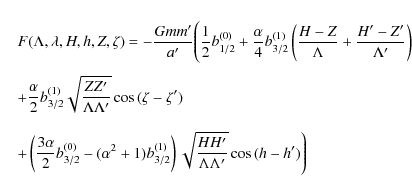
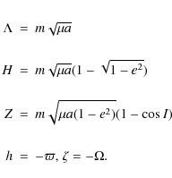
where b1/2(0),b3/2(0),b3/2(1) are Laplace coefficients depending on the semi-major axis ratio
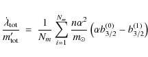
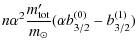
We can calculate the perturbation induced on the planet by the asteroid from Hamilton's equations. By only keeping the lowest order terms in eccentricity and inclination, we get
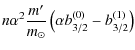
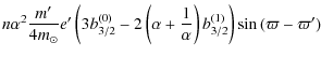
To obtain the perturbation induced by the entire main belt, the above equations have to be summed over all the asteroids. For
where
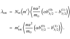
Thus
numerically for all the inner planets. We consider in the catalog only those asteroids with absolute magnitude below 14 and semi-major axis below 3.5 AU. Thus the estimation is based on a total of 24634 orbits. There are actually 24635 asteroids that satisfy these criteria. We eliminated 433 Eros from the selection because its semi-major axis is lower than the semi-major axis of Mars and thus Eqs. (1) do not apply.
The method described to calculate
![]() is applied
also to the other orbital parameters. We thus obtain the
numerical values of
is applied
also to the other orbital parameters. We thus obtain the
numerical values of
![]() ,
,
![]() ,
,
![]() and
and
![]() .
For each inner planet, we can find an average equivalent orbit that
will perfectly fit all the calculated total perturbations. Because
.
For each inner planet, we can find an average equivalent orbit that
will perfectly fit all the calculated total perturbations. Because
![]() is
a monotonously decreasing function of
is
a monotonously decreasing function of ![]() ,
the value of
,
the value of
![]() determines
the semi-major axis of the equivalent orbit unambiguously.
Once the semi-major axis is determined, the calculated values of
determines
the semi-major axis of the equivalent orbit unambiguously.
Once the semi-major axis is determined, the calculated values of
![]() ,
,
![]() determine
the eccentricity and perihelion. Similarly
determine
the eccentricity and perihelion. Similarly
![]() ,
,
![]() determine
the inclination and node. Table 1 summarizes
the orbital parameters of the equivalent orbit obtained on all the
inner planets by averaging the 24634 asteroid orbits. The chosen
reference frame is a nominal invariable plane defined by an inclination
of
determine
the inclination and node. Table 1 summarizes
the orbital parameters of the equivalent orbit obtained on all the
inner planets by averaging the 24634 asteroid orbits. The chosen
reference frame is a nominal invariable plane defined by an inclination
of ![]() and a node at
and a node at ![]() with respect to the International Celestial Reference Frame.
Equations (1)
contain only first-order terms in eccentricities and inclinations.
Because of this approximation, the parameters in Table 1 vary from
one planet to another.
with respect to the International Celestial Reference Frame.
Equations (1)
contain only first-order terms in eccentricities and inclinations.
Because of this approximation, the parameters in Table 1 vary from
one planet to another.
Table 1: Parameters of an averaged orbit representing the main-belt perturbation as determined from the perturbation on the inner planets.
The effects of an orbit averaged over its mean longitude are entirely equivalent to the effects induced by a solid ring. This equivalence has been known since the works of Gauss (see for example Hill 1882) and is valid in both the secular and non-secular cases. For practical purposes, we refer in the following more often to a ring than to the effect of an averaged orbit, but the reader has to bear in mind that both are equivalent.
Although we observe non-zero eccentricity values in Table 1, in this work we study the modeling of the main belt with a circular ring. The non-zero eccentricities are a consequence of the tendency of asteroid perihelia to accumulate close to the longitude of the perihelium of Jupiter. The precession rate of an asteroid perihelium is in fact at its lowest when close to the perihelium of Jupiter. The asteroid perihelia thus spend more time in this region, which explains their apparent accumulation (see Murray & Dermott 1999). For the remainder of this paper we fix the radius of the ring at 2.8 AU. This value is within 0.1 AU of all the radii in Table 1, and it is also the value of the radius of the ring adopted in INPOP06 (Fienga et al. 2008). The initial inclination of the ring with respect to the invariable plane is chosen at zero. This fixes all the ring's geometrical parameters. The only parameter of the main-belt model that is left undetermined is the mass of the ring or equivalently the total mass of the modeled asteroids.
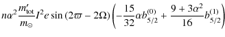
2.2 Perturbation of the orbital elements
We use Eqs. (1)
to obtain analytical expressions of the secular perturbation induced by
a ring on a planet. We stress that, although the analytical results are
presented in the secular case, it is merely for convenience and the
objective in this study is to assess the ring model in the general
non-secular case. By setting e' and I'
at zero one obtains


The ring induces linear drifts in the mean, perihelion, and node longitudes of the planet. There is no secular effect on the semi-major axis because, in the secular case, the Hamiltonian is independent of
In Table 2, we use Eqs. (2) and (3) to quantitatively estimate the effect induced on Earth and Mars by a ring with radius at 2.8 AU and a mass of
Table 2: Secular effect of a ring, with INPOP06 parameters, on the orbital elements of the Earth and Mars.
2.3 Perturbation of the Earth-Mars distance
In this work we focus on the Earth-Mars mutual distance, which today is the most accurately observed parameter. Indeed Mars has been a target for many missions. These provide highly accurate ranging data with accuracies varying from roughly 20 m for the Viking data to accuracies of about 1 m for more recent missions like Mars Global Surveyor, Mars Orbiter, or the ongoing Mars Express mission. We limit our study of the asteroid perturbations to the interval between years 1969 and 2010. This corresponds roughly to the interval spanned by the available ranging data.
Let us denote with ![]() any perturbation induced on the Earth-Mars distance. We have
any perturbation induced on the Earth-Mars distance. We have

where D and D0 are the Earth-Mars distances in the perturbed and unperturbed cases respectively. D and D0 each depend on the perturbed and unperturbed orbital elements of Earth and Mars. By writing a first-order Taylor expansion of D in terms of the perturbations of the individual orbital elements, we obtain
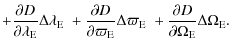
The indexes E and M refer to the Earth and Mars. In the expansion, (

where
We calculated estimates of the partial derivatives by differentiating a second-degree eccentricity and inclination expansion of the Earth-Mars distance. The resulting estimates are functions of approximately constant amplitude oscillating with frequencies close to the Earth-Mars synodic frequency. Table 3 lists the amplitudes of all the partial derivatives. The significant differences among the amplitudes of the partial derivatives stem from the various orders in eccentricity and inclination.
The general expression (4) can be used to estimate the effect induced on the Earth-Mars distance by the ring with INPOP06 parameters. With Table 3 and the values of the secular perturbations calculated in Table 2, we find that the perturbation will reach approximately 5 m over one year, mainly because of the drift in the mean longitude of Mars.
Table 3: The Earth-Mars distance dependence on the orbital elements.
3 Numerical integrations
3.1 The implementation of the ring in INPOP
In Krasinsky et al. (2002) the ring was numerically implemented as a perturbing acceleration in the ecliptic plane of each planet, and this implementation has been adopted in INPOP06 as well. Fienga et al. (2009) show that in long-term integrations the ring causes a slight drift in the Solar System barycenter of approximately 10 m over a century. Indeed with the ring modeled as an exterior force, the system's total linear momentum is not conserved. The existence of this drift motivated a more realistic implementation of the ring adopted since in INPOP08.
The ring is treated as a solid rotating body, which fully interacts with the planets. Although its initial orientation is taken to be parallel to the system's invariable plane, the orientation of the ring is an integrated parameter that evolves with time under the influence of the planetary perturbations. The angular momentum of the ring is constant in amplitude and determined by the radius of the ring and Kepler's law. The linear and angular momenta of the system are thus conserved, which eliminates the barycenter drift occurring in the previous implementation. Because the averaged orbit is bound to the Sun by gravitation, in INPOP we fix the center of the ring to the barycenter of the Sun. We note that a free floating ring centered on the Sun or on the barycenter of the Solar System is actually unstable and would gradually drift away from its initial position. The expression for the force exerted by a ring on a particle is given in Appendix A.
3.2 Comparison with the analytical expressions
![\begin{figure}
\par\includegraphics[width=8.5cm,clip]{13346fg01.eps}
\end{figure}](/articles/aa/full_html/2010/06/aa13346-09/img80.png)
|
Figure 1: Perturbation induced on the orbital elements of Earth (in gray) and Mars by a ring with INPOP06 parameters. |
| Open with DEXTER | |
We used INPOP to numerically estimate the effects of a ring with
INPOP06 parameters on the Earth and Mars. These effects can be isolated
from the perturbations induced by other objects in the INPOP model by
comparing a Solar System integration with the ring and a reference
integration in which the ring is absent. The difference between the
evolutions of orbital elements in both integrations provides the
perturbation induced exclusively by the ring. Results obtained with
this method on the 1969-2010 interval are shown in Fig. 1. Because
integrations both with and without the ring start from identical
initial conditions at J2000, all the perturbations are at zero for this
date. A linear regression provides values for the numerically observed
secular drifts:
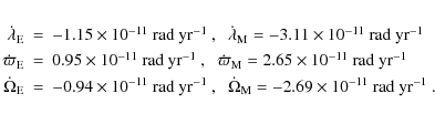
With the exception of the mean longitude of Mars, the observed drifts agree well with the analytical predictions of Table 2. For Mars, the discordance with the predicted drift in mean longitude is due to the non zero mean value of the perturbation of the semi-major axis of Mars. A constant shift in the semi-major axis corresponds to a shift in mean motion
We estimate the perturbation induced by the ring on the Earth-Mars distance by comparing two integrations with and without the ring. Figure 2 shows that with INPOP06 parameters the effect of the ring reaches approximately 150 m. This perturbation results from secular drifts in the various orbital elements, thus the 150 m reached over 31 years between 1969 and 2000 can be translated as approximately 5 m per year. This is in good agreement with the prediction made at the end of Sect. 2.3.
![\begin{figure}
\par\includegraphics[width=8cm,clip]{13346fg02.eps}
\end{figure}](/articles/aa/full_html/2010/06/aa13346-09/img84.png)
|
Figure 2: Perturbation of the Earth-Mars distance induced by a ring with INPOP06 parameters. |
| Open with DEXTER | |
4 A test model of the main belt
From the analytical standpoint the ring appears as a first-order representation of the main belt. Nevertheless, it is rather difficult to evaluate its effective capacity to model a multitude of objects. One possible solution is to test the ring against a test model containing large numbers of individual asteroids assigned with particular masses. The ring can be tested against many different asteroid models each built with a different set of masses. Such Monte Carlo (MC) experiments can provide an estimate of the number of asteroids that have to be modeled individually in ephemerides. If the asteroid masses are individually inaccurate but globally reasonable, the MC experiments can also estimate the ring's mass.
4.1 Asteroid selection
We select for our test model all the asteroids in the ASTORB catalog
that have an absolute magnitude brighter than 14 and are situated in
terms of semi-major axis within 3.5 AU. These
criteria are the same as in Sect. 2.1. The
absolute magnitude limit of 14 corresponds to the
estimated completeness limit of the main-belt and NEO populations as
reported by Jedicke
et al. (2002). The value also leads to a relatively
large but still reasonable number of objects to work with,
24635 asteroids in total. Absolute magnitude can be converted
to diameter with the following formula (Bowell
et al. 1989):
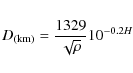
where D is the diameter in kilometers, H the absolute magnitude, and
4.2 Asteroid masses
Table 4: Albedo and corresponding uncertainty for objects with known taxonomy or belonging to a dynamical family.
Today the total number of accurately measured asteroid masses
amounts to only a few tens. Besides the case of binary objects,
asteroid mass determinations are in general susceptible to systematic
errors, which are hard to estimate. To assign all the selected
asteroids with at least reasonable masses, we devise a simple algorithm
inspired by the statistical asteroid model (Tedesco
et al. 2005). The algorithm processes family
membership, taxonomy, and SIMPS survey data![]() and assigns accordingly each asteroid with an albedo
and assigns accordingly each asteroid with an albedo ![]() and corresponding uncertainty
and corresponding uncertainty ![]() .
Among the 24635 asteroids, more than two thousand asteroids have values
of
.
Among the 24635 asteroids, more than two thousand asteroids have values
of ![]() and
and ![]() directly available from SIMPS, objects with family or taxonomy data
have their
directly available from SIMPS, objects with family or taxonomy data
have their ![]() and
and ![]() attributed with data obtained in the statistical asteroid model and
reproduced in Table 4.
In cases where information overlaps, SIMPS is preferred to taxonomies
and families. Taxonomy data is preferred to families, which helps to
eliminate interlopers in the family data. In general at least some
information is available for 10% of the selected objects. For the
remaining majority of asteroids, they are randomly assigned an albedo
class with probabilities adopted from Tedesco
et al. (2005) (56% low albedo, 7% intermediate
albedo, 34% moderate albedo, and 3% high albedo). Table 4 defines
attributed with data obtained in the statistical asteroid model and
reproduced in Table 4.
In cases where information overlaps, SIMPS is preferred to taxonomies
and families. Taxonomy data is preferred to families, which helps to
eliminate interlopers in the family data. In general at least some
information is available for 10% of the selected objects. For the
remaining majority of asteroids, they are randomly assigned an albedo
class with probabilities adopted from Tedesco
et al. (2005) (56% low albedo, 7% intermediate
albedo, 34% moderate albedo, and 3% high albedo). Table 4 defines ![]() and
and ![]() for each albedo class.
for each albedo class.
Asteroid diameters are calculated from corresponding ![]() to which a random error within
to which a random error within
![]() is
added. For SIMPS data, the algorithm ignores the formal
is
added. For SIMPS data, the algorithm ignores the formal
![]() and applies
instead a more realistic 10% uncertainty directly on the
diameter. As potential systematic errors in absolute magnitudes are
reported by various authors (Juric
et al. 2002), we account for them with a
and applies
instead a more realistic 10% uncertainty directly on the
diameter. As potential systematic errors in absolute magnitudes are
reported by various authors (Juric
et al. 2002), we account for them with a ![]() 0.5 random
uncertainty added to absolute magnitude. With the lower part of
Table 4,
we can use each asteroid's mean albedo
0.5 random
uncertainty added to absolute magnitude. With the lower part of
Table 4,
we can use each asteroid's mean albedo ![]() to assign the asteroid with a density class: C (low albedo), S
(moderate albedo), and M (intermediate and high albedos merged). We
stress that these density classes are attributed according to albedo.
Therefore, for some objects, the density classes may not coincide with
taxonomy data. Bulk porosity is expected to vary among the asteroids
(see Britt et al. 2002),
so we adopt the following intervals for the class densities: [0.5,2.5]
(C), [1.6,3.8] (S) and [1,5] (M). The density of an asteroid is chosen
randomly within the corresponding class interval and together with the
previously calculated diameter provides a mass. The masses of six
asteroids are kept constant and equal to their published values. We fix
to assign the asteroid with a density class: C (low albedo), S
(moderate albedo), and M (intermediate and high albedos merged). We
stress that these density classes are attributed according to albedo.
Therefore, for some objects, the density classes may not coincide with
taxonomy data. Bulk porosity is expected to vary among the asteroids
(see Britt et al. 2002),
so we adopt the following intervals for the class densities: [0.5,2.5]
(C), [1.6,3.8] (S) and [1,5] (M). The density of an asteroid is chosen
randomly within the corresponding class interval and together with the
previously calculated diameter provides a mass. The masses of six
asteroids are kept constant and equal to their published values. We fix
![]() ,
,
![]() ,
,
![]() for
1 Ceres, 2 Pallas, 4 Vesta (Fienga et al. 2008),
for
1 Ceres, 2 Pallas, 4 Vesta (Fienga et al. 2008),
![]() for
10 Hygiea (Chesley
et al. 2005),
for
10 Hygiea (Chesley
et al. 2005),
![]() for
22 Kalliope (Merline
et al. 1999), and
for
22 Kalliope (Merline
et al. 1999), and
![]() for
45 Eugenia (Margot
& Brown 2005).
for
45 Eugenia (Margot
& Brown 2005).
We used the algorithm to generate for each asteroid a set
of 100 random masses. A standard mass set is
generated without any random choices. In this standard mass set,
![]() is put to
zero and densities are maintained at INPOP06 values:
1.56 (C), 2.18 (S), and 4.26 (M).
Objects without any available data are automatically considered as
belonging to the C taxonomy class in the standard mass set.
is put to
zero and densities are maintained at INPOP06 values:
1.56 (C), 2.18 (S), and 4.26 (M).
Objects without any available data are automatically considered as
belonging to the C taxonomy class in the standard mass set.
4.3 Individual perturbations and the global effect
As in Sect. 3,
the perturbation of the Earth-Mars distance is denoted with ![]() .
To evaluate the perturbations
.
To evaluate the perturbations ![]() (
(
![]() )
induced by each individual asteroid of the test model, we performed
extensive integrations with INPOP. Each
)
induced by each individual asteroid of the test model, we performed
extensive integrations with INPOP. Each
![]() was obtained
by comparing on the 1969-2010 interval a Solar System
integration with the particular asteroid and a reference integration in
which the asteroid is absent.
was obtained
by comparing on the 1969-2010 interval a Solar System
integration with the particular asteroid and a reference integration in
which the asteroid is absent.
For a given set of asteroid masses, we can rank the asteroids
according to the decreasing amplitude of their individual
perturbations. Here and in the following, the amplitude of a
perturbation is estimated by the maximum of
![]() reached
on the 1969-2010 interval. Each
reached
on the 1969-2010 interval. Each
![]() is
proportional to the mass Mi
of the perturbing asteroid, in consequence, we have
is
proportional to the mass Mi
of the perturbing asteroid, in consequence, we have
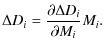
Equation (5) can be rewritten as

where D is the Earth-Mars distance. This is the analog of Eq. (4), but instead of considering the perturbation of the Earth-Mars distance as depending on the perturbations of the planetary orbits, we consider it as depending on the mass of the perturbing asteroid. The first-order Taylor expansion of D in terms of all the asteroid masses leads to
We can thus approximate to first-order the perturbation caused by a particular set of asteroid masses by the sum of the already calculated individual asteroid contributions:
Although initially the
To test the development (6), we can compare the global perturbation obtained from a simultaneous INPOP integration of all the asteroids, but the N most perturbing ones with the same perturbation obtained from the development. We choose N at 300 here because it corresponds to the number of asteroids usually considered individually in modern ephemerides. Figure 3 shows the difference between the two perturbations for the standard mass set. This difference is on the order of 1 m, which is less than 1% of the perturbation's amplitude. In consequence, we consider the development (6) as satisfactory. It should be noted, that in the simultaneous integration, the mutual perturbations of the asteroids were not taken into account.
![\begin{figure}
\par\includegraphics[width=8.5cm,clip]{13346fg03.eps}
\end{figure}](/articles/aa/full_html/2010/06/aa13346-09/img103.png)
|
Figure 3:
Difference between the |
| Open with DEXTER | |
5 Testing the capacity of the ring to model large numbers of asteroids
5.1 Selection based on amplitude
![\begin{figure}
\par\includegraphics[width=8.5cm,clip]{13346fg04.eps}
\end{figure}](/articles/aa/full_html/2010/06/aa13346-09/img104.png)
|
Figure 4: Evolution of R(N) for the standard set of masses (in gray) and an average over 100 different sets. |
| Open with DEXTER | |
We denote with ![]() the global perturbation induced on the Earth-Mars distance by the test
model after removing from the test model the N most
perturbing asteroids. Similarly we denote with
the global perturbation induced on the Earth-Mars distance by the test
model after removing from the test model the N most
perturbing asteroids. Similarly we denote with
![]() the
perturbation induced by a ring. To evaluate the capacity of the
ring to represent the global perturbation, we fit for different values
of N the amplitude of
the
perturbation induced by a ring. To evaluate the capacity of the
ring to represent the global perturbation, we fit for different values
of N the amplitude of
![]() so
as to minimize
so
as to minimize
Because
Figure 4 shows the evolution of R(N) for the standard set of masses, as well as an average of R(N) over the 100 different mass sets defined in Sect. 4.2. For values of N greater than 200, the ability of the ring to model a global effect has reached its maximum and remains constant. At its best, the ring is thus able to represent more than 80
We show in Fig. 5 the effect induced on the planetary orbital elements by the test model after removing from the test model the 300 most perturbing asteroids (for the standard mass set). The observed effects are indeed rather smooth and similar to the drifts induced by a ring. For comparison, Fig. 6 shows the effect induced on the planetary orbital elements by all the asteroids of the test model.
![\begin{figure}
\par\includegraphics[width=8.4cm,clip]{13346fg05.eps}
\end{figure}](/articles/aa/full_html/2010/06/aa13346-09/img110.png)
|
Figure 5: Perturbation induced on the orbital elements of Earth (in gray) and Mars by the test model after removing from the test model the 300 most important perturbers. |
| Open with DEXTER | |
![\begin{figure}
\par\includegraphics[width=8.7cm,clip]{13346fg06.eps}
\end{figure}](/articles/aa/full_html/2010/06/aa13346-09/img111.png)
|
Figure 6: Perturbation induced on the orbital elements of Earth (in gray) and Mars by the entire test model. |
| Open with DEXTER | |
![\begin{figure}
\par\includegraphics[width=8.5cm,clip]{13346fg07.eps}
\end{figure}](/articles/aa/full_html/2010/06/aa13346-09/img112.png)
|
Figure 7:
Evolution of the amplitude of
|
| Open with DEXTER | |
It is possible to calculate the average mass of the ring after removing
the 300 most perturbing asteroids by minimizing
With the 100 different sets of asteroid masses, the mass of the ring is estimated at
The calculated residuals for N = 300 correspond to approximately 10 m over the 2000-2010 time interval. This is an order of magnitude above the residuals obtained today for the most accurate Mars ranging data. The limiting factor of the ring model is the inability to reproduce the quadratic evolution in the mean longitude of Mars (see Fig. 5). This quadratic evolution is in fact a consequence of the linear drift of the semi-major axis of Mars that persists in the test model for all values of N.
5.2 The selection as a mixed integer quadratic problem
The progressive removal of asteroids from the test model can be understood as a selection of individual asteroids that should be modeled individually in an ephemeris. The selection scheme based on the amplitude of the individual asteroid perturbations on the Earth-Mars distance is not optimal. Indeed for each state N, it is possible to slightly modify the set of the removed asteroids in order to eliminate the linear drift in the semi-major axis of Mars responsible for the quadratic evolution of the mean longitude in Fig. 5. The modification consists of removing from the test model a few additional asteroids that induce a positive slope in the perturbation of the semi-major axis of Mars and adding the same number of already removed objects with a negative slope. Such changes improve the average residuals from the previous 38 m to 20 m.
A more systematic approach is to use a combinatorial
optimization algorithm to select among the N most
perturbing asteroids those that should be removed from the test model
in order to maximize the modeling capacity of the ring. The problem can
be stated formally for a particular mass set and a given N
as the search for N+1 parameters ![]() that minimize
that minimize
with the constraint that
Figure 8
gives the analog of R(N)
obtained with a new selection scheme using the MIQP formulation, we
denote the global effect corresponding to this new scheme with
![]() .
Because the calculations are relatively time consuming, only values
of N below 500 are considered. For
each N the algorithm uses CPLEX to select
among the N most perturbing asteroids,
those that should be removed from the test model to obtain an optimal
fit with a ring. For N greater
than 200, only the 200 least perturbing asteroids
among the N most perturbing ones are considered by
CPLEX. The remaining (N-200) are removed from the
test model automatically. In Fig. 8 we observe that
the ring's modeling capacity is greatly improved when compared with the
selection scheme based on amplitude. Not only does R(N)
drop almost to zero, but the maximum modeling capacity is also reached
earlier. Figure 9
shows the evolution of the average maximum reached by the global
perturbation and of the corresponding residuals after fitting the ring.
Although the amplitude of the global effect is almost twice as large as
in Fig. 7,
the residuals are greatly improved. The performance reached after
removing the 300 most perturbing asteroids from the test model is
obtained with the MIQP approach for N = 50. The
average residuals after fitting the ring are 4 m for N
= 300. This corresponds to approximately 1.3 m over
10 years. The unmodeled part of the global perturbation is
thus below the one sigma residuals of the MGS/MO and MEX data obtained
in INPOP08. The average maximum reached by the global effect is
472 m, which corresponds in terms of the ring's mass to
.
Because the calculations are relatively time consuming, only values
of N below 500 are considered. For
each N the algorithm uses CPLEX to select
among the N most perturbing asteroids,
those that should be removed from the test model to obtain an optimal
fit with a ring. For N greater
than 200, only the 200 least perturbing asteroids
among the N most perturbing ones are considered by
CPLEX. The remaining (N-200) are removed from the
test model automatically. In Fig. 8 we observe that
the ring's modeling capacity is greatly improved when compared with the
selection scheme based on amplitude. Not only does R(N)
drop almost to zero, but the maximum modeling capacity is also reached
earlier. Figure 9
shows the evolution of the average maximum reached by the global
perturbation and of the corresponding residuals after fitting the ring.
Although the amplitude of the global effect is almost twice as large as
in Fig. 7,
the residuals are greatly improved. The performance reached after
removing the 300 most perturbing asteroids from the test model is
obtained with the MIQP approach for N = 50. The
average residuals after fitting the ring are 4 m for N
= 300. This corresponds to approximately 1.3 m over
10 years. The unmodeled part of the global perturbation is
thus below the one sigma residuals of the MGS/MO and MEX data obtained
in INPOP08. The average maximum reached by the global effect is
472 m, which corresponds in terms of the ring's mass to
![]() .
.
We show in Fig. 10, the perturbation induced on the orbital elements of Earth and Mars by the global effect obtained with the MIQP selection (N = 300) and the standard set of asteroid masses. The quadratic evolution of the mean longitude of Mars from Fig. 5 is straightened up. This explains why the corresponding global effect on the Earth-Mars distance has increased in amplitude. The MIQP approach in general improves the resemblance between the effect on the orbital elements induced by the global perturbation and the ring. A comparison between Figs. 1, 5, and 10 shows that beside improvements in the semi-major axis and mean longitude perturbations, the new selection also improves the eccentricity and perihelion perturbations. There are still some discrepancies, most importantly in the perturbations induced on the inclinations and nodes as well as on the perihelium of the Earth; however, these discrepancies are not surprising as the asteroid selection is based only on the Earth-Mars distance, which according to Table 3 is not very sensitive to these parameters.
![\begin{figure}
\par\includegraphics[width=8.5cm,clip]{13346fg08.eps}
\end{figure}](/articles/aa/full_html/2010/06/aa13346-09/img121.png)
|
Figure 8: Evolution of R(N) with the MIQP selection for the standard set of masses (in gray) and an average over 100 different sets. The dashed line represents the average R(N) obtained with the selection based on amplitude. |
| Open with DEXTER | |
![\begin{figure}
\par\includegraphics[width=8.5cm,clip]{13346fg09.eps}
\end{figure}](/articles/aa/full_html/2010/06/aa13346-09/img122.png)
|
Figure 9:
Evolution with the MIQP selection of the amplitude of
|
| Open with DEXTER | |
![\begin{figure}
\par\includegraphics[width=8.8cm,clip]{13346fg10.eps}
\end{figure}](/articles/aa/full_html/2010/06/aa13346-09/img123.png)
|
Figure 10: Perturbation induced on the orbital elements of Earth (in gray) and Mars by the test model after removing from the test model at most 300 asteroids with the MIQP selection. |
| Open with DEXTER | |
5.3 Accounting for all the inner planets
Today ephemerides are being fitted to accurate Venus ranging observations from the ongoing VEX mission (see Fienga et al. 2009). According to Ashby et al. (2007), Mercury ranging could become available within a few years with missions like Messenger or BepiColombo. To evaluate the ability of the ring to model the global effect on all the inner planets, we repeated the MC experiment made with the MIQP selection scheme in Sect. 5.2. Instead of fitting only the Earth-Mars distance, we simultaneously fit the effects on distances to Mercury, Venus, and Mars. Figure 11 shows the evolution of residuals for all the planets in the simultaneous fit. For comparison the figure shows the residuals that can be obtained by fitting the distance to each planet separately. For N = 300, the ring is able to represent the global effect simultaneously on all the inner planets with an average accuracy better than 1.6 m over a 10 years time interval. Fitting all the planets together for N = 300 leads to the same amplitude of the global perturbation as in Sect. 5.2, and hence to the same estimate of the ring's mass. When considering separately Mercury or Venus, Fig. 11 shows that residuals well below 1 m per year can be reached by removing merely 1 Ceres, 2 Pallas and 4 Vesta from the main belt.
![\begin{figure}
\par\includegraphics[width=8.8cm,clip]{13346fg11.eps}
\end{figure}](/articles/aa/full_html/2010/06/aa13346-09/img124.png)
|
Figure 11:
Average residuals computed with the MIQP selection
over 100 random mass sets for the Earth-Mars (a
and a'), Earth-Venus (b and b'), and
Earth-Mercury distances (c and c'). The continuous lines
represent residuals obtained from a simultaneous fit of the ring to the
|
| Open with DEXTER | |
Table 5: Asteroids with an effect on the Earth-Mars distance greater than 100 m.
6 Applications
6.1 Model selection
To model the global effect correctly with respect to the accuracy of
available data, a reasonable choice according to Fig. 11 is to
account for fewer than 300 individual objects. By examining asteroids
that were removed from the test model during the MC experiments, we can
compile a list of objects that should be modeled individually in an
ephemeris. For N = 300 in the simultaneous fit of
Sect. 5.3,
a total of 523 asteroids were removed at least once from the test model
during the 100 MC runs, and the average number of
removed objects was approximately 240. In an ephemeris with an
idealized asteroid model we should therefore fit these
523 asteroid masses with the option of putting more than a
half of the fitted values to zero. Among the 523 asteroids,
there are 72 individuals removed from the test model on each
run and 60 asteroids removed only once during the
100 runs. The distinction between asteroids having a high
chance of removal and a low one is not clear, it is however possible to
define an arbitrary limit above which the probability of being removed
from the test model is reasonably high. Fixing this limit at ![]() leads to a total of 287 objects, which are listed in
Table A.1 of the supplementary online material. The table
provides for each asteroid the probability of being selected as well as
its maximum effects on the Earth-Mars, Earth-Venus, and Earth-Mercury
distances during the 1969-2010 time interval (for the standard
mass set). It is interesting to note the existence of asteroids with
relatively small effects on the Earth-Mars distance but with very high
probabilities of being included in the individual part of the asteroid
model: for example, 758 Mancunia induces a perturbation of
approximately 10 m, but it is removed on each of the
100 runs. A part of Table A.1 of the supplementary
online material is reproduced in Table 5.
leads to a total of 287 objects, which are listed in
Table A.1 of the supplementary online material. The table
provides for each asteroid the probability of being selected as well as
its maximum effects on the Earth-Mars, Earth-Venus, and Earth-Mercury
distances during the 1969-2010 time interval (for the standard
mass set). It is interesting to note the existence of asteroids with
relatively small effects on the Earth-Mars distance but with very high
probabilities of being included in the individual part of the asteroid
model: for example, 758 Mancunia induces a perturbation of
approximately 10 m, but it is removed on each of the
100 runs. A part of Table A.1 of the supplementary
online material is reproduced in Table 5.
6.2 Systematic error estimation
It is possible to use the results obtained in Fig. 11 to estimate systematic errors that will be induced by the residuals of the global perturbation during future missions like BepiColombo. These systematic errors can have a significant impact on the planned determinations of physical parameters from the ranging data. An extensive study of this problem is presented in Ashby et al. (2007).
The BepiColombo mission is expected to generate ranging data to Mercury accurate down to 4.5 cm (see Ashby et al. 2007). Figure 11 shows that 4.5 cm per year is relatively close to the best possible residuals reached for the Earth-Mercury distance. To take full advantage of this accuracy, the asteroid model used to process the ranging data will have to correctly account for approximately 200 individual asteroids. This is a relatively high number because obtaining accurate estimates of 200 asteroid masses may still be difficult in the near future. If we estimate at 50 the number of asteroids that we are actually able to model with the highest accuracy, we can use Fig. 11 to obtain an estimate of the systematic error for the BepiColombo mission if it took place today. For N = 50, fitting only the Earth-Mercury distance leads to residuals of approximately 6 m equivalent to a systematic error of 15 cm over a one year period.
7 Discussion
It was shown that with an appropriate selection scheme a ring is able
to effectively reduce the amplitude of a perturbation induced by
thousands of asteroids from an average 472 m to
only 4 m. The ring thus represents more than 99![]() of the global perturbation, which clearly makes it a very suitable
model. The value of 99
of the global perturbation, which clearly makes it a very suitable
model. The value of 99![]() was obtained with 100 MC experiments, so it can be
considered as quite robust. Also, this percentage does not depend on
choices made for attributing asteroids with masses in the test model.
The estimations of the amplitude of the residuals, the amplitude of the
global perturbation and the mass of the ring are, on the other hand,
proportional to the mass of the test model and in consequence strongly
dependent on the choices made in the attribution of asteroid masses. If
for example in Sect. 4.2 the
interval used for the C density class were centered
on 1 instead of 1.5, all the previous
parameters would have been approximately one third smaller. We are
reasonably confident in the realism of the asteroid masses in our model
because the mass of the ring obtained after removing the
300 most perturbing asteroids in Sect. 5.1 is relatively
close to the value of
was obtained with 100 MC experiments, so it can be
considered as quite robust. Also, this percentage does not depend on
choices made for attributing asteroids with masses in the test model.
The estimations of the amplitude of the residuals, the amplitude of the
global perturbation and the mass of the ring are, on the other hand,
proportional to the mass of the test model and in consequence strongly
dependent on the choices made in the attribution of asteroid masses. If
for example in Sect. 4.2 the
interval used for the C density class were centered
on 1 instead of 1.5, all the previous
parameters would have been approximately one third smaller. We are
reasonably confident in the realism of the asteroid masses in our model
because the mass of the ring obtained after removing the
300 most perturbing asteroids in Sect. 5.1 is relatively
close to the value of
![]() obtained in
INPOP06.
obtained in
INPOP06.
The objective in this work was to show that the ring is a
first-order model of a main-belt global effect and that it is able to
represent large numbers of objects in practice. The difficulty of
fitting its mass with other highly correlated parameters is an
important problem not considered here. In particular, the initial
conditions of the planets were maintained fixed throughout our study,
whereas they are fitted in an ephemeris. Because the global effect acts
mostly through linear drifts in mean-longitudes, a large part can be
absorbed by changes of a few meters in the initial semi-major axes of
the planets. The mass of the ring can be correlated with other
parameters as well, like the individual asteroid masses or for example
solar oblateness as shown by Fienga
et al. (2009). These correlations can be considered
as so important that the ring is eventually not implemented in the
model (the case in DE421) or its mass is fixed to a certain value (the
case for INPOP08). The major arguments for keeping the ring in the
model are its 99![]() modeling capacity and that, without the ring, systematic errors can
reach several hundreds of meters.
modeling capacity and that, without the ring, systematic errors can
reach several hundreds of meters.
In Sect. 2.1 we fixed the radius of the ring to 2.8 AU and always considered mass as the only parameter. We have briefly investigated the possibility of fitting the radius and mass together. We find out that, when considering only the Earth-Mars distance, any change in mass can effectively be compensated for by a change in radius. In terms of the residuals on the Earth-Mars distance, moving the ring from 2.8 AU to 2.4 AU is equivalent to doubling the ring's mass. Similarly moving the ring to 3.4 AU is equivalent to dividing the mass of the ring by two. The same residuals can be obtained no matter the radius. Nevertheless according to Sect. 2.1, the mass of a ring with radius 2.8 AU indeed corresponds to the total mass of the represented asteroids (it is not the case for other radii).
Throughout this paper, we estimated the amplitudes of
perturbations with the maximum reached on the 1969-2010 interval. This
corresponds to the maximum norm
![]() .
Measuring perturbations in terms of the root mean square (equivalent to
the norm
.
Measuring perturbations in terms of the root mean square (equivalent to
the norm ![]() )
would divide all our amplitude estimations by approximately three. This
would lead to much more relaxed demands on the asteroid models. In
particular an accuracy below 2 m over 10 years would
be reached in Fig. 11
for N = 100 instead of N = 300.
Similarly, the final systematic error for BepiColombo with a correct N=50
asteroid model would drop from 15 cm per year
to 5 cm per year. We showed that the number of
asteroids that need to be accounted for individually is no more
than 300, if in a more optimistic perspective all our
amplitude estimations can be divided by a factor of three, the number
of asteroids to account for individually could be as low
as 100.
)
would divide all our amplitude estimations by approximately three. This
would lead to much more relaxed demands on the asteroid models. In
particular an accuracy below 2 m over 10 years would
be reached in Fig. 11
for N = 100 instead of N = 300.
Similarly, the final systematic error for BepiColombo with a correct N=50
asteroid model would drop from 15 cm per year
to 5 cm per year. We showed that the number of
asteroids that need to be accounted for individually is no more
than 300, if in a more optimistic perspective all our
amplitude estimations can be divided by a factor of three, the number
of asteroids to account for individually could be as low
as 100.
This study was restricted to the main-belt perturbations. Other Solar System objects potentially have impacts on the ephemerides that should be estimated and possibly accounted for. We can mention trans-Neptunian objects already implemented in the EPM ephemeris or the Trojan asteroids whose effect could be significant and which are certainly not accounted for by a ring. Also we only considered effects on the inner planets because they provide the majority of accurate data today. The effect of asteroids on the outer planets can be non-negligible and should be considered in future studies; especially, effects on Jupiter can be significant because of the various resonances with the main belt. However, such studies for the outer planets will have an impact on data only when accurate observations of the outer planets are available over a sufficient time span.
8 Conclusion
A ring is an implementation of an averaged orbit, which is a very good
model of the perturbation induced by the main-belt asteroids. After
removing less than 300 objects from the main-belt, the ring is
able to account for more than 99![]() of the remaining perturbation on all the inner planets. Since the
amplitude of the global effect can reach several hundreds of meters in
terms of the Earth-Mars distance, it is advisable to keep the ring in
an ephemeris model of the Solar System.
of the remaining perturbation on all the inner planets. Since the
amplitude of the global effect can reach several hundreds of meters in
terms of the Earth-Mars distance, it is advisable to keep the ring in
an ephemeris model of the Solar System.
Appendix A: 3D perturbing force of an asteroid ring
![\begin{figure}
\par\includegraphics[width=8.5cm,clip]{13346fg12.eps}
\end{figure}](/articles/aa/full_html/2010/06/aa13346-09/img128.png)
|
Figure A.1: The reference frame. |
| Open with DEXTER | |
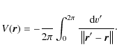
We derive here the expression of the gravitational force
exerted by a ring of center O, radius r',
and mass m on a point P of
mass M. The chosen reference frame is
![]() ,
with
,
with ![]() orthogonal to the ring's plane and
orthogonal to the ring's plane and ![]() the unit vector in the direction of the projection of
the unit vector in the direction of the projection of
![]() on
the ring's plane. We denote with
on
the ring's plane. We denote with ![]() the radius vector of a point on the ring. The longitude angle of
the radius vector of a point on the ring. The longitude angle of ![]() with origin at
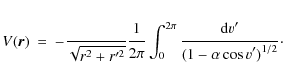
with origin at ![]() is denoted v' (see Fig. A.1). The potential
exerted by the ring on P is
is denoted v' (see Fig. A.1). The potential
exerted by the ring on P is
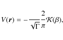
By defining I as the angle of
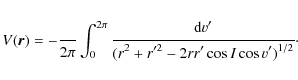
With
we obtain
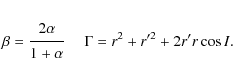
The above expression can be rewritten as
where
The force exerted on P is
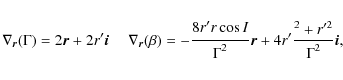
we obtain, after straightforward computation, the expression of
![\begin{eqnarray*}\vec{F} = -{{\displaystyle\strut2 GmM}\over{\displaystyle\strut...
...\alpha){\cal K}(\beta) -{\cal E}(\beta)\right) r'{\vec i}\Big] .
\end{eqnarray*}](/articles/aa/full_html/2010/06/aa13346-09/img150.png)
This expression is valid for an internal or external body P with
The first author wishes to acknowledge interesting discussions with James Hilton (US Naval Observatory). This work was done with the financial support of the CNES and the French Ministry of Education.
References
- Ashby, N., Bender, P. L., & Wahr, J. M. 2007, Phys. Rev. D, 75
- Bowell, E., Hapke, B., Lumme, K., & Harris, A. W. 1989, in Asteroids II (Univ. Arizona Press), 549
- Britt, D. T., Yeomans, D., Housen, K., & Consolmagno, G. 2002, in Asteroids III (Univ. Arizona Press), 485
- Chesley, S. R., Owen, W. M., Hayne, E. W., et al. 2005, Bull. Am. Astron. Soc., 37, 524
- Fienga, A., Manche, H., Laskar, J., & Gastineau, M. 2008, A&A, 477, 315
- Fienga, A., Laskar, J., Manche, H., et al. 2009, Relativity in Fundamental Astronomy: Dynamics, Reference Frames and Data analysis, Proc. IAU Symp., 261
- Fienga, A., Laskar, J., Morley, T., et al. 2009, A&A, 507, 1675
- Folkner, W. M., Williams, J. G., & Boggs, D. H. 2008, JPL IOM 343R-08-003
- Gueye, S., & Michelon, P. 2009, Discrete Applied Mathematics, 157
- Hill, G. W. 1882, Astronomical papers prepared for the use of the American Ephemeris, I
- Jedicke, R., Larsen, J., & Spahr, T. 2002, in Asteroids III (Univ. Arizona Press), 98
- Juric, M., Ivezic, Z., Lupton, R. H., et al. 2002, AJ, 124, 1776
- Krasinsky, G. A., Pitjeva, E. V., Vasilyev, M. V., & Yagudina, E. I. 2002, Icarus, 158, 98
- Laskar, J., & Robutel, P. 1995, Celestial Mechanics and Dynamical Astronomy, 62, 193
- Margot, J. L., & Brown, M. E. 2005, Science, 300, 1939
- Merline, W. J., Close, L. M., Dumas, C., et al. 1999, Nature, 401, 565
- Murray, C. D., & Dermott, S. F. 1999, in Solar System dynamics (Cambridge University Press), 225
- Tedesco, E. F., Cellino, A., & Zappala, V. 2005, AJ, 129, 2869
- Whittaker, E. T., & Watson, G. N. 1927, in A course of Modern Analysis (Cambridge University Press)
Online Material
Table A.1:
Asteroids selected for the individual part of the asteroid model when
simultaneously fitting ranging data on all four inner planets. As
described in Sect. 6,
only asteroids with probability greater than ![]() of being removed from the test model during the 100 MC experiments are
listed. For each asteroid this probabilty is given together with the
asteroid's diameter, density class (in the standard mass set) and
correponding perturbations on the Earth-Mars, Earth-Venus, and
Earth-Mercury distances in terms of max
of being removed from the test model during the 100 MC experiments are
listed. For each asteroid this probabilty is given together with the
asteroid's diameter, density class (in the standard mass set) and
correponding perturbations on the Earth-Mars, Earth-Venus, and
Earth-Mercury distances in terms of max
![]() on
the 1969-2010 time interval. Density classes are assigned according
to albedo (see Sect. 4.2) and do
not always correspond to taxonomies.
on
the 1969-2010 time interval. Density classes are assigned according
to albedo (see Sect. 4.2) and do
not always correspond to taxonomies.
Footnotes
- ... ephemerides
- Table A.1 is only available in electronic form at http://www.aanda.org
- ... ASTORB
- The asteroid orbits are calculated for the 27 October 2007.
- ... data
- The databases are maintained in NASA's PDS Asteroid Archive.
- ... CPLEX
- The software solves a hierarchy of linear subproblems in a branch-and-bound approach, see www.ilog.com/products/cplex for more details on the package.
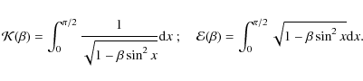
- ... integral
- The elliptical integral of first (
 )
and second (
)
and second ( )
kind are defined as (Whittaker
& Watson 1927):
)
kind are defined as (Whittaker
& Watson 1927):
All Tables
Table 1: Parameters of an averaged orbit representing the main-belt perturbation as determined from the perturbation on the inner planets.
Table 2: Secular effect of a ring, with INPOP06 parameters, on the orbital elements of the Earth and Mars.
Table 3: The Earth-Mars distance dependence on the orbital elements.
Table 4: Albedo and corresponding uncertainty for objects with known taxonomy or belonging to a dynamical family.
Table 5: Asteroids with an effect on the Earth-Mars distance greater than 100 m.
Table A.1:
Asteroids selected for the individual part of the asteroid model when
simultaneously fitting ranging data on all four inner planets. As
described in Sect. 6,
only asteroids with probability greater than ![]() of being removed from the test model during the 100 MC experiments are
listed. For each asteroid this probabilty is given together with the
asteroid's diameter, density class (in the standard mass set) and
correponding perturbations on the Earth-Mars, Earth-Venus, and
Earth-Mercury distances in terms of max
of being removed from the test model during the 100 MC experiments are
listed. For each asteroid this probabilty is given together with the
asteroid's diameter, density class (in the standard mass set) and
correponding perturbations on the Earth-Mars, Earth-Venus, and
Earth-Mercury distances in terms of max
![]() on
the 1969-2010 time interval. Density classes are assigned according
to albedo (see Sect. 4.2) and do
not always correspond to taxonomies.
on
the 1969-2010 time interval. Density classes are assigned according
to albedo (see Sect. 4.2) and do
not always correspond to taxonomies.
All Figures
|
|
Figure 1: Perturbation induced on the orbital elements of Earth (in gray) and Mars by a ring with INPOP06 parameters. |
| Open with DEXTER | |
| In the text | |
|
|
Figure 2: Perturbation of the Earth-Mars distance induced by a ring with INPOP06 parameters. |
| Open with DEXTER | |
| In the text | |
|
|
Figure 3:
Difference between the |
| Open with DEXTER | |
| In the text | |
|
|
Figure 4: Evolution of R(N) for the standard set of masses (in gray) and an average over 100 different sets. |
| Open with DEXTER | |
| In the text | |
|
|
Figure 5: Perturbation induced on the orbital elements of Earth (in gray) and Mars by the test model after removing from the test model the 300 most important perturbers. |
| Open with DEXTER | |
| In the text | |
|
|
Figure 6: Perturbation induced on the orbital elements of Earth (in gray) and Mars by the entire test model. |
| Open with DEXTER | |
| In the text | |
|
|
Figure 7:
Evolution of the amplitude of
|
| Open with DEXTER | |
| In the text | |
|
|
Figure 8: Evolution of R(N) with the MIQP selection for the standard set of masses (in gray) and an average over 100 different sets. The dashed line represents the average R(N) obtained with the selection based on amplitude. |
| Open with DEXTER | |
| In the text | |
|
|
Figure 9:
Evolution with the MIQP selection of the amplitude of
|
| Open with DEXTER | |
| In the text | |
|
|
Figure 10: Perturbation induced on the orbital elements of Earth (in gray) and Mars by the test model after removing from the test model at most 300 asteroids with the MIQP selection. |
| Open with DEXTER | |
| In the text | |
|
|
Figure 11:
Average residuals computed with the MIQP selection
over 100 random mass sets for the Earth-Mars (a
and a'), Earth-Venus (b and b'), and
Earth-Mercury distances (c and c'). The continuous lines
represent residuals obtained from a simultaneous fit of the ring to the
|
| Open with DEXTER | |
| In the text | |
|
|
Figure A.1: The reference frame. |
| Open with DEXTER | |
| In the text | |
Copyright ESO 2010
Current usage metrics show cumulative count of Article Views (full-text article views including HTML views, PDF and ePub downloads, according to the available data) and Abstracts Views on Vision4Press platform.
Data correspond to usage on the plateform after 2015. The current usage metrics is available 48-96 hours after online publication and is updated daily on week days.
Initial download of the metrics may take a while.