Photometric redshifts for type Ia supernovae in the supernova legacy survey

N. Palanque-Delabrouille; V. Ruhlmann-Kleider; S. Pascal; J. Rich; J. Guy; G. Bazin; P. Astier; C. Balland; S. Basa; R. G. Carlberg; A. Conley; D. Fouchez; D. Hardin; I. M. Hook; D. A. Howell; R. Pain; K. Perrett; C. J. Pritchet; N. Regnault; M. Sullivan

doi:10.1051/0004-6361/200913283

Free Access

Issue		A&A Volume 514, May 2010


Article Number		A63
Number of page(s)		7
Section		Cosmology (including clusters of galaxies)
DOI		https://doi.org/10.1051/0004-6361/200913283
Published online		20 May 2010

A&A 514, A63 (2010)

Photometric redshifts for type Ia supernovae in the supernova legacy survey

N. Palanque-Delabrouille¹ - V. Ruhlmann-Kleider¹ - S. Pascal¹ - J. Rich¹ - J. Guy² - G. Bazin¹ - P. Astier² - C. Balland^2,3 - S. Basa⁴ - R. G. Carlberg⁶ - A. Conley¹⁰ - D. Fouchez⁷ - D. Hardin² - I. M. Hook^9,11 - D. A. Howell^12,13 - R. Pain² - K. Perrett⁶ - C. J. Pritchet⁸ - N. Regnault² - M. Sullivan⁹

1 - CEA, Centre de Saclay, Irfu/SPP, 91191 Gif-sur-Yvette, France
2 - LPNHE, Université Pierre et Marie Curie, Université Paris diderot, CNRS-IN2P3, 4 place Jussieu, 75252 Paris Cedex 05, France
3 - University Paris 11, 91405 Orsay, France
4 - LAM, CNRS, BP8, Pôle de l'étoile, Site de Château-Gombert, 38 rue Frédéric Joliot-Curie, 13388 Marseille Cedex 13, France
5 - LUTH, UMR 8102 CNRS, Observatoire de Paris, Section de Meudon, 92195 Meudon Cedex, France
6 - Deparment of Astronomy and Astrophysics, University of Toronto, 50 St. George Street, Toronto, ON M5S 3H8, Canada
7 - CPPM, CNRS-Luminy, Case 907, 13288 Marseille Cedex 9, France
8 - Department of Physics and Astronomy, University of Victoria, PO Box 3055, Victoria, BC V8W 3P6, Canada
9 - Department of Physics (Astrophysics), University of Oxford, Denys Wilkinson Building, Keble Road, Oxford OX1 3RH, UK
10 - Center for Astrophysics and Space Astronomy, University of Colorado, Boulder, CO 80309-0389, USA
11 - INAF - Osservatorio Astronomico di Roma, via Frascati 33, 00040 Monteporzio (RM), Italy
12 - Las Cumbres Observatory Global Telescope Network, 6740 Cortona Dr., Suite 102, Goleta, CA 93117, USA
13 - Department of Physics, University of California, Santa Barbara, Broida Hall, Mail Code 9530, Santa Barbara, CA 93106-9530, USA

Received 11 September 2009 / Accepted 15 February 2010

Abstract
We present a method using the SALT2 light curve fitter to determine the redshift of type Ia supernovae in the Supernova Legacy Survey (SNLS) based on their photometry in g', r', i' and z'. On 289 supernovae of the first three years of SNLS data, we obtain a precision $\sigma_{\Delta z/(1+z)} = 0.022$ on average up to a redshift of 1.0, with a higher precision of 0.016 for z<0.45 and a lower one of 0.025 for z>0.45. The rate of events with $\vert\Delta z\vert/(1+z)>0.15$ (catastrophic errors) is 1.4%, and reduces to 0.4% when restricting the test sample of spectroscopically confirmed Type Ia supernovae. Both the precision and the rate of catastrophic errors are better than what can be currently obtained using host galaxy photometric redshifts. Photometric redshifts of this precision may be useful for future experiments which aim to discover up to millions of supernovae Ia but without spectroscopy for most of them.

Key words: cosmology: observations - methods: data analysis - stars: supernovae: general - surveys

1 Introduction

Ten years after the discovery of the accelerating expansion of the Universe, type Ia supernovae (SNe Ia) are still among the most accurate probes of dark energy. To study systematic effects more precisely, future experiments aim at an increase of several orders of magnitudes in the number of detected supernovae. Pan-STARRS Medium Deep Survey (MDS) and the Dark Energy Survey will discover thousands of supernovae up to a redshift of 1, though they will only be able to observe spectroscopically a fraction of them. The Large Synoptic Survey Telescope will discover roughly 250 000 type Ia SNe per year in the same redshift range, but again with only partial spectroscopic coverage (see the white paper of Howell et al. 2009, for a review of future surveys). While current surveys as the Supernova Legacy Survey (Astier et al. 2006) are already limited by the time available for spectroscopy, most future surveys will indeed have to count on an alternative to select the SNe Ia and determine their redshift from light curves only.

Studies solely based on photometry present the advantage of leading to larger sets of supernovae, that can be used to compare properties of SNe Ia in various subsamples, sorted for instance by redshift, SN color, or host morphology. The possibility to use solely photometric redshifts to derive cosmological constraints from SNe Ia, however, remains to be shown.

This paper addresses the question of obtaining photometric redshifts for SNe Ia. It presents a method that can be applied to ongoing as well as to future projects. The combination of a photometric selection of supernovae in the SNLS data, which doubles the number of supernovae compared to the real-time selection, with the photometric redshifts derived according to the method presented in this paper, will be the subject of a forthcoming study.

Previous works have already tackled the topic of SN Ia photometric redshifts. An empirical photometric redshift estimate for SNe Ia was proposed by Wang et al. (2007) who obtained a rms dispersion of 0.050 for 20 supernovae from the SNLS first year data not contained in the training set, and 0.031 for 20 supernovae used in the training. A method was also developed in SNLS for the needs of the real-time selection of SN Ia candidates to send for spectroscopy (Sullivan et al. 2006). It used the rising part of the light curves and a cosmology prior to both select tentative SN Ia candidates and derive an estimate of their redshift. Fits to the pre-maximum light data reached a precision $\sigma_{\vert\Delta z\vert/(1+z)} = 0.046$ while fits to the entire light curve a precision of 0.037.

The method presented in this paper aims at an improved precision on the photometric redshift, while remaining independent of the underlying cosmology. The study was calibrated with simulated SN Ia light curves, whose characteristics are given in Sect. 2. The method is presented in Sect. 3. To test its performance, it was applied to a large sample of SNe Ia from the first three years of SNLS data, presented in Sect. 2. The results obtained on this test sample are given in Sect. 4. A discussion on the method and on the impact of the underlying cosmology is presented in Sect. 5. The possible redsfhift biases and the precision of the method for various sub-classes of SNe Ia is discussed in Sect. 6. Conclusions are then given in Sect. 7.

2 SNLS data and simulation description

The SNLS data cover the redshift range between 0 and 1.2. They consist of four-band light curves obtained in a rolling search mode, leading to roughly 30 points per observing season in r' and i', 20 points in g' and 15 points in z'. The test sample used to quantify the perfomance of the method consists of a total of 289 SNe Ia passing color and stretch cuts (|c|<0.4, |x₁| < 4) to avoid events with extreme values compared to typical SNe Ia. It originates from the union of two sources: 241 are real-time selected events confirmed as ``Ia'' or ``Ia?'' by spectroscopy (Ellis et al. 2008; Balland et al. 2009; Bronder et al. 2008; Howell 2005), and the additional 48 are issued from a SN Ia photometric selection by Bazin et al. (in prep.) based on the host galaxy photometric redshift. The latter SNe Ia have a host spectroscopic redshift (thus allowing their use in the test sample) but no type determination because of insufficient S/N for the supernova spectrum. The contamination of the photometric selection of SNe Ia is estimated to be 7%, implying a possible contamination of 3.4 events out of 48. Our total sample of 289 events is thus expected to be contaminated at the 1% level.

Synthetic SN Ia light curves were produced with SALT2 (Guy et al. 2007) assuming a flat Universe with $\Omega_{\rm M} = 0.26$ . The light curves are characterized by five parameters: color c, stretch x₁, absolute normalization, date of maximum flux in the rest frame B band and redshift. Redshifts were simulated in the range from 0 to 1.2 assuming a constant volumetric SN Ia rate. The date of maximum was drawn uniformly within the dates of observation in SNLS. Values of stretch were generated according to a Gaussian distribution (centered on m= 0 and with standard deviation $\sigma= 1$ ), and those of color according to a double Gaussian distribution ( m₁ = 0.00, $\sigma_1=0.05$ , m₂ = 0.08, $\sigma_2=0.12$ , and relative amplitudes A₁/A₂ = 0.91, see Fig. 1). These distributions best reproduce our selected data sample at redshift z<0.7 where Malmquist bias is negligible (cf. Astier et al. 2006, Fig. 13).

$\begin{figure} \par\includegraphics[width=9cm,clip]{13283fg1.eps} \vspace*{2mm} \end{figure}$	Figure 1: Color distribution of SNe Ia with redshift z<0.7 from the first three years of SNLS data. The curve is a fit to the data with a double Gaussian as explained in the text.
Open with DEXTER

$\begin{figure} \par\includegraphics[width=9cm,clip]{13283fg2.eps} \end{figure}$	Figure 2: Photometric vs. spectroscopic redshift for the data sample in the absence of initialization or prior on redshift.
Open with DEXTER

Model light curves in the four bands of SNLS (g', r', i' and z') were computed. Instrumental effects were taken into account following the distributions of flux uncertainties and dispersions observed in data, as well as correlations between flux uncertainties and flux values. A total of 20000 SNe Ia were generated. A preselection filter was applied to these events to remove those where the light curve was either too faint or too poorly sampled to be distinguished from pure noise, leaving 11106 SNe Ia. More details on the simulation and the preselection can be found in Bazin et al. (in prep.).

3 Redshift fit

The light curve fitter used for this analysis is based on the public version of SALT2 with additions described below. The $\chi^2$ minimization is done with the Minuit package.

By default, the fitting procedure deals with redshift as with the other free parameters, using initial values of 0, 0 and $\sim$ 0.1 respectively for the parameters describing the color c, the stretch x₁ and the redshift of the supernova. The fit consists of a $\chi^2$ minimization of the multi-band light-curves according to an empirical modelling of the SN Ia luminosity variations as a function of phase, wavelength, x₁, and c. Figure 2 shows the distribution of photometric redshift ( ${z_{\rm pho}}$ ) vs. spectroscopic redshift ( $z_{\rm spe}$ ) obtained using the default SALT2 to fit ${z_{\rm pho}}$ . Despite the use of priors on color and stretch defined by the statistical distribution of these two parameters (see Sect. 3.1), 43% of the events had $\vert{z_{\rm pho}}- {z_{\rm spe}}\vert/(1+{z_{\rm spe}}) \equiv \vert\Delta z\vert/(1+z) > 0.07$ , and some redshifts, such as $z_{\rm pho} \sim 0.4$ , were clearly favored over others. This shows that an initial step is required in order to start the $\chi^2$ minimization with reasonable values of the parameters for each individual supernova (not surprisingly, as the fit is non-linear). The procedure to initialize the fit is described in Sect. 3.2.

The best precision one can achieve with SNLS data can be estimated by initializing the fit at the actual value of the redshift, as was done in Guy et al. (2007). This led to a precision (cf. definition in Sect. 4) of 0.018 and only 3% of events with $\vert\Delta\vert z/(1+z) > 0.07$ . The main goal of the study presented in this paper was to approach this ideal situation by determining, prior to the full fit, the most accurate initial values not only for redshift but also for color and stretch.

Since different combinations of the five parameters that describe the four-band light curves of a SN Ia could yield similar $\chi^2$ (although giving extreme values of color or stretch), it was essential to guide the fitter with priors in order to converge to the most accurate values (cf. Sect. 3.1).

3.1 Priors and bounds

Several of the parameters p_j were constrained by Gaussian priors (mean m_j and variance v_j) which were included in a generalized $\chi^2$ as follows:

$\begin{displaymath}\chi^2 = \sum_i \frac{[f_{\rm data}(t_i) - f_{\rm model}(t_i)]^2}{\sigma(t_i)^2} + \sum_j \frac{(p_j - m_j)^2}{v_j} \end{displaymath}$

(1)

where f(t_i) is the flux at date t_i and $\sigma(t_i)$ is the flux uncertainty at the same date.

SNe Ia form a fairly homogeneous class of objects. Significant departures from typical values of color and stretch could therefore be avoided by setting Gaussian priors on these two parameters: mean $m_{\rm c} = 0.04$ , standard deviation $\sigma_{\rm c} = 0.15$ for color and m_x₁=0, $\sigma_{x_1}=1$ for stretch, in agreement with the data.

Redshift bounds and prior were estimated in the following way. The four band light curves were fitted by the phenomenological form

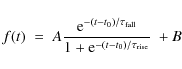
$\begin{displaymath}f(t)\;=\; A \frac{{\rm e}^{-(t-t_0)/\tau_{\rm fall}}}{1+{\rm e}^{-(t-t_0)/\tau_{\rm rise}}} \;+ B \end{displaymath}$

(2)

to obtain estimates of the observed peak luminosities. As SNe Ia are standard candles, a strong correlation is observed between the redshift and the estimated peak flux $f_{\rm max}$ determined from the fit by Eq. (2). This correlation, illustrated in Fig. 3 for the r' band, allowed setting lower (z₁) and upper (z₂) bounds on redshift as well as estimating a mean expected redshift value m_z, along with an uncertainty $\sigma_z$ taken as the r.m.s. dispersion around m_z for a given observed $f_{\rm max}$ . Typical values for $\sigma_z$ lie between 0.06 and 0.11. Two SNe Ia lie outside the limits shown in the figure. One has poor sampling (the first point after peak in any of the four bands occurs after 25 days). The other has both a low stretch ( x₁ = -1.2) and a large intrinsic color (c=0.36, close to our limit of 0.4 for our data sample).

$\begin{figure} \par\includegraphics[width=9cm,clip]{13283fg3.eps} \end{figure}$	Figure 3: Correlation of redshift with the peak flux in r'. Black points are for simulated SNe Ia, red dots for the data sample. The blue curves represent the lower and upper bounds set on redshift, and the green curve the mean estimate of redshift for a given peak flux.
Open with DEXTER

Independent estimates of the redshift bounds z₁ and z₂, mean value m_z and dispersion $\sigma_z$ were computed for the two bands with the best sampling and photometric accuracy, namely r' and i'. As a prior on redshift, we used a Gaussian with mean set to the weighted average of the m_z values from r' and i', and with variance taken to be $[\sigma_z(i')^{-2}+\sigma_z(r')^{-2}]^{-1}$ . The bounds being quite conservative (over $99.5\%$ of the events contained within the limits), the most restrictive ones were retained to limit the range of redshifts probed. The bounds are only useful to reduce the time consumption of the fit and do not lead to further improvement beyond what is already achieved with the prior on redshift.

3.2 Fitting procedure

In the standard use of SALT2, the fit of the light curves is done at known redshift, and it is best to use only the bands which fall in the rest-frame wavelength range between 290 and 700 nm. In the case studied here, as the redshift is a free parameter, all four bands g', r', i' and z' are used at all times. The priors on color, stretch and redshift defined above were used throughout.

The first step of the fit consisted in computing the reduced $\chi^2$ for successive values of the redshift separated by $\delta z = 0.1$ , within the bounds defined as explained above. To reduce the time consumption, this step is done at fixed $c=m_{\rm c}$ and x₁=m_x₁. The value of the redshift $z_{\rm min}\vert _{{\rm c},x_1}$ yielding the minimum reduced $\chi^2$ in this scan was taken as the initial redshift for the second step. In the presence of two minima, both were considered thereafter. Note that with the bounds set on the redshift range, multiple minima only occurred in 3.5% of the events.

A finer tuning of the initial redshift was then obtained by setting the color and stretch parameters free and performing a new redshift scan around $z_{\rm min}\vert _{{\rm c},x_1}$ , with the same step $\delta z$ as above, until a reduced $\chi^2$ minimum was reached. The values of redshift, color and stretch for the fit that yielded the lowest reduced $\chi^2$ were taken as initial values for the full fit. The latter was performed with the standard code of the light curve fitter SALT2, letting all five parameters free and initialized as described above. When two minima were observed in step 1, both were taken into account. The solution with the smallest reduced $\chi^2$ at the end of the full fit was chosen. Note that in 71% of the cases with two $\chi^2$ local minima, both minima ended up with the same set of values for all five parameters (within statistical errors). Only 1% of the events thus truly needed to go through all 3 steps for both $z_{\rm min}\vert _{c,x_1}$ to determine the best redshift.

4 Statistical accuracy of SN Ia photometric redshifts

The performance of the method described above was assessed from the two samples of simulated and observed SN Ia light curves. The photometric redshift was compared with the generated one ( $z_{\rm gen}$ ) for simulated events and with the spectroscopic one ( $z_{\rm spe}$ ) for data.

In both cases, 99% of the events lie within $0.15 \times (1+z)$ of the actual redshift. With the precision defined as in Coupon et al. (2009) by $\sigma_{\Delta z/(1+z)} \equiv 1.48\times{\rm median}[\vert\Delta z\vert/(1+z)]$ (a robust estimate of the r.m.s), and the outlier rate $\eta$ , or rate of catastrophic errors, defined as the proportion of events with $\vert\Delta z\vert/(1+z)>0.15$ , we obtain a precision of 0.022 and $\eta = 1.4\%$ on average over the entire redshift range (see Fig. 4). 10% of the events have $\vert\Delta z\vert/(1+z) > 0.07$ . For 70% of these, the reduced $\chi^2$ is smaller than for the fit initialized at the actual redshift. The photometric redshift therefore appears, wrongly, to be a better solution than the actual redshift. This is a limitation of any method based on $\chi^2$ minimization.

$\begin{figure} \par\includegraphics[width=9cm,clip]{13283fg4.eps} \end{figure}$

Figure 4:

Photometric vs. spectroscopic redshift for the method of this paper. The green lines are for ${z_{\rm pho}}= {z_{\rm spe}}\pm 0.022(1+{z_{\rm spe}})$ representing the average precision over the entire redshift range, and the blue lines for ${z_{\rm pho}}= {z_{\rm spe}}\pm 0.15(1+{z_{\rm spe}})$ to visualize the catastrophic redshifts. Red circles are data SNe Ia for which a spectroscopic redshift is available, black points are the simulated SNe Ia.

Open with DEXTER

The accuracy achieved for two redshift intervals (below and above 0.45) is given in Table 1. The reduced accuracy at high redshift comes from the vanishing SN flux in the g' then r' bands of SNLS, thus enhancing fit degeneracies (see discussion). The redshift dependence of the accuracy is well reproduced by an increase of the spread in $\Delta z$ proportionally to (1+z)², with $\sigma_{\Delta z/(1+z)^2} = 0.014$ independently of redshift.

Table 1: Accuracy $\sigma _{\Delta z/(1+z)}$ of the supernova photometric redshift ${z_{\rm pho}}$ .

Comparison of Cols. 2 and 6 shows that $\eta$ for simulation and data are in agreement, given the uncertainty of 0.7% on $\eta$ for data. Resolutions at high redshift are also in agreement. At low redshift, it is slightly worse for data, probably due to sources of SN Ia heterogeneity not reproduced in the simulation.

As visible in Cols. 5 and 6, the photometric determination of the supernova redshift has very few outliers for spectroscopically confirmed SNe Ia. Most of the catastrophic failures occur for events that have been added by the photometric selection. The increase in $\eta$ between Cols. 5 and 6 is in agreement with the estimated contamination fraction of 1% of the total sample. The precision also tends to be slightly better for spectroscopically confirmed events.

An alternative to supernovae photometric redshifts is to use photometric redshifts of the host galaxies, $z_{\rm gal}$ . Ilbert et al. (2006) have published photometric redshifts for 522286 objects in the four deep fields of SNLS. Only 83% of potential SNe Ia have a matched host with a $z_{\rm gal}$ , while SN Ia photometric redshifts can be computed for all objects. The two photometric redshift determinations are compared in the last two columns of Table 1. Supernova photometric redshifts have a much better precision. However, when combined with a photometric selection of SNe Ia, it may lead to samples more contaminated by core-collapse supernovae for instance than when using galactic photometric redshifts which are independent of the light curves. Future projects might want to combine the two techniques to obtain a selection of SNe Ia with reduced contamination from non-Ia supernovae (using fits with redshift fixed at $z_{\rm gal}$ to obtain the selected sample of SNe Ia) while having the redshift accuracy of supernovae photometric redshifts (refitting the redshift of the selected events to derive ${z_{\rm pho}}$ ).

5 Discussion

As illustrated in Cols. 1 and 2 (for the simulation) or 4 and 6 (for the data) of Table 1, the prior set on redshift reduces the rate of catastrophic errors by $\sim$ 1.5%. Their impact on precision, however, is small, because the precision attained is significantly better than the width $\sigma_z$ of the prior.

We have also checked the impact of assuming that SNe Ia are ``normal'' by removing all the priors on color, stretch and redshift but maintaining the same fitting procedure, i.e. two consecutive $\chi^2$ scans to initialize the values of the parameters for the full fit. The precision obtained on average over the entire redshift range is then of 0.029 and the rate of outliers is significantly increased to $\eta = 9.6\%$ . Most of these accidental fits end with extreme colors (c>2) assigned to the events. The assumption that SNe Ia are normal therefore improves slightly the accuracy (by $\sim$ 25%) but is crucial to reach a small rate of accidental redshifts (reduction by factor $\sim$ 10).

As inaccurate redshifts were correlated with inaccurate colors, we tried to replace the statistical prior on color by an estimate of the color of each event based on its four-band photometry. This led to little improvement due to the large dispersion around this estimate (often larger than $\sigma_{\rm c} = 0.15$ observed statistically on the sample of data SNe Ia). We thus remained with the prior $m_{\rm c} = 0.04$ and $\sigma_{\rm c} = 0.15$ .

Despite the initialization procedure through two consecutive $\chi^2$ scans, some redshifts are still favored over others. To understand the origin of this problem, two tests were performed.

The first one consisted in applying the procedure to perfect simulated light curves with a sampling of one point per night and no flux dispersion. The redshift was determined with an accuracy $\sigma_{\Delta z /(1+z)}<0.001$ over the full redshift range with no redshift favored (Fig. 5, top plot).

$\begin{figure} \par\includegraphics[width=9cm,clip]{13283fg5.eps} \end{figure}$	Figure 5: Photometric vs. generated redshift for simulated supernovae with perfect photometry. Time sampling is one point per day (top plot) or as in SNLS data (bottom plot, with a different scale). Lines indicate redshifts which tend to be favored by the fit. Results from sampling with one point per day superimposed on bottom plot as open green circles.
Open with DEXTER

$\begin{figure} \par\includegraphics[width=9cm,clip]{13283fg6.eps} \end{figure}$	Figure 6: Generated colors as a function of generated redshift. Shown in each plot are the events with a magnitude brighter than 25 in the two concerned filters. Lines indicate redshifts which tend to be favored by the fit.
Open with DEXTER

In the second test, the light curves still had perfect photometry but the sampling was degraded to reproduce that of real data. While the accuracy remained excellent, some accumulations (bottom plot of Fig. 5) appeared at the same values of ${z_{\rm pho}}$ as with the full simulation of Fig. 4. The $z\sim 0.47$ and $z\sim 0.80$ accumulations correspond to turn-overs in the r-i vs. redshift diagram (cf. Fig. 6). The smaller one at $z\sim 0.60$ corresponds to a short plateau. Since SALT2 fits light curve colors, and as the r' and i' bands are the ones which contribute the most (best sampling and S/N), double redshift values for a given r-i color can indeed lead to the observed degeneracies. The first two can partially be broken with data in the g' band since the g-r vs. redshift diagram is monotonic (this also explains why the turn-over at $z\sim 0.3$ does not lead to redshift accumulations). This is not the case for $z\sim 0.8$ where there is no longer any significant flux in the g' band.

Note that when reaching perfect photometry, the data $\chi^2$ vanishes for the generated values of the fitted parameters and the priors then play a major role. In the case of redshift degeneracies, the fit converges to the redshift (out of the two possible ones) that minimizes the contribution of the color and stretch priors. Thus, near ${z_{\rm pho}}\sim 0.8$ , events with large/small intrinsic colors tend to be fitted with over-/under-estimated redshifts. With more data points in a third band (i.e. other than r' and i'), the contribution of the priors to the total $\chi^2$ becomes negligible and the fit is truly constrained by the data only. As shown in the top plot of Fig. 5, a sampling of 1 point every day in all four bands fully breaks the degeneracies.

$\begin{figure} \par\includegraphics[width=9cm,clip]{13283fg7.eps} \end{figure}$	Figure 7: Accuracy of the redshift determination in the full simulation (solid curve) and in the simulation with perfect photometry but time sampling as in the data (dashed curve). Mean and rms are given for the full simulation.
Open with DEXTER

As illustrated in Fig. 7, the main impact of the photometric uncertainties is to reduce the accuracy with which the redshift is determined by increasing the width of the ${z_{\rm pho}}\sim {z_{\rm spe}}$ band. Note that the distributions are non-Gaussian, which justifies the use of a median-based estimate of the rms (Sect. 4). We have verified that the region thus defined does include at least $68\%$ of the simulated events whatever the redshift range up to $z\sim 1.1$ .

SALT2 requires no assumption on cosmology. A dependence on cosmology could only come from the bounds and prior on redshift. This was tested by simulating SNe Ia in a flat $\Omega_{\rm M} =1$ Universe where the SNe Ia are more luminous by $\sim$ 0.5 mag at z=0.6. The bounds are sufficiently loose to be valid even in that extreme case. The prior on redshift is systematically underestimated by $\sim$ 0.1, but at the end of the fitting procedure we obtain no bias and the same precision and outlier rate as in Table 1 Col. 2. The only difference is that outliers are more often under- than over-estimates of the redshift.

6 Uncertainties and biases

Although the photometric redshift shows negligible bias on average ( $\langle {z_{\rm pho}}- {z_{\rm spe}}\rangle =0.003$ ), there is a clear correlation between color and redshift biases: overestimated redshifts are systematically correlated with underestimated colors.

Supernovae with z<0.6 have non-zero flux in at least 3 bands and usually end up with good estimates of both redshift and color. As the redshift increases however, the loss of information (due to unmeasurably small fluxes in the bluest bands) gives increasingly more weight to the color prior compared to the data. The fitted color thus tends to converge to that of the prior ( $m_{\rm c}$ ), leading to a color-dependent bias (cf. Fig. 8). This is particularly clear near redshift degeneracies (cf. Fig. 4), where events with positive (resp. negative) intrinsic colors populate the ${z_{\rm pho}}> z_{\rm gen}$ (resp. ${z_{\rm pho}}< z_{\rm gen}$ ) accumulations.

$\begin{figure} \par\includegraphics[width=9cm,clip]{13283fg8.eps} \end{figure}$	Figure 8: Redshift bias as a function of the supernova intrinsic color for three redshift bins: red squares for z<0.45, filled black circles for 0.45<z<0.65 and open blue circles for z>0.65. The vertical lines delimit the 1 $\sigma$ color range.
Open with DEXTER

$\begin{figure} \par\includegraphics[width=9cm,clip]{13283fg9.eps} \end{figure}$

Figure 9:

Top: bias on redshift as a function of the fitted redshift with the additional SALT2 fit for three bins of intrinsic (generated) color $c_{\rm gen}$ : black squares for $\vert c_{\rm gen}-m_{\rm c}\vert<0.1$ , filled red circles for $c_{\rm gen}-m_{\rm c}>0.1$ and open blue circles for $c_{\rm gen}-m_{\rm c}<-0.1$ . The curves illustrate the 0.014(1+z)² statistical uncertainty. Bottom: bias on color as a function of the fitted redshift. Same color code as above.

Open with DEXTER

To reduce this bias and improve the color and redshift determination for ``colored'' SNe ( $\vert c_{\rm gen}-m_{\rm c}\vert > 0.1$ where $c_{\rm gen}$ is the generated color) in SNLS, we performed an additional SALT2 fit as follows: the mean and $\sigma$ of the Gaussian prior on x₁ are set to the best fit value of x₁ and its uncertainty from the procedure of Sect. 3, a Gaussian prior on redshift is used with mean set to the value found previously and $\sigma$ taken as $0.014\times (1+{z_{\rm pho}})^2$ . With these stronger constraints, we eliminate the prior on color.

Above a redshift of 0.65, the additional fit reduces the bias $z_{\rm pho} - z_{\rm gen}$ by $\sim$ 0.02 for blue SNe ( $c_{\rm gen}-m_{\rm c}<-0.1$ ) while yielding a smaller but systematic improvement on red ( $c_{\rm gen}-m_{\rm c}>0.1$ ) SNe. The color determination is also systematically improved: above a redshift of 0.65, the color bias is reduced by 0.04 for blue SNe and by 0.01 for red ones. Fits to events with $c_{\rm gen}\sim m_{\rm c}$ (black squares in Fig. 9), or to low redshift events where the data have more weight than the priors, are unchanged: these events were already well fitted.

Figure 9 illustrates the remaining bias on fitted redshift or fitted color as a function of redshift, for several ranges of intrinsic color. At high redshift, the reddest (and thus also the faintest) SNe exhibit the largest bias, emphasizing the lack of another filter (beyond the z band) with measurable flux to determine the SN parameters. On average for events passing the preselection filter, however, the bias remains small, with ${z_{\rm pho}}-{z_{\rm gen}}< 0.027$ whatever the redshift up to a $z\sim 1.1$ , and $\langle {z_{\rm pho}}-{z_{\rm gen}}\rangle = 0.008$ on average over the full redshift range between 0 and 1.1. The statistical uncertainty derived in Sect. 4 is indicated in Fig. 9. It encompasses about 68% of the events at all redshifts.

7 Conclusions

The study presented in this paper shows that SN Ia photometric redshifts can be obtained with an accuracy exceeding that of current host galaxy photometric redshifts. The method was applied to simulated light curves as well as to a sample of SNe Ia from the first three years of SNLS data for which the redshift was known from spectroscopy. The accuracy reaches $\sigma_{\Delta z/(1+z)} = 0.022$ on average over the entire redshift range, with $\sigma_{\Delta z/(1+z)} = 0.016$ for z<0.45 and $\sigma_{\Delta z/(1+z)} = 0.025$ for 0.45<z<1.1. Degeneracies in the fit above $z \sim 0.45$ , due to vanishing flux in the bluest band of SNLS, are responsible for the lower accuracy at high redshifts. The spread in $\Delta z /(1+z)^2$ is seen to be independent of redshift, with $\sigma_{\Delta z/(1+z)^2} = 0.014$ .

Red (resp. blue) SNe tend to have an overestimated (resp. underestimated) redshift. The net bias however on the fitted redshift, after integration over the SN population, remains smaller than 0.027 whatever the redshift up to $z\sim 1.1$ , with a net bias $\langle {z_{\rm pho}}-{z_{\rm gen}}\rangle$ of 0.008 on average.

For only 1.4% of the events do we obtain a catastrophic error ( $\vert\Delta z\vert/(1+z)>0.15$ ) on the estimate of the redshift, and for 10% an error larger than 0.07. The rate of catastrophic failures is reduced to 0.4% for spectroscopically confirmed SNe Ia.

The method is illustrated with SNLS data but can be adapted to other supernova samples.

Acknowledgements

SNLS relies on observations with MegaCam, a joint project of CFHT and CEA/DAPNIA, at the Canada-France-Hawaii Telescope (CFHT) which is operated by the National Research Council (NRC) of Canada, the Institut National des Science de l'Univers of the Centre National de la Recherche Scientifique (CNRS) of France, and the University of Hawaii. This work is based in part on data products produced at the Canadian Astronomy Data Centre as part of the Canada-France-Hawaii Telescope Legacy Survey, a collaborative project of the National Research Council of Canada and the French Centre national de la recherche scientifique. SNLS also relies on observations obtained at the European Southern Observatory using the Very Large Telescope on the Cerro Paranal (ESO Large Programme 171.A-0486), on observations (programs GN-2006B-Q-10, GN-2006A-Q-7, GN-2005B-Q-7, GS-2005B-Q-6, GN-2005A-Q-11, GS-2005A-Q-11, GN-2004B-Q-16, GS-2004B-Q-31, GN-2004A-Q-19, GS-2004A-Q-11, GN-2003B-Q-9, and GS-2003B-Q-8) obtained at the Gemini Observatory, which is operated by the Association of Universities for Research in Astronomy, Inc., under a cooperative agreement with the NSF on behalf of the Gemini partnership: the National Science Foundation (United States), the Particle Physics and Astronomy Research Council (United Kingdom), the National Research Council (Canada), CONICYT (Chile), the Australian Research Council (Australia), CNPq (Brazil) and CONICET (Argentina), and on observations obtained at the W. M. Keck Observatory, which is operated as a scientific partnership among the California Institute of Technology, the University of California and the National Aeronautics and Space Administration. The Observatory was made possible by the generous financial support of the W. M. Keck Foundation. MS acknowledges support from the Royal Society.

References

Astier, P., Guy, J., Regnault, N., et al. 2006, A&A, 447, 31 [NASA ADS] [CrossRef] [EDP Sciences] [Google Scholar]
Balland, C., Baumont, S., Basa, S., et al. 2009, A&A, 507, 85 [NASA ADS] [CrossRef] [EDP Sciences] [Google Scholar]
Bronder, J., Hook, I. M., Astier, P., et al. 2008, A&A, 477, 717 [NASA ADS] [CrossRef] [EDP Sciences] [Google Scholar]
Coupon, J., Ilbert, O., Kilbinger, M., et al. 2009, A&A, 500, 981 [NASA ADS] [CrossRef] [EDP Sciences] [Google Scholar]
Ellis, R. S., Sullivan, M., Nugent, P. E., et al. 2008, ApJ, 674, 51 [NASA ADS] [CrossRef] [Google Scholar]
Guy, J., Astier, P., Baumont, S., et al. 2007, A&A, 466, 11G [NASA ADS] [CrossRef] [EDP Sciences] [Google Scholar]
Howell, A., Conley, M., Della Valle, P. E., et al. 2009 [arXiv:0903.1086] [Google Scholar]
Howell, A., Sullivan, M., Perrett, K., et al. 2005, AJ, 634, 1190 [NASA ADS] [CrossRef] [Google Scholar]
Ilbert, O., Arnouts, S., McCracken, H. J., et al. 2006, A&A, 457, 841I [NASA ADS] [CrossRef] [EDP Sciences] [Google Scholar]
Sullivan, M., Howell, D. A., Perrett, K., et al. 2006, AJ, 131, 960 [NASA ADS] [CrossRef] [Google Scholar]
Wang, Y. 2007, AJ, 654, L123 [NASA ADS] [CrossRef] [Google Scholar]

Footnotes

... package: http://wwwasdoc.web.cern.ch/wwwasdoc/minuit/minmain.html
... range: SALT2 was trained with 40% of the data used here. Restricting to the complementary set yields results in agreement with the quoted performances within statistical uncertainties.
... redshift: Note that the $\chi^2$ comparison is done on the sole contribution of the data points (i.e. not including the contribution of the priors), as there is no redshift prior for the fit initialized at the actual redshift.
... host: The match to a host galaxy was considered successful out to a supernova-host distance of $5~r_{\rm gal}$ with $r_{\rm gal}$ defined as the half-width of the galaxy in the direction of the event. 9% of the SNe lie in regions masked in the galaxy catalog because of neighboring bright stars, and 9% of the remaining SNe are associated to a galaxy lacking a secure $z_{\rm gal}$ for diverse photometric reasons.

All Tables

Table 1: Accuracy $\sigma _{\Delta z/(1+z)}$ of the supernova photometric redshift ${z_{\rm pho}}$ .

All Figures

$\begin{figure} \par\includegraphics[width=9cm,clip]{13283fg1.eps} \vspace*{2mm} \end{figure}$	Figure 1: Color distribution of SNe Ia with redshift z<0.7 from the first three years of SNLS data. The curve is a fit to the data with a double Gaussian as explained in the text.
Open with DEXTER
In the text

$\begin{figure} \par\includegraphics[width=9cm,clip]{13283fg2.eps} \end{figure}$	Figure 2: Photometric vs. spectroscopic redshift for the data sample in the absence of initialization or prior on redshift.
Open with DEXTER
In the text

$\begin{figure} \par\includegraphics[width=9cm,clip]{13283fg3.eps} \end{figure}$	Figure 3: Correlation of redshift with the peak flux in r'. Black points are for simulated SNe Ia, red dots for the data sample. The blue curves represent the lower and upper bounds set on redshift, and the green curve the mean estimate of redshift for a given peak flux.
Open with DEXTER
In the text

$\begin{figure} \par\includegraphics[width=9cm,clip]{13283fg4.eps} \end{figure}$	Figure 4: Photometric vs. spectroscopic redshift for the method of this paper. The green lines are for ${z_{\rm pho}}= {z_{\rm spe}}\pm 0.022(1+{z_{\rm spe}})$ representing the average precision over the entire redshift range, and the blue lines for ${z_{\rm pho}}= {z_{\rm spe}}\pm 0.15(1+{z_{\rm spe}})$ to visualize the catastrophic redshifts. Red circles are data SNe Ia for which a spectroscopic redshift is available, black points are the simulated SNe Ia.
Open with DEXTER
In the text

$\begin{figure} \par\includegraphics[width=9cm,clip]{13283fg5.eps} \end{figure}$	Figure 5: Photometric vs. generated redshift for simulated supernovae with perfect photometry. Time sampling is one point per day (top plot) or as in SNLS data (bottom plot, with a different scale). Lines indicate redshifts which tend to be favored by the fit. Results from sampling with one point per day superimposed on bottom plot as open green circles.
Open with DEXTER
In the text

$\begin{figure} \par\includegraphics[width=9cm,clip]{13283fg6.eps} \end{figure}$	Figure 6: Generated colors as a function of generated redshift. Shown in each plot are the events with a magnitude brighter than 25 in the two concerned filters. Lines indicate redshifts which tend to be favored by the fit.
Open with DEXTER
In the text

$\begin{figure} \par\includegraphics[width=9cm,clip]{13283fg7.eps} \end{figure}$	Figure 7: Accuracy of the redshift determination in the full simulation (solid curve) and in the simulation with perfect photometry but time sampling as in the data (dashed curve). Mean and rms are given for the full simulation.
Open with DEXTER
In the text

$\begin{figure} \par\includegraphics[width=9cm,clip]{13283fg8.eps} \end{figure}$	Figure 8: Redshift bias as a function of the supernova intrinsic color for three redshift bins: red squares for z<0.45, filled black circles for 0.45<z<0.65 and open blue circles for z>0.65. The vertical lines delimit the 1 $\sigma$ color range.
Open with DEXTER
In the text

$\begin{figure} \par\includegraphics[width=9cm,clip]{13283fg9.eps} \end{figure}$	Figure 9: Top: bias on redshift as a function of the fitted redshift with the additional SALT2 fit for three bins of intrinsic (generated) color $c_{\rm gen}$ : black squares for $\vert c_{\rm gen}-m_{\rm c}\vert<0.1$ , filled red circles for $c_{\rm gen}-m_{\rm c}>0.1$ and open blue circles for $c_{\rm gen}-m_{\rm c}<-0.1$ . The curves illustrate the 0.014(1+z)² statistical uncertainty. Bottom: bias on color as a function of the fitted redshift. Same color code as above.
Open with DEXTER
In the text

Current usage metrics show cumulative count of Article Views (full-text article views including HTML views, PDF and ePub downloads, according to the available data) and Abstracts Views on Vision4Press platform.

Data correspond to usage on the plateform after 2015. The current usage metrics is available 48-96 hours after online publication and is updated daily on week days.

Initial download of the metrics may take a while.