| Issue |
A&A
Volume 514, May 2010
|
|
|---|---|---|
| Article Number | A88 | |
| Number of page(s) | 13 | |
| Section | Cosmology (including clusters of galaxies) | |
| DOI | https://doi.org/10.1051/0004-6361/200912654 | |
| Published online | 26 May 2010 | |
Abell 611
I. Weak lensing analysis with LBC
A. Romano1,2 - L. Fu3,12 - F. Giordano4,2 - R. Maoli1 - P. Martini5 - M. Radovich3,14 - R. Scaramella2 - V. Antonuccio-Delogu6,13 - A. Donnarumma7,8,9 - S. Ettori8,9 - K. Kuijken10,3 - M. Meneghetti8,9 - L. Moscardini7,9 - S. Paulin-Henriksson11,6 - E. Giallongo2 - R. Ragazzoni14 - A. Baruffolo14 - A. DiPaola2 - E. Diolaiti8 - J. Farinato14 - A. Fontana2 - S. Gallozzi2 - A. Grazian2 - J. Hill 16 - F. Pedichini2 - R. Speziali2 - R. Smareglia15 - V. Testa2
1 - Dipartimento di Fisica, Universitá La Sapienza, piazzale A. Moro 2,
00185 Roma, Italy
2 - INAF - Osservatorio Astronomico di Roma, via Frascati 33, 00044
Monte Porzio Catone (Roma), Italy
3 - INAF - Osservatorio Astronomico di Napoli, via Moiariello
16, 80131 Napoli, Italy
4 - Dipartimento di Fisica, Universitá Tor Vergata, via della Ricerca
Scientifica 1, 00133 Roma, Italy
5 - Department of Astronomy and Center for Cosmology and Astroparticle
Physics, The Ohio State University, Columbus, OH 43210, USA
6 - INAF - Osservatorio Astrofisico di Catania, via Santa Sofia 78,
95123 Catania, Italy
7 - Dipartimento di Astronomia, Universitá di Bologna, via
Ranzani 1, 40127 Bologna, Italy
8 - INAF - Osservatorio Astronomico di Bologna, via
Ranzani 1, 40127 Bologna, Italy
9 - INFN, Sezione di Bologna, viale Berti Pichat 6/2, 40127 Bologna,
Italy
10 - Leiden Observatory, Leiden University, PO Box 9513, 2300
RA Leiden, The Netherlands
11 - Service d'Astrophysique, CEA Saclay, Batiment 709, 91191
Gif-sur-Yvette Cedex, France
12 - Key Lab for Astrophysics, Shanghai Normal University, 100 Guilin
Road, 200234 Shanghai, PR China
13 - Astrophysics, Department of Physics, University of Oxford, Oxford,
UK
14 - INAF - Osservatorio Astronomico di Padova, vicolo
dell'Osservatorio 5, 35122 Padova, Italy
15 - INAF - Osservatorio Astronomico di Trieste, via G. B. Tiepolo 11,
34131 Trieste, Italy
16 - Large Binocular Telescope Observatory, University of Arizona, 933
N Cherry Avenue, 85721-0065 Tucson, Arizona, USA
Received 8 June 2009 / Accepted 3 February 2010
Abstract
Aims. The Large Binocular Cameras (LBC) are two twin
wide field cameras (FOV ![]() )
mounted at the prime foci of the 8.4 m Large Binocular
Telescope (LBT). We performed a weak lensing analysis of the z=0.288
cluster Abell 611 on g-band data obtained
by the blue-optimized LBC in order to estimate the cluster mass.
)
mounted at the prime foci of the 8.4 m Large Binocular
Telescope (LBT). We performed a weak lensing analysis of the z=0.288
cluster Abell 611 on g-band data obtained
by the blue-optimized LBC in order to estimate the cluster mass.
Methods. Owing to the complexity of the PSF of LBC,
we decided to use two different approaches, KSB and shapelets, to
measure the shape of background galaxies and to derive the shear signal
produced by the cluster. Then we estimated the cluster mass with both
aperture densitometry and parametric model fits.
Results. The combination of the large aperture of
the telescope and the wide field of view allowed us to map a region
well beyond the expected virial radius of the cluster and to get a high
surface density for background galaxies (23 galaxies/arcmin2).
This made it possible to estimate an accurate mass for
Abell 611. We find that the mass within 1.5 Mpc is ![]() from the aperture mass technique and
from the aperture mass technique and ![]() using the model fitting by an NFW mass density profile for both
shapelet and KSB methods. This analysis demonstrates that LBC is a
powerful instrument for weak gravitational lensing studies.
using the model fitting by an NFW mass density profile for both
shapelet and KSB methods. This analysis demonstrates that LBC is a
powerful instrument for weak gravitational lensing studies.
Key words: galaxies: clusters: individual: Abell 611 - gravitational lensing: weak
1 Introduction
According to the hierarchical model of structure formation, clusters of galaxies are the most massive objects in the universe, and the cluster mass function is a powerful probe of cosmological parameters (e.g. Evrard 1989; Eke et al. 1998; Vikhlinin et al. 2009; Allen et al. 2004; Henry 2000). In addition, the ratio between the cluster gas mass, as estimated with X-ray observations, and the total mass in a galaxy cluster provides stringent constraints on the total matter density. Specifically, the apparent evolution of the gas fraction with redshift can be used to estimate the contribution of the dark energy component to the cosmic density (e.g. Allen et al. 2008; Ettori et al. 2009). Using clusters as a cosmological probe therefore requires reliable mass estimates.
Several techniques are commonly used to estimate masses for galaxy clusters: the X-ray luminosity or temperature of the hot intracluster gas, the Sunyaev-Zel'dovich effect, the number of bright galaxies in a cluster, and the velocity dispersion of the cluster galaxies. The disadvantage of all these methods is that they are indirect and require significant assumptions about the dynamical state of the cluster. Gravitational lensing, in contrast, is only sensitive to the amount of mass along the line of sight and allows reconstruction of the projected cluster mass regardless of its composition or dynamical behavior (e.g. Kaiser & Squires 1993). The only direct method of estimating cluster masses is therefore via measuring the distortion (shear) of the shapes of background galaxies that are weakly lensed by the gravitational potential of the cluster.
This distortion is very small and lensed galaxies are usually
at high redshift. Observational studies to measure weak gravitational
lensing by clusters require deep images in order to detect these faint
sources and to obtain a high number density of background galaxies.
Moreover, this kind of analysis requires very high-quality images to
measure the shape of the lensed sources with high precision: good
seeing (<
![]() )
conditions and a high signal-to-noise ratio (SNR typically >10)
are needed. Wide-field images are also required to obtain a statistical
measure of the tangential shear as a function of distance from the
cluster center so that the projected mass measured by weak lensing
essentially includes all of the mass of the cluster (Clowe &
Schneider 2001,2002).
)
conditions and a high signal-to-noise ratio (SNR typically >10)
are needed. Wide-field images are also required to obtain a statistical
measure of the tangential shear as a function of distance from the
cluster center so that the projected mass measured by weak lensing
essentially includes all of the mass of the cluster (Clowe &
Schneider 2001,2002).
In the past decade substantial progress has been made with weak lensing studies thanks to the advent of wide-field data with linear detectors, the development of sophisticated algorithms for shape measurements (e.g. Kaiser et al. 1995; Bernstein & Jarvis 2002; Refregier 2003; Kuijken 2006), and the availability of multi-band photometry, which provides information about the redshift distribution of the lensed sources (Ilbert et al. 2006).
Here we describe the results of a weak lensing analysis of the
Abell 611 cluster. This analysis is based on images
obtained with the Large Binocular Camera (LBC), which are a
pair of prime focus cameras mounted on the two 8.4 m diameter
mirrors of the Large Binocular Telescope (LBT). Each LBC has a
![]() field
of view (FOV) and, combined with the collecting area of LBT, is a very
powerful instrument for weak lensing studies.
field
of view (FOV) and, combined with the collecting area of LBT, is a very
powerful instrument for weak lensing studies.
Abell 611 is a rich cluster at redshift z=0.288 (Struble & Rood 1999) that appears relaxed in X-ray data, has a regular morphology, and the brightest cluster galaxy (BCG) is coincident with the center of X-ray emission (Donnarumma et al. 2010). A giant arc caused by strong lensing is also clearly visible close to the BCG (Fig. 1).
![\begin{figure}
\par\includegraphics[width=8cm,clip]{12654fg1.ps}
\end{figure}](/articles/aa/full_html/2010/06/aa12654-09/img21.png)
|
Figure 1:
A three-color image (
|
| Open with DEXTER | |
In this work we describe a weak lensing analysis to estimate the mass of Abell 611 from a deep g-band LBC image whose field of view extends well beyond the expected virial radius of the cluster. We compare the mass estimated from gravitational lensing with previous lensing results and with other mass estimates available in the literature that were derived by secondary techniques. In particular, we compare our weak lensing results with new mass measurements obtained by X-ray analysis of Chandra data provided to us by Donnarumma et al. (2010).
Mass measurements by weak lensing do not need any assumption about the geometry of the cluster; however, assumptions are required to compare projected lensing masses with other mass estimates. Thus projection effects have to be taken into account during this kind of analysis; in particular, the true triaxiality of the halo (De Filippis et al. 2005; Gavazzi 2005) and the presence of unrelated structures along the line of sight (Metzler et al. 2001; Hoekstra 2007) can be sources of noise or bias on the projected mass measurements.
The paper is organized as follows. In the first sections we describe the data (Sect. 2) used for a weak lensing analysis of Abell 611, the catalog extraction of the background sources (Sect. 3), and the selection of candidate cluster galaxies (Sect. 4). The two different pipelines used to extract the shear signal from the images are described in Sect. 5, and their results are compared in Sect. 5.3. Finally, both shear maps are used to estimate the mass of the cluster with different techniques (Sect. 6). The results are summarized and discussed in Sect. 7.
Throughout this paper we adopt H0
= 70 km s-1 Mpc-1,
![]() ,
and
,
and ![]() .
At the distance of Abell 611, 1 arcmin corresponds to
a projected physical distance of nearly 0.26 Mpc.
.
At the distance of Abell 611, 1 arcmin corresponds to
a projected physical distance of nearly 0.26 Mpc.
![\begin{figure}
\par\includegraphics[width=8cm,clip]{12654fg2.ps}
\end{figure}](/articles/aa/full_html/2010/06/aa12654-09/img24.png)
|
Figure 2: g-band image of the full field of LBC, centered on Abell 611. The box marks the region of 5000 pixels we used for the analysis. |
| Open with DEXTER | |
2 Observations and data reduction
Abell 611 was observed in March 2007, during the science
demonstration time (SDT) for the blue-optimized large binocular
camera (LBC), which is one of the two LBCs built for the prime
foci of the LBT. The LBC focal plane consists of four CCDs (
![]() pixels, pixel scale
13.5
pixels, pixel scale
13.5 ![]() m,
gain
m,
gain ![]() 2 e-/ADU,
readout-noise
2 e-/ADU,
readout-noise ![]() 11 e-).
The CCDs are arranged so that three of the chips are butted along their
long edges and the fourth chip is rotated counterclockwise by
90 degrees and centered on the top of the other CCDs (see
Fig. 2).
The field of view is equivalent to
11 e-).
The CCDs are arranged so that three of the chips are butted along their
long edges and the fourth chip is rotated counterclockwise by
90 degrees and centered on the top of the other CCDs (see
Fig. 2).
The field of view is equivalent to ![]() and provides images with a sampling of 0.225''/pixel. Because each LBC
is mounted on a swing arm over the primary mirror, the support
structure lacks the symmetry of most prime focus instruments. Moreover
LBC PSFs are dominated by optical aberrations from misalignments, which
can prevent PSFs from having bilateral symmetry.
This is a potential complication for the weak lensing analysis, a point
we discuss below. More details about the characteristics of LBC are
given in Giallongo et al.
(2008).
and provides images with a sampling of 0.225''/pixel. Because each LBC
is mounted on a swing arm over the primary mirror, the support
structure lacks the symmetry of most prime focus instruments. Moreover
LBC PSFs are dominated by optical aberrations from misalignments, which
can prevent PSFs from having bilateral symmetry.
This is a potential complication for the weak lensing analysis, a point
we discuss below. More details about the characteristics of LBC are
given in Giallongo et al.
(2008).
The observations, collected in optimal seeing conditions (
![]() ), consisted of several sets
of exposures of 5 min each in a wide u-band
and in SDSS g- and r-band
filters. The total exposure time was 1 h in g,
15 min in r, and 20 min in u.
For the present work we used the deep, g-band data
for the weak-lensing analysis and the u- and r-band
data to select cluster galaxies. Each image was dithered by
5 arcsec to remove bad pixels, rows, columns, and satellite
tracks. This offset is not large enough to fill the gaps between the
CCDs, but the analysis plan was to treat CCDs separately owing to
expected PSF discontinuities at the chip boundaries. The offsets were
therefore kept small to maximize depth and uniformity.
), consisted of several sets
of exposures of 5 min each in a wide u-band
and in SDSS g- and r-band
filters. The total exposure time was 1 h in g,
15 min in r, and 20 min in u.
For the present work we used the deep, g-band data
for the weak-lensing analysis and the u- and r-band
data to select cluster galaxies. Each image was dithered by
5 arcsec to remove bad pixels, rows, columns, and satellite
tracks. This offset is not large enough to fill the gaps between the
CCDs, but the analysis plan was to treat CCDs separately owing to
expected PSF discontinuities at the chip boundaries. The offsets were
therefore kept small to maximize depth and uniformity.
The images were reduced by the LBT pipeline![]() implemented at INAF-OAR.
The flat-field correction was done using both a twilight flat-field and
a superflat obtained during the night. Moreover, a geometric distortion
correction was performed to normalize the pixel size, which showed
differences across the CCDs caused by field distortions in the optics.
The astrometric solution was computed using the ASTROMC
package (Radovich et al. 2008).
This solution was then used to resample and coadd the images using the
SWARP
implemented at INAF-OAR.
The flat-field correction was done using both a twilight flat-field and
a superflat obtained during the night. Moreover, a geometric distortion
correction was performed to normalize the pixel size, which showed
differences across the CCDs caused by field distortions in the optics.
The astrometric solution was computed using the ASTROMC
package (Radovich et al. 2008).
This solution was then used to resample and coadd the images using the
SWARP![]() software.
software.
Standard fields for photometric calibration were not observed
during the SDT, so we used the values of zero points for each band
(Table 1)
given by Giallongo et al.
(2008). Table 1 also shows
the limiting magnitudes estimated from the faintest point-like objects
detected at the 5![]() and 20
and 20![]() level.
level.
Table 1: Exposure times, limiting magnitudes for point-like sources and zero points (AB) for the observations in each band.
3 Catalog extraction
The detection of sources was performed using the SEXTRACTOR
package (Bertin & Arnouts 1996).
Regions of
the image presenting potential problems, such as spikes and halos
around bright
stars, were masked by visual inspection, and sources inside such
regions were discarded from the final catalog.
In addition, we removed sources located at the borders of each CCD,
where the
SNR was lower due to the small dither offset. Finally, a very bright
star
dominates one of the CCDs. We therefore decided to limit our analysis
to a box (displayed in Fig. 2) with a size of
5000 pixels (corresponding to ![]() 18.7') centered on
Abell 611. Starting from this box of 350 arcmin2,
the effective area used for the analysis was
18.7') centered on
Abell 611. Starting from this box of 350 arcmin2,
the effective area used for the analysis was ![]() 290 arcmin2
after removing all the masked regions (30% due to bright stars, 70% due
to regions between adjacent CCDs with no data or low SNR).
290 arcmin2
after removing all the masked regions (30% due to bright stars, 70% due
to regions between adjacent CCDs with no data or low SNR).
![\begin{figure}
\par\includegraphics[height=8cm,angle=-90]{12654fg3.ps}
\end{figure}](/articles/aa/full_html/2010/06/aa12654-09/img30.png)
|
Figure 3:
Magnitude (g) vs. half-light radius ( |
| Open with DEXTER | |
The separation between stars and galaxies was performed in the mag
![]() plane,
where magnitudes (mag) and half-light radii (
plane,
where magnitudes (mag) and half-light radii (![]() )
were obtained from the
MAG_AUTO and FLUX_RADIUS parameters computed by SEXTRACTOR.
Unsaturated stars were selected on the vertical branch (see
Fig. 3)
in the range 20 < g
< 23 mag and
)
were obtained from the
MAG_AUTO and FLUX_RADIUS parameters computed by SEXTRACTOR.
Unsaturated stars were selected on the vertical branch (see
Fig. 3)
in the range 20 < g
< 23 mag and
![]() pixels. In this way
we obtained 302 stars for the PSF
correction, with an SNR >200 for the
faintest ones.
pixels. In this way
we obtained 302 stars for the PSF
correction, with an SNR >200 for the
faintest ones.
For the lensing analysis, only background galaxies located at redshifts higher than z=0.288, the redshift of the cluster, should be used. Unfortunately, in our case the number of available bands does not allow us to estimate accurate photometric redshifts of these faint galaxies. The selection of the background galaxies was therefore done by choosing an adequate cut in apparent magnitude.
The choice of the upper magnitude limit was based on the
galaxy redshift
distribution obtained by Ilbert
et al. (2006) from the Canada-France-Hawaii
Telescope Legacy Survey (CFHTLS), which also used the SDSS photometric
system. Taking the accuracy of the photometric redshifts (3%)
of Ilbert et al. (2006)
into account, the approximations
due to the different bands they used compared to ours, and the
assumption that we have the same galaxy distribution
in our field, we chose 0.4 as the redshift reference value to
perform the magnitude cut.
Galaxies with ![]() were assumed to belong to the cluster or be foreground galaxies. This
reference value was chosen to be greater than cluster redshift, in
order to reduce the contamination of foreground galaxies as much as
possible, taking the approximations discussed above into account.
were assumed to belong to the cluster or be foreground galaxies. This
reference value was chosen to be greater than cluster redshift, in
order to reduce the contamination of foreground galaxies as much as
possible, taking the approximations discussed above into account.
Figure 4
shows the fraction of the total CFHTLS sources at
![]() (upper panel) and the fraction of background
galaxies at z > 0.4 (bottom panel)
as a function of the apparent magnitude cut.
From this figure we conclude that a magnitude cut at g>23
is a good compromise to minimize the contamination from likely
foreground and cluster galaxies (
(upper panel) and the fraction of background
galaxies at z > 0.4 (bottom panel)
as a function of the apparent magnitude cut.
From this figure we conclude that a magnitude cut at g>23
is a good compromise to minimize the contamination from likely
foreground and cluster galaxies (![]() 10%) and to maximize the
number density of background galaxies (
10%) and to maximize the
number density of background galaxies (![]() 98%). The faint magnitude cut
was chosen at g<26, which is the magnitude
limit where we have an SNR >10 for the
sources, where SNR is defined as FLUX/FLUX_ERR as measured by SEXTRACTOR.
The final catalog contained 8134 background galaxies.
98%). The faint magnitude cut
was chosen at g<26, which is the magnitude
limit where we have an SNR >10 for the
sources, where SNR is defined as FLUX/FLUX_ERR as measured by SEXTRACTOR.
The final catalog contained 8134 background galaxies.
![\begin{figure}
\par\includegraphics[width=8cm,clip]{12654fg4.ps}
\end{figure}](/articles/aa/full_html/2010/06/aa12654-09/img33.png)
|
Figure 4: The fraction of likely foreground and cluster galaxies (top-panel) and background galaxies (bottom-panel) from the CFHTLS versus magnitude cut in g-band. The dotted vertical line is the lower limit of the magnitude cut adopted to select background galaxies. See Sect. 3 for details. |
| Open with DEXTER | |
4 Candidate cluster members
The candidate cluster members were selected from the simultaneous usage of u-, g-, and r-band photometry. To this end catalogs were extracted from these images, running SExtractor in dual-mode with the g-band image as detection image. Only sources detected in all three bands were used.
We then applied an algorithm (Fu et al., in prep.) similar to the C4 clustering algorithm ( Miller et al. 2005). This algorithm is based on the assumption that galaxies in a cluster should have similar colors and be located together in space. It evaluates the probability of each galaxy being field-like, meaning that candidate cluster galaxies are those for which this probability is below a given threshold, as outlined below.
- 1.
- Each galaxy was set in a four-dimensional space of
 ,
,
 ,
u-g, and g-r.
For each galaxy (named ``target galaxy''), we counted the number of
neighbors within the four-dimensional box,
,
u-g, and g-r.
For each galaxy (named ``target galaxy''), we counted the number of
neighbors within the four-dimensional box,  .
The angular size of the box
was set to 1 h-1 Mpc (
.
The angular size of the box
was set to 1 h-1 Mpc ( 5.5' at the
redshift of Abell 611). The sizes of the boxes in two-color
dimensions were determined as
5.5' at the
redshift of Abell 611). The sizes of the boxes in two-color
dimensions were determined as
(1)
where is the observed error for two magnitudes (m,n),
and
is the observed error for two magnitudes (m,n),
and  is the intrinsic scatter of the color m-n.
For LBC A611 data,
is the intrinsic scatter of the color m-n.
For LBC A611 data,  ,
,
 are 0.49 and 0.31, respectively.
- 2.
- This four-dimensional box was placed on
100 randomly chosen galaxy positions and at each position we
counted the number of neighbors. These randomized number counts
constructed a distribution of counts for the target four-dimensional
box. This distribution is represented by the median value
 of the randomization counts.
- 3.
- The probability p that the target
galaxy is field-like was derived by comparing the target galaxy count
to the distribution of randomization values .
- 4.
- The distribution of p values
was derived by repeating the above steps for all galaxies. We ranked
the p values from lowest to highest and
derived the value after which p starts to
rise significantly. In this way we identified 150 galaxies at r
< 23 mag as the candidate cluster members. We then
removed outliers in the g-r vs. u-g
diagram, leaving 125 candidate members.
![\begin{figure}
\par\includegraphics[width=8cm,clip]{12654fg5.eps}
\end{figure}](/articles/aa/full_html/2010/06/aa12654-09/img44.png)
|
Figure 5: Color-magnitude plot of the galaxies in the Abell 611 field. Red points are the candidate cluster galaxies selected by the C4 method. Also displayed (solid line) is the results of the biweight regression fit. |
| Open with DEXTER | |
5 Weak lensing analysis
Weak lensing is based on the measurement of the coherent
distortion of
the shapes of background galaxies produced by a distribution of matter.
This
distortion is very small and cannot be measured for any single
background galaxy because the galaxy intrinsic ellipticity is not
known. The dispersion of intrinsic ellipticity is a source of noise,
which is ![]()
![]() .
A statistical approach is
therefore required, where the distortion can be measured for several
sources in order to bring down that noise. This requires a careful
treatment of systematic effects, as the shapes of galaxies may also be
affected by contributions to the point spread function (PSF)
by both the telescope and
the atmosphere. In the past decade several methods have been developed
for this kind of analysis. The most popular is the KSB approach,
originally proposed by Kaiser
et al. (1995) and improved by Luppino
& Kaiser (1997) and Hoekstra
et al. (1998). Several different implementations of
this method exist in the literature and have been used in many
KSB analysis pipelines. More recently, Refregier (2003) and Massey & Refregier (2005)
have proposed a new method based on shapelets. Several available
pipelines have also used this approach to measure the shear signal in
various ways (e.g. Massey &
Refregier 2005, Kuijken 2006).
.
A statistical approach is
therefore required, where the distortion can be measured for several
sources in order to bring down that noise. This requires a careful
treatment of systematic effects, as the shapes of galaxies may also be
affected by contributions to the point spread function (PSF)
by both the telescope and
the atmosphere. In the past decade several methods have been developed
for this kind of analysis. The most popular is the KSB approach,
originally proposed by Kaiser
et al. (1995) and improved by Luppino
& Kaiser (1997) and Hoekstra
et al. (1998). Several different implementations of
this method exist in the literature and have been used in many
KSB analysis pipelines. More recently, Refregier (2003) and Massey & Refregier (2005)
have proposed a new method based on shapelets. Several available
pipelines have also used this approach to measure the shear signal in
various ways (e.g. Massey &
Refregier 2005, Kuijken 2006).
One of the key differences between these two approaches is the treatment of the PSF. The KSB method assumes that the PSF can be written as a convolution of a very compact anisotropic kernel with a more extended, circular function. These two terms are expressed in terms of the quadrupole moments of the surface brightness. As summarized below, the isotropic component is subtracted from the measured ellipticity and the anisotropic component is subtracted from a responsivity term. In contrast, in the shapelet approach there is no assumption about the PSF shape. Individual galaxy images are decomposed into a complete orthonormal basis set consisting of Hermite (or Laguerre) polynomials, and the PSF correction is performed through deconvolution.
Since the PSF of LBC presents a significant deviation from symmetry, the analysis of Abell 611 presents a very good opportunity to compare the results produced by these two methods. For this comparison, we started with the same initial catalogs of stars and galaxies for both pipelines. Specifically, we only considered sources with a SEXTRACTOR FLAG < 4, which removes sources that are possibly blended. As the subsequent steps performed by each algorithm are different, the same galaxy may be rejected by one algorithm but not by the other. The result is that different output catalogs are produced by the KSB and shapelet pipelines. To have a homogeneous comparison, we therefore finally selected only the sources common to both output catalogs. Sources with an unphysical ellipticity |e|>1 were also removed from the final catalogs.
5.1 KSB method
We used the weak lensing pipeline described in Radovich
et al. (2008) to compute the quantities relevant to
the lensing analysis. This pipeline implements the KSB approach using a
modified version of the IMCAT![]() tools that was provided to us by Erben (Erben
et al. 2001; Hetterscheidt
et al. 2007).
tools that was provided to us by Erben (Erben
et al. 2001; Hetterscheidt
et al. 2007).
In the KSB approach, stars and galaxies are parametrized
according to the weighted quadrupole moments of the intensity
distribution using a Gaussian weight
function whose scale length is the size of the source (the formalism is
described in Kaiser et al. 1995).
The main assumption of this approach is that the PSF can be described
as the sum of a large isotropic component (seeing) and small
anisotropic part. In this way the observed ellipticity ![]() can be related to the intrinsic source ellipticity
can be related to the intrinsic source ellipticity ![]() and shear
and shear ![]() by the relation:
by the relation:
|
(2) |
where

If we average over a large number of sources, assuming a random orientation of the unlensed galaxies, we expect

|
(4) |
where
![\begin{figure}
\par\includegraphics[angle=-90,width=0.9\textwidth]{12654fg6.ps}
\end{figure}](/articles/aa/full_html/2010/06/aa12654-09/img58.png)
|
Figure 6: Removal of PSF anisotropy in the KSB approach. The observed (top-left), fitted (top-right), and residual (bottom-left) ellipticities of stars for all CCDs. The observed (black points) versus corrected (green points) ellipticities are also shown (bottom-right). |
| Open with DEXTER | |
We computed the contribution by the PSF anisotropy (Eq. (3)) from the selected stars. This quantity changes with position in the image, so we needed to fit it on each CCD in order to extrapolate its value at the position of the galaxy we want to correct. In our case we performed this fitting on each CCD and a second-order polynomial fit was sufficient. Figure 6 displays the spatial pattern of the ellipticities for the stars in all CCDs, before and after the PSF correction.
After that we computed ![]() for each source:
for each source:
As the PSF correction was done separately on each CCD, we decided not to fit
Stellar ellipticities should be computed using the same weight
function as for galaxies (see Hoekstra
et al. 1998), so we considered a sequence of bins in
![]() ,
and for each galaxy we selected the PSF correction terms computed in
the closest
,
and for each galaxy we selected the PSF correction terms computed in
the closest ![]() bin. Figure 7
shows the
bin. Figure 7
shows the ![]() values computed in different bins of
values computed in different bins of ![]() ,
for each CCD.
,
for each CCD.
We weighted the shear contribution from each galaxy
according to:
as in Hoekstra et al. (2000), where
A crucial point in this kind of study is the selection of the
galaxies to use
for the shear analysis, as the contamination of foreground galaxies can
dilute
the lensing signal and lead to underestimating the mass. Since the PSF
degrades somewhat at the borders of the image, we limited our
analysis to an ![]() box
centered on the BCG, as discussed in Sect. 3. After that we
filtered the source catalog using the following criteria:
box
centered on the BCG, as discussed in Sect. 3. After that we
filtered the source catalog using the following criteria:
![]() ,
SNR >10,
,
SNR >10, ![]() pixels,
23 < g
< 26, ellipticities below one, obtaining a surface density of
pixels,
23 < g
< 26, ellipticities below one, obtaining a surface density of ![]() 25 galaxies/arcmin2.
25 galaxies/arcmin2.
The cut ![]() allowed us to discard sources that appeared too circular (e.g. stars
incorrectly classified as galaxies). We considered only galaxies with SNR
> 10 to avoid noisy
objects, which can be a source of error in computing the shear signal.
Finally, we used the magnitude cut
23 < g < 26 to select background
galaxies, as previously explained in Sect. 3.
allowed us to discard sources that appeared too circular (e.g. stars
incorrectly classified as galaxies). We considered only galaxies with SNR
> 10 to avoid noisy
objects, which can be a source of error in computing the shear signal.
Finally, we used the magnitude cut
23 < g < 26 to select background
galaxies, as previously explained in Sect. 3.
5.2 Shapelets
Another approach for weak lensing analysis is to use shapelets,
which are basis functions constructed from two-dimensional
Hermite polynomials weighted by a Gaussian. The translation,
magnification, rotation, and shear of astronomical images can be
expressed as matrices acting on shapelet coefficients. The advantage
of shapelets is that a galaxy image can be described in reverse order:
pixelation, convolution with the PSF, and finally distortion by shear.
Shapelets have a free scale radius ![]() ,
which is the size of the Gaussian
core of the functions. Its truncated expansion describes deviations
from a Gaussian over a particular range of spatial scales, which
widens with order N.
,
which is the size of the Gaussian
core of the functions. Its truncated expansion describes deviations
from a Gaussian over a particular range of spatial scales, which
widens with order N.
![\begin{figure}
\par\includegraphics[width=8.7cm,clip]{12654fg7.eps}
\end{figure}](/articles/aa/full_html/2010/06/aa12654-09/img67.png)
|
Figure 7:
|
| Open with DEXTER | |
For the analysis of the LBC data of Abell 611 we used the shapelet pipeline developed by Kuijken (2006), starting with the same stars and galaxies as used in the KSB method. Each star was first fit with a circular Gaussian, and the median radius was computed. This radius was then multiplied by a factor of 1.3 for the shapelet fits, which was found by Kuijken (2006) to work well for a range of model PSFs up to shapelet order N=8. Then we obtained a shapelet description of the PSF for each star. To estimate the PSF model at the position of each galaxy, the shapelet coefficients were interpolated by a fourth-order polynomial on the whole image frame (Fig. 8). The residual of the PSF model fitting is shown in Fig. 9.
The ellipticity of each source is then determined by
least-squares-fitting a
model, which is expressed as the shear applied to a circular source
to fit the object optimally. The extension order of shapelets for
galaxies is taken to be the same as for stars. Performing the
least-squares fit, the minimum of ![]() can be found in a few Levenberg-Marquardt iterations (Press et al. 1986). The
errors of shapelet coefficients for each source are derived from the
photon noise, and these can be propagated through the
can be found in a few Levenberg-Marquardt iterations (Press et al. 1986). The
errors of shapelet coefficients for each source are derived from the
photon noise, and these can be propagated through the ![]() function. Thus the error of shear measurement
function. Thus the error of shear measurement
![]() is calculated from the covariance matrix which is given by the second
partial derivatives of
is calculated from the covariance matrix which is given by the second
partial derivatives of ![]() at the best fit.
at the best fit.
The shear contribution from each galaxy is weighted
according to

|
(7) |
which combines the error in the shear measurements
Finally, we removed galaxies with SNR
<10, and which failed the shapelet expansion and radial profile
cuts defined by Kuijken (2006).
This eliminated galaxies that were not detected well or measured,
providing a number density of ![]() 26 galaxies/arcmin2.
Further details about the selection criteria are available in Kuijken (2006).
26 galaxies/arcmin2.
Further details about the selection criteria are available in Kuijken (2006).
![\begin{figure}
\par\includegraphics[height=12cm, angle=0]{12654fg8.ps}
\end{figure}](/articles/aa/full_html/2010/06/aa12654-09/img72.png)
|
Figure 8: Shapelet PSF models interpolated at different positions on each CCD. The distribution of these models corresponds to their actual placement on the CCD mosaic, CCD1 to CCD3 from left to right in the bottom panel and CCD4 in the top. Contours are the representations of PSF shape decomposed by shapelets. The X and Y values correspond to the pixel position. |
| Open with DEXTER | |
![\begin{figure}
\par\includegraphics[height=14cm, angle=270]{12654fg9a.ps} \inclu...
...2654fg9c.ps} \includegraphics[height=14cm, angle=270]{12654fg9d.ps}
\end{figure}](/articles/aa/full_html/2010/06/aa12654-09/img73.png)
|
Figure 9: The star at the position near the center of each CCD is taken as an example to show the residual of PSF model fitting ( left column). The real PSF shape and fitted PSF model are shown in the middle and right columns. |
| Open with DEXTER | |
5.3 Comparison between KSB and shapelet ellipticities
After matching the two output catalogs, our final background galaxy
sample has a surface density of ![]() 23 galaxies/arcmin2.
In weak lensing studies, the background number density of ground-based
telescope usually is around 15 to 20 galaxies/arcmin2
(e.g. Paulin-Henriksson et al.
2007). It depends not only on the size of telescope, the
exposure time, the color filter, seeing condition, but also on galaxy
selection criteria.
23 galaxies/arcmin2.
In weak lensing studies, the background number density of ground-based
telescope usually is around 15 to 20 galaxies/arcmin2
(e.g. Paulin-Henriksson et al.
2007). It depends not only on the size of telescope, the
exposure time, the color filter, seeing condition, but also on galaxy
selection criteria.
The maps of the PSF correction computed by both methods show a good-quality PSF in the central regions that then degrades farther from the center of the field. Nevertheless, the final correction is good with fluctuations in the PSF anisotropy less than 1%.
Figure 10
compares the first component of the shear
![]() measured by
the KSB and shapelet methods. It shows good
agreement in the range of
measured by
the KSB and shapelet methods. It shows good
agreement in the range of ![]() .
Some scatter is present for very elongated galaxies, but the fraction
of these galaxies is
less than 5% in the final, common catalog. As shown in
Fig. 11,
these strongly elongated
galaxies are downweighted nearly by a factor of 2 compared to
small ellipticity
galaxies, so that they do not affect the final mass measurements of
the cluster (as described below). A similar behavior is seen
for the second component
.
Some scatter is present for very elongated galaxies, but the fraction
of these galaxies is
less than 5% in the final, common catalog. As shown in
Fig. 11,
these strongly elongated
galaxies are downweighted nearly by a factor of 2 compared to
small ellipticity
galaxies, so that they do not affect the final mass measurements of
the cluster (as described below). A similar behavior is seen
for the second component ![]() .
These matched catalogs were used
to compute estimates of the cluster mass as described in the next
sections.
.
These matched catalogs were used
to compute estimates of the cluster mass as described in the next
sections.
6 Mass measurements
The relationship between the shear ![]() and the surface mass density is
and the surface mass density is
|
(8) |
where
An optimal approach for computing the mass requires knowledge
of the redshift of each
background galaxy. As we do not have this information, we assumed that
the
background sources all lie at the same redshift according to the
single sheet approximation (King
& Schneider 2001). An estimate of the redshift
value to use for the weak lensing analysis was computed using the first
release
of photometric redshifts available for the D1 deep field of
the CFHTLS,
adopting the magnitude cut in the g-band chosen
here for the background galaxies selection (
23 < g
< 26 mag; see Sect. 3) and
assuming a gamma probability distribution (Gavazzi
et al. 2004). This yielded a median redshift z=1.05,
and for our analysis, we assumed all of the background galaxies lie at ![]() ,
corresponding to
,
corresponding to
![]() .
.
![\begin{figure}
\par\includegraphics[width=7cm,clip]{12654fg10.eps}
\par\end{figure}](/articles/aa/full_html/2010/06/aa12654-09/img89.png)
|
Figure 10: Comparison between the first component of the shear from the shapelet and KSB methods (results with the second components are very similar). |
| Open with DEXTER | |
![\begin{figure}
\par\includegraphics[width=7cm]{12654fg11.ps}
\end{figure}](/articles/aa/full_html/2010/06/aa12654-09/img90.png)
|
Figure 11:
The plot of the normalized galaxy weight as function of the absolute
first component of ellipticity for KSB measurement. The
applied normalization was |
| Open with DEXTER | |
As discussed by Hoekstra (2007),
the single-sheet approximation overestimates the shear by a factor
![\begin{displaymath}1+\left[\frac{\langle\beta^2\rangle}{\langle\beta\rangle^2}-1\right] \kappa.
\end{displaymath}](/articles/aa/full_html/2010/06/aa12654-09/img91.png)
|
(9) |
We computed this factor using the CFHTLS catalog of photometric redshifts and obtained
The convergence ![]() gives an estimate of the surface mass density apart from an unknown
additive constant, the so-called mass-sheet degeneracy.
We tried to solve this degeneracy using two different approaches:
assuming either
that
gives an estimate of the surface mass density apart from an unknown
additive constant, the so-called mass-sheet degeneracy.
We tried to solve this degeneracy using two different approaches:
assuming either
that ![]() vanishes at the borders of the image or a particular mass profile
whose expected shear profile is known.
vanishes at the borders of the image or a particular mass profile
whose expected shear profile is known.
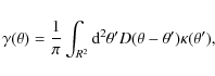
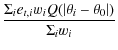
6.1 S-Maps
In Fig. 12
we plot the so-called
S-maps (Schirmer
et al. 2004) for these data. S-maps
are computed as the ratio ![]() where
where
|
|
= | 
|
(10) |
| = | 
|
(11) |
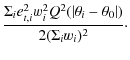
For this calculation the image is considered as a grid of points, et,i are the tangential components of the ellipticities of the lensed galaxies, which are computed by considering the center of each point on the grid, wi is the weight as defined in Eq. (6), and Q is a window function, chosen to be a Gaussian function defined by
|
(12) |
where
![\begin{figure}
\par\includegraphics[width=7.6cm,clip]{12654fg12a.eps}\includegraphics[width=7.6cm,clip]{12654fg12b.eps}
\end{figure}](/articles/aa/full_html/2010/06/aa12654-09/img103.png)
|
Figure 12:
S-maps obtained from the KSB (left panel) and the
Shapelets (right panel) analysis. The levels are
plotted between |
| Open with DEXTER | |
We computed these maps using shear catalogs obtained from both the KSB and shapelet pipelines. In both cases (see Fig. 12), the maps show that the lensing signal is peaked around the BCG, confirming that this is indeed the center of the mass distribution. The mass distribution also appears quite regular, which agrees with what is indicated by the X-ray maps. In Fig. 13, S-map contours are overlaid on the r-band luminosity-weighted density distribution of the red sequence galaxies of Abell 611, selected in Sect. 4, showing that the mass distribution follows that of the red cluster galaxies.
6.2 Aperture densitometry
To trace the mass profile of the cluster, we computed the
![]() -statistic
described in Clowe et al.
(1998) and Fahlman
et al. (1994):
-statistic
described in Clowe et al.
(1998) and Fahlman
et al. (1994):
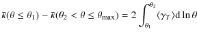
Mass measurements are computed within different apertures of increasing radius using a control annulus far from the center of the distribution (the BCG). Here,
We chose ![]() and
and ![]() ,
which yielded projected masses within
,
which yielded projected masses within ![]() 1500 kpc of
1500 kpc of ![]() and
and ![]() using the KSB and shapelet shear catalogs, respectively.
using the KSB and shapelet shear catalogs, respectively.
Unfortunately we could not extend our analysis farther from the center of the cluster because of the presence of a very bright star in the field making the outer regions unusable.
Since weak lensing is sensitive to the total mass along the line of sight, the observed aperture mass is the sum of the mass of the cluster and any contribution from other, uncorrelated structures along the line of sight. This contribution is assumed to be negligible in the central regions of the cluster, which are much denser, and become more relevant in its outer regions. As discussed by Hoekstra (2001), the effect of this contribution does not introduce any bias, but it does add a source of noise to the lensing mass. Aperture densitometry is more affected by this uncertainty than parametric methods because it is sensitive to the lensing signal at large radii. Nevertheless, for observations of rich clusters at intermediate redshifts, this uncertainty is fairly small because the bulk of the background sources are at much higher redshifts than the cluster.
![\begin{figure}
\par\includegraphics[width=8cm,clip]{12654fg13.eps}
\end{figure}](/articles/aa/full_html/2010/06/aa12654-09/img113.png)
|
Figure 13:
r-band luminosity-weighted density
distribution of red sequence galaxies of Abell 611. The
overlaid contour (black lines) is the S-map (computed and discussed in
Sect. 6.1)
showing the SNR of the shear signal around the cluster obtained from
the shapelet analysis. The levels are plotted between |
| Open with DEXTER | |
6.3 Model fitting
Table 2: Mass values computed for M200 by model fitting using an SIS profile, an NFW profile, and a constrained NFW (MNFW), according to Bullock et al. (2001).
The model-fitting approach for estimating the mass of a cluster consists of assuming a particular analytic mass density profile for which to calculate the expected shear and then fitting the observed shear with the model one by minimizing the log-likelihood function (Schneider et al. 2000):![\begin{displaymath}l_{\gamma}=\sum_{i=1}^{N_{\gamma}}\left[\frac{\vert\epsilon_i...
...ert^2}{
\sigma^2[g(\theta_i)]}+2\ln\sigma[g(\theta_i)]\right],
\end{displaymath}](/articles/aa/full_html/2010/06/aa12654-09/img129.png)
with
In this analysis we assumed both a singular isothermal sphere (SIS) and
a Navarro-Frenk-White (Navarro
et al. 1997) model. In the SIS model the density
profile depends on one parameter, the velocity dispersion ![]() :
:
|
(15) |
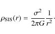
In this profile the shear is found to be related to
|
(16) |
(e.g. Bartelmann & Schneider 2001).
The mass density profile predicted by the Navarro-Frenk-White model
(hereafter NFW) is
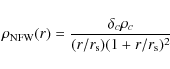
|
(17) |
where
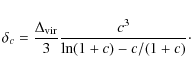
|
(18) |
where
The mass of the halo is
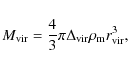
|
(19) |
where
Table 2
shows the best-fit parameters and the mass values derived by model
fitting. The NFW profile was used by keeping both the concentration and
mass as free parameters (marked as NFW) and by using the
relation between
![]() and
and ![]() proposed by Bullock et al.
(2001) (hereafter MNFW):
proposed by Bullock et al.
(2001) (hereafter MNFW): ![]() ,
where
,
where ![]() ,
K=9 and
,
K=9 and ![]() .
.
These values were computed assuming spherical symmetry for the cluster halo. The effect of departures from spherical symmetry (e.g. triaxial halos) on the determination of the total cluster mass have been studied by several authors (e.g. Gavazzi 2005, De Filippis et al. 2005). De Filippis et al. (2005) show that these effects are negligible when the mass is computed at large distances from the cluster center, although they are important at small radii. The same authors tried to recover a three-dimensional reconstruction of Abell 611 through a combined analysis of X-ray and Sunyaev-Zel'dovich observations and conclude that the cluster is approximately spherical, supporting our symmetry assumption.
![\begin{figure}
\par\includegraphics[width=7cm,angle=270]{12654fg14a.ps}\hspace*{2mm}
\includegraphics[width=7cm,angle=270]{12654fg14b.ps}
\end{figure}](/articles/aa/full_html/2010/06/aa12654-09/img147.png)
|
Figure 14:
Results of fitting by an NFW model (dashed lines), a
constrained (M)NFW (solid lines) model (Bullock et al. 2001),
and an SIS profile (dotted lines), with the KSB (left
panel) and shapelet (right panel)
pipeline. Average values of tangential (black) and
radial (red) components of the shear, computed in
logarithmic scale bins, are also plotted. Cluster masses were computed
at r200, estimated to be |
| Open with DEXTER | |
![\begin{figure}
\par\includegraphics[width=8cm,clip]{12654fg15a.eps}\hspace*{1mm}
\includegraphics[width=8cm,clip]{12654fg15b.eps}
\end{figure}](/articles/aa/full_html/2010/06/aa12654-09/img148.png)
|
Figure 15:
The confidence contours for NFW profile are plotted in the ( |
| Open with DEXTER | |
7 Discussion
We conducted a weak lensing analysis of Abell 611 with deep g-band
images from the LBC. Owing to the complexity of the LBC PSF, we decided
to use both the KSB
and shapelet methods to measure galaxy shapes and extract the shear
signal. KSB parametrizes the sources using their weighted quadrupole
moments and is based on a
simplified hypothesis of a nearly circular PSF. In contrast, shapelets
use a decomposition of the images into Gaussian-weighted Hermite
polynomials and does not make any assumption about the best PSF model.
Thanks to the large collecting area of LBT and the wide field of the
LBC, we were able to extract a high number density of ![]() 25 background
galaxies per arcmin2 over a wide field of
25 background
galaxies per arcmin2 over a wide field of ![]() arcmin2 and this allowed us to perform an
accurate weak lensing analysis.
arcmin2 and this allowed us to perform an
accurate weak lensing analysis.
The two shear catalogs, which were derived by the KSB and
shapelet pipelines, were matched and common sources (with a number
density of ![]() 23 galaxies/arcmin2)
were used to estimate mass measurements for Abell 611 by two
different weak lensing techniques: aperture densitometry and a
parametric model fitting. In both approaches we assumed that the BCG
was the center of the mass
distribution, which is supported by S-Maps (see Fig. 12,
Sect. 6.1).
23 galaxies/arcmin2)
were used to estimate mass measurements for Abell 611 by two
different weak lensing techniques: aperture densitometry and a
parametric model fitting. In both approaches we assumed that the BCG
was the center of the mass
distribution, which is supported by S-Maps (see Fig. 12,
Sect. 6.1).
The projected mass values obtained by aperture densitometry
within a radius of ![]() 1500 kpc
are:
1500 kpc
are: ![]() and
and ![]() ,
using KSB and shapelets, respectively. These estimations are
model-independent (Clowe
et al. 1998), but they are affected by large
uncertainties. As discussed in Sect. 14, the contribution
of uncorrelated structures along the line of sight can be source of
noise for aperture measurements, although they can be decreased by
averaging the results for several clusters (Hoekstra
2001) or corrected by using photometric redshifts of the
sources, if available.
,
using KSB and shapelets, respectively. These estimations are
model-independent (Clowe
et al. 1998), but they are affected by large
uncertainties. As discussed in Sect. 14, the contribution
of uncorrelated structures along the line of sight can be source of
noise for aperture measurements, although they can be decreased by
averaging the results for several clusters (Hoekstra
2001) or corrected by using photometric redshifts of the
sources, if available.
Table 2
shows the results of fitting the observed shear with a parametric
model. We assumed both an SIS and an NFW mass density profile. We first
fitted an NFW model by leaving both c and ![]() as free
parameters: as displayed in Fig. 15, the uncertainty
on these
two parameters provided by the fit is high and does not allow a
strong constraint on the concentration. Nevertheless, the best-fit
value
(
as free
parameters: as displayed in Fig. 15, the uncertainty
on these
two parameters provided by the fit is high and does not allow a
strong constraint on the concentration. Nevertheless, the best-fit
value
(![]() )
is in good agreement with the one obtained when the Bullock
et al. (2001) relation is adopted (c =
4.5).
For the NFW fits, the quoted masses are M200,
within the radius r200 where
the density is 200 times the critical density.
The estimated value of r200
for Abell 611 is
)
is in good agreement with the one obtained when the Bullock
et al. (2001) relation is adopted (c =
4.5).
For the NFW fits, the quoted masses are M200,
within the radius r200 where
the density is 200 times the critical density.
The estimated value of r200
for Abell 611 is ![]() 1.5 Mpc
(5.8').
1.5 Mpc
(5.8').
The weak lensing mass measurements obtained from both the KSB
and shapelet shear catalogs agree, within uncertainties: by using an
(M)NFW profile we obtain ![]() and
and ![]() ,
respectively.
The smaller uncertainties of shapelet results show that this method
provides higher accuracy than KSB. Moreover, the goodness of the fits (
,
respectively.
The smaller uncertainties of shapelet results show that this method
provides higher accuracy than KSB. Moreover, the goodness of the fits (![]() )
in Table 2
shows that both shapelets and KSB provide a best fit with higher
probability (Q) by using an NFW mass
density profile rather than an SIS profile.
)
in Table 2
shows that both shapelets and KSB provide a best fit with higher
probability (Q) by using an NFW mass
density profile rather than an SIS profile.
Abell 611 was previously targeted for a weak lensing
study by Dahle (2006),
who used V and I observations
from several facilities to target many clusters (see Dahle et al. 2002 for
more details). They used the KSB (Kaiser
et al. 1995) shear estimator as described in Kaiser (2000) to derive the shear
signal from the images. The mass of the cluster was then derived by
fitting the observed shear with an NFW mass density profile (Navarro et al. 1997). They
assumed a concentration parameter as predicted by Bullock et al. (2001)
and obtained a mass value of ![]() within r180, the radius
within which the density is 180 times the critical density. A
more recent mass estimate of Abell 611 is presented in Pedersen & Dahle (2007), who
use
the data collected in Dahle (2006)
to obtain a value of
within r180, the radius
within which the density is 180 times the critical density. A
more recent mass estimate of Abell 611 is presented in Pedersen & Dahle (2007), who
use
the data collected in Dahle (2006)
to obtain a value of ![]() within r500, the radius
within which the density is 500 times the critical density. In
these papers, the authors extrapolate the NFW profile out to r500
because the data were insufficient to extend this far in projection
from the cluster center. For their work on Abell 611,
within r500, the radius
within which the density is 500 times the critical density. In
these papers, the authors extrapolate the NFW profile out to r500
because the data were insufficient to extend this far in projection
from the cluster center. For their work on Abell 611, ![]() (note
(note
![]() ).
).
Our weak lensing estimates for the mass of Abell 611 agree with the previous results of Dahle (2006) and Pedersen & Dahle (2007), but the depth and the larger area covered by LBC data allowed us to perform a more accurate analysis.
A recent weak lensing analysis of Abell 611 has
recently been done by Okabe
et al. (2009) using Subaru/Suprime-Cam observations
in two filters (i' and V).
The authors use the color (V-i')
information to select the background galaxies for their cluster lensing
analysis, getting a galaxy number density of ![]() 21 galaxies/arcmin2,
with an
21 galaxies/arcmin2,
with an ![]() .
By fitting the mass density profile of the cluster using an NFW model,
they find a mass value
.
By fitting the mass density profile of the cluster using an NFW model,
they find a mass value ![]() and a
and a ![]() (private communication), which are in good agreement with our results.
(private communication), which are in good agreement with our results.
A new mass estimation of Abell 611 was performed by Newman et al. (2009)
over a wide range in cluster-centric distance (from ![]() 3 kpc
to 3.25 Mpc) by combining weak, strong, and kinematic analysis
of the cluster, based on Subaru, HST, and Keck data, respectively. They
found a mass value
3 kpc
to 3.25 Mpc) by combining weak, strong, and kinematic analysis
of the cluster, based on Subaru, HST, and Keck data, respectively. They
found a mass value ![]() with
with ![]() by using an NFW model fitting, in agreement with our results. We note
that such a high value of c cannot be
rejected by our NFW fits, due to the large uncertainties on NFW
parameters (see Table 2
and Fig. 15).
by using an NFW model fitting, in agreement with our results. We note
that such a high value of c cannot be
rejected by our NFW fits, due to the large uncertainties on NFW
parameters (see Table 2
and Fig. 15).
Finally, we also compared the mass values obtained by our weak
lensing analysis to X-ray estimates of M200
available in the literature.
Schmidt & Allen (2007)
analyzed Chandra data of several clusters and modeled their total mass
profile (dark plus luminous matter) using an NFW profile. They found
for Abell 611 a scale radius ![]() Mpc
and a concentration parameter c
= 5.39-1.51+1.60, which
provide a mass value
Mpc
and a concentration parameter c
= 5.39-1.51+1.60, which
provide a mass value
![]() at
at ![]() Mpc,
in agreement, within the uncertainties, with our results. A more recent
X-ray analysis of Chandra observations of Abell 611 has been
performed by Donnarumma
et al. (2010). They obtained a value of
Mpc,
in agreement, within the uncertainties, with our results. A more recent
X-ray analysis of Chandra observations of Abell 611 has been
performed by Donnarumma
et al. (2010). They obtained a value of ![]() at
at ![]() kpc,
with
kpc,
with ![]() kpc
and c
= 4.76-0.78+0.87. Their
projected mass at r200 is
kpc
and c
= 4.76-0.78+0.87. Their
projected mass at r200 is ![]() .
This value agrees, within the statistical uncertainties, with the mass
measured by aperture densitometry, but it is higher than the value
estimated by the parametric model. Additional information on the mass
will be derived from the strong lensing analysis of Abell 611 (Donnarumma et al. 2010).
.
This value agrees, within the statistical uncertainties, with the mass
measured by aperture densitometry, but it is higher than the value
estimated by the parametric model. Additional information on the mass
will be derived from the strong lensing analysis of Abell 611 (Donnarumma et al. 2010).
This work shows that LBT is a powerful instrument for weak lensing studies, but we want to stress that the data analyzed here did not allow us to use the full capabilities of the telescope. The presence of bright saturated stars hampered the use of the whole field of the camera to analyse Abell 611. In addition, the analysis of weak lensing is expected to be improved by using the Red Channel in LBC, which was not yet available during these observations. The present results are nevertheless important to demonstrate the capabilities of LBC for weak lensing, so we plan to extend this analysis to other clusters, this time using the Red Channel.
AcknowledgementsObservations were obtained with the Large Binocular Telescope at Mt. Graham, Arizona, under the Commissioning and Science Demonstration phase of the Blue Channel of the Large Binocular Camera. The LBT is an international collaboration among institutions in the United States, Italy, and Germany. LBT Corporation partners are: The University of Arizona on behalf of the Arizona university system; Istituto Nazionale di Astrofisica, Italy; LBT Beteiligungsgesellschaft, Germany, representing the Max-Planck Society, the Astrophysical Institute Potsdam, and Heidelberg University; The Ohio State University, and The Research Corporation, on behalf of The University of Notre Dame, University of Minnesota, and University of Virginia.This paper makes use of photometric redshifts produced jointly by Terapix and the VVDS team.
Part of the data analysis in this paper was done with the R software (http://www.R-project.org).
We thank the anonymous referee for useful comments and suggestions that improved the presentation of this work. A.R. acknowledges the financial support from contract ASI-COFIS I/016/07/0. L.F., K.K., and M.R. acknowledge the support of the European Commission Programme 6-th framework, Marie Curie Training and Research Network ``DUEL'', contract number MRTN-CT-2006-036133. L.F. is partly supported by the Chinese National Science Foundation Nos. 10878003 & 10778725, 973 Program No. 2007CB 815402, Shanghai Science Foundations and Leading Academic Discipline Project of Shanghai Normal University (DZL805). A.D., S.E., L.M., M.M. acknowledge the financial contribution from contracts ASI-INAF I/023/05/0 and I/088/06/0. SPH is supported by the P2I program, contract number 102759.
References
- Allen, S. W., Schmidt, R. W., Ebeling, H., Fabian, A. C., & van Speybroeck, L. 2004, MNRAS, 353, 457 [NASA ADS] [CrossRef] [Google Scholar]
- Allen, S. W., Rapetti, D. A., Schmidt, R. W., et al. 2008, MNRAS, 383, 879 [NASA ADS] [CrossRef] [Google Scholar]
- Bartelmann, M. 1996, A&A, 313, 697 [NASA ADS] [Google Scholar]
- Bartelmann, M., & Schneider, P. 2001, Phys. Rep., 340, 291 [NASA ADS] [CrossRef] [Google Scholar]
- Bernstein, G. M., & Jarvis, M. 2002, AJ, 123, 583 [NASA ADS] [CrossRef] [Google Scholar]
- Bertin, E., & Arnouts, S. 1996, A&AS, 117, 393 [NASA ADS] [CrossRef] [EDP Sciences] [Google Scholar]
- Bryan, G. L., & Norman, M. L. 1998, ApJ, 495, 80 [NASA ADS] [CrossRef] [Google Scholar]
- Bullock, J. S., Kolatt, T. S., Sigad, Y., et al. 2001, MNRAS, 321, 559 [Google Scholar]
- Clowe, D., & Schneider, P. 2001, A&A, 379, 384 [NASA ADS] [CrossRef] [EDP Sciences] [Google Scholar]
- Clowe, D., & Schneider, P. 2002, A&A, 395, 385 [NASA ADS] [CrossRef] [EDP Sciences] [Google Scholar]
- Clowe, D., Luppino, G. A., Kaiser, N., Henry, J. P., & Gioia, I. M. 1998, ApJ, 497, L61 [NASA ADS] [CrossRef] [Google Scholar]
- Dahle, H. 2006, ApJ, 653, 954 [NASA ADS] [CrossRef] [Google Scholar]
- Dahle, H., Kaiser, N., Irgens, R. J., Lilje, P. B., & Maddox, S. J. 2002, ApJS, 139, 313 [NASA ADS] [CrossRef] [Google Scholar]
- De Filippis, E., Sereno, M., Bautz, M. W., et al. 2005, ApJ, 625, 108 [NASA ADS] [CrossRef] [Google Scholar]
- Donnarumma, A., Ettori, S., Meneghetti, M., et al. 2010, A&A, submitted, [arXiv:1002.1625] [Google Scholar]
- Eke, V. R., Cole, S., Frenk, C. S., et al. 1998, MNRAS, 298, 1145 [NASA ADS] [CrossRef] [Google Scholar]
- Erben, T., Van Waerbeke, L., Bertin, E., Mellier, Y., & Schneider, P. 2001, A&A, 366, 717 [NASA ADS] [CrossRef] [EDP Sciences] [Google Scholar]
- Ettori, S., Morandi, A., Tozzi, P., et al. 2009, A&A, 501, 61 [NASA ADS] [CrossRef] [EDP Sciences] [Google Scholar]
- Evrard, A. E. 1989, ApJ, 341, L71 [NASA ADS] [CrossRef] [Google Scholar]
- Fahlman, G., Kaiser, N., Squires, G., et al. 1994, ApJ, 437, 56 [NASA ADS] [CrossRef] [Google Scholar]
- Gavazzi, R., Mellier, Y., Fort, B., et al. 2004, A&A, 422, 407 [NASA ADS] [CrossRef] [EDP Sciences] [Google Scholar]
- Gavazzi, R. 2005, A&A, 443, 793 [NASA ADS] [CrossRef] [EDP Sciences] [Google Scholar]
- Giallongo, E., Ragazzoni, R., Grazian, A., et al. 2008, A&A, 482, 349 [NASA ADS] [CrossRef] [EDP Sciences] [Google Scholar]
- Henry, J. P. 2000, ApJ, 534, 565 [Google Scholar]
- Hetterscheidt, M., Simon, P., Schirmer, M., et al. 2007, A&A, 468, 859 [NASA ADS] [CrossRef] [EDP Sciences] [Google Scholar]
- Hoekstra, H. 2001, A&A, 370, 743 [NASA ADS] [CrossRef] [EDP Sciences] [Google Scholar]
- Hoekstra, H. 2007, MNRAS, 379, 317 [NASA ADS] [CrossRef] [Google Scholar]
- Hoekstra, H., Franx, M., Kuijken, K., et al. 1998, New Astron. Rev., 42, 137 [NASA ADS] [CrossRef] [Google Scholar]
- Hoekstra, H., Franx, M., & Kuijken, K. 2000, ApJ, 532, 88 [NASA ADS] [CrossRef] [Google Scholar]
- Ilbert, O., Arnouts, S., McCracken, H. J., et al. 2006, A&A, 457, 841 [NASA ADS] [CrossRef] [EDP Sciences] [Google Scholar]
- Kaiser, N. 2000, ApJ, 537, 555 [NASA ADS] [CrossRef] [Google Scholar]
- Kaiser, N., & Squires, G. 1993, ApJ, 404, 441 [NASA ADS] [CrossRef] [Google Scholar]
- Kaiser, N., Squires, G., & Broadhurst, T. 1995, ApJ, 449, 460 [NASA ADS] [CrossRef] [Google Scholar]
- King, L. J., & Schneider, P. 2001, A&A, 369, 1 [NASA ADS] [CrossRef] [EDP Sciences] [Google Scholar]
- Kuijken, K. 2006, A&A, 456, 827 [NASA ADS] [CrossRef] [EDP Sciences] [Google Scholar]
- Luppino, G. A., & Kaiser, N. 1997, ApJ, 475, 20 [NASA ADS] [CrossRef] [Google Scholar]
- Massey, R., & Refregier, A. 2005, MNRAS, 363, 197 [NASA ADS] [CrossRef] [Google Scholar]
- Metzler, C. A., White, M., & Loken, C. 2001, ApJ, 547, 560 [NASA ADS] [CrossRef] [Google Scholar]
- Miller, C. J., Nichol, R. C., Reichart, D., et al. 2005, AJ, 130, 968 [Google Scholar]
- Navarro, J. F., Frenk, C. S., & White, S. D. M. 1997, ApJ, 490, 493 [NASA ADS] [CrossRef] [Google Scholar]
- Newman, A. B., Treu, T., Ellis, R. S., et al. 2009, ApJ, 706, 1078 [NASA ADS] [CrossRef] [Google Scholar]
- Okabe, N., Takada, M., Umetsu, K., Futamase, T., & Smith, G. P. 2009, PASJ, [arXiv:0903.1103] [Google Scholar]
- Paulin-Henriksson, S., Antonuccio-Delogu, V., Haines, C. P., et al. 2007, A&A, 467, 427 [NASA ADS] [CrossRef] [EDP Sciences] [Google Scholar]
- Pedersen, K., & Dahle, H. 2007, ApJ, 667, 26 [NASA ADS] [CrossRef] [Google Scholar]
- Press, W. H., Flannery, B. P., & Teukolsky, S. A. 1986, Numerical recipes. The art of scientific computing, ed. W. H. Press, B. P. Flannery, & S. A. Teukolsky [Google Scholar]
- Radovich, M., Puddu, E., Romano, A., Grado, A., & Getman, F. 2008, A&A, 487, 55 [NASA ADS] [CrossRef] [EDP Sciences] [Google Scholar]
- Refregier, A. 2003, MNRAS, 338, 35 [NASA ADS] [CrossRef] [Google Scholar]
- Schirmer, M., Erben, T., Schneider, P., Wolf, C., & Meisenheimer, K. 2004, A&A, 420, 75 [NASA ADS] [CrossRef] [EDP Sciences] [Google Scholar]
- Schmidt, R. W., & Allen, S. W. 2007, MNRAS, 379, 209 [NASA ADS] [CrossRef] [Google Scholar]
- Schneider, P., King, L., & Erben, T. 2000, A&A, 353, 41 [NASA ADS] [Google Scholar]
- Struble, M. F., & Rood, H. J. 1999, ApJS, 125, 35 [NASA ADS] [CrossRef] [Google Scholar]
- Vikhlinin, A., Kravtsov, A. V., Burenin, R. A., et al. 2009, ApJ, 692, 1060 [NASA ADS] [CrossRef] [Google Scholar]
- Wright, C. O., & Brainerd, T. G. 2000, ApJ, 534, 34 [NASA ADS] [CrossRef] [Google Scholar]
Footnotes
- ... pipeline
![[*]](/icons/foot_motif.png)
- http://lbc.oa-roma.inaf.it
- ...ARP
- Developed by Bertin, http://terapix.iap.fr
- ... IMCAT
- http://www.ifa.hawai.edu/ kaiser/imcat
All Tables
Table 1: Exposure times, limiting magnitudes for point-like sources and zero points (AB) for the observations in each band.
Table 2: Mass values computed for M200 by model fitting using an SIS profile, an NFW profile, and a constrained NFW (MNFW), according to Bullock et al. (2001).
All Figures
|
|
Figure 1:
A three-color image (
|
| Open with DEXTER | |
| In the text | |
|
|
Figure 2: g-band image of the full field of LBC, centered on Abell 611. The box marks the region of 5000 pixels we used for the analysis. |
| Open with DEXTER | |
| In the text | |
|
|
Figure 3:
Magnitude (g) vs. half-light radius ( |
| Open with DEXTER | |
| In the text | |
|
|
Figure 4: The fraction of likely foreground and cluster galaxies (top-panel) and background galaxies (bottom-panel) from the CFHTLS versus magnitude cut in g-band. The dotted vertical line is the lower limit of the magnitude cut adopted to select background galaxies. See Sect. 3 for details. |
| Open with DEXTER | |
| In the text | |
|
|
Figure 5: Color-magnitude plot of the galaxies in the Abell 611 field. Red points are the candidate cluster galaxies selected by the C4 method. Also displayed (solid line) is the results of the biweight regression fit. |
| Open with DEXTER | |
| In the text | |
|
|
Figure 6: Removal of PSF anisotropy in the KSB approach. The observed (top-left), fitted (top-right), and residual (bottom-left) ellipticities of stars for all CCDs. The observed (black points) versus corrected (green points) ellipticities are also shown (bottom-right). |
| Open with DEXTER | |
| In the text | |
|
|
Figure 7:
|
| Open with DEXTER | |
| In the text | |
|
|
Figure 8: Shapelet PSF models interpolated at different positions on each CCD. The distribution of these models corresponds to their actual placement on the CCD mosaic, CCD1 to CCD3 from left to right in the bottom panel and CCD4 in the top. Contours are the representations of PSF shape decomposed by shapelets. The X and Y values correspond to the pixel position. |
| Open with DEXTER | |
| In the text | |
|
|
Figure 9: The star at the position near the center of each CCD is taken as an example to show the residual of PSF model fitting ( left column). The real PSF shape and fitted PSF model are shown in the middle and right columns. |
| Open with DEXTER | |
| In the text | |
|
|
Figure 10: Comparison between the first component of the shear from the shapelet and KSB methods (results with the second components are very similar). |
| Open with DEXTER | |
| In the text | |
|
|
Figure 11:
The plot of the normalized galaxy weight as function of the absolute
first component of ellipticity for KSB measurement. The
applied normalization was |
| Open with DEXTER | |
| In the text | |
|
|
Figure 12:
S-maps obtained from the KSB (left panel) and the
Shapelets (right panel) analysis. The levels are
plotted between |
| Open with DEXTER | |
| In the text | |
|
|
Figure 13:
r-band luminosity-weighted density
distribution of red sequence galaxies of Abell 611. The
overlaid contour (black lines) is the S-map (computed and discussed in
Sect. 6.1)
showing the SNR of the shear signal around the cluster obtained from
the shapelet analysis. The levels are plotted between |
| Open with DEXTER | |
| In the text | |
|
|
Figure 14:
Results of fitting by an NFW model (dashed lines), a
constrained (M)NFW (solid lines) model (Bullock et al. 2001),
and an SIS profile (dotted lines), with the KSB (left
panel) and shapelet (right panel)
pipeline. Average values of tangential (black) and
radial (red) components of the shear, computed in
logarithmic scale bins, are also plotted. Cluster masses were computed
at r200, estimated to be |
| Open with DEXTER | |
| In the text | |
|
|
Figure 15:
The confidence contours for NFW profile are plotted in the ( |
| Open with DEXTER | |
| In the text | |
Copyright ESO 2010
Current usage metrics show cumulative count of Article Views (full-text article views including HTML views, PDF and ePub downloads, according to the available data) and Abstracts Views on Vision4Press platform.
Data correspond to usage on the plateform after 2015. The current usage metrics is available 48-96 hours after online publication and is updated daily on week days.
Initial download of the metrics may take a while.