| Issue |
A&A
Volume 514, May 2010
|
|
|---|---|---|
| Article Number | A35 | |
| Number of page(s) | 25 | |
| Section | Stellar atmospheres | |
| DOI | https://doi.org/10.1051/0004-6361/200911899 | |
| Published online | 07 May 2010 | |
- Top
- Abstract
- 1 Introduction
- 2 Model atmospheres and ...
- 3 Line formation in ...
- 4 The influence of ...
- 5 Simulating line ...
- 6 Towards realistic ...
- 7 CO
Line formation in AGB atmospheres including velocity effects
Molecular line profile variations of long period variables
W. Nowotny1 - S. Höfner2 - B. Aringer1
1 - University of Vienna, Department of Astronomy, Türkenschanzstraße 17, 1180 Wien, Austria
2 - Department of Physics and Astronomy, Division of Astronomy and Space Physics, Uppsala University, Box 515, 75120 Uppsala, SwedenReceived 20 February 2009 / Accepted 19 January 2010
Abstract
Context. Towards the end of the evolutionary stage of the asymptotic giant branch (AGB) the atmospheres of evolved red giants are considerably influenced by radial pulsations of the stellar interiors and developing stellar winds. The resulting complex velocity fields severely affect molecular line profiles (shapes, time-dependent shifts in wavelength, multiple components) observable in near-infrared spectra of long period variables. Time-series high-resolution spectroscopy allows us to probe the atmospheric kinematics and thereby study the mass loss process.
Aims. With the help of model calculations the complex line formation process in AGB atmospheres was explored with the focus on velocity effects. Furthermore, we aimed for atmospheric models which are able to quantitatively reproduce line profile variations found in observed spectra of pulsating late-type giants.
Methods. Models describing pulsation-enhanced dust-driven winds were used to compute synthetic spectra under the assumptions of chemical equilibrium and LTE. For this purpose, we used molecular data from line lists for the considered species and solved the radiative transfer in spherical geometry including the effects of velocity fields. Radial velocities (RV) derived from Doppler-shifted (components of) synthetic line profiles provide information on the gas velocities in the line-forming region of the spectral features. In addition, we made use of radial optical depth distributions to give estimates for the layers where lines are formed and to illustrate the effects of velocities in the line formation process.
Results. Assuming uniform gas velocities for all depth points of an atmospheric model we estimated the conversion factor between gas velocities and measured RVs to p = /RV
/RV  1.2-1.5. On the basis of dynamic model atmospheres and by
applying our spectral synthesis codes we investigated in detail the
finding that various molecular features in AGB spectra
originate at different geometrical depths of the very extended
atmospheres of these stars. We show that the models are able to
quantitatively reproduce the characteristic line profile variations of
lines sampling the deep photosphere (CO
1.2-1.5. On the basis of dynamic model atmospheres and by
applying our spectral synthesis codes we investigated in detail the
finding that various molecular features in AGB spectra
originate at different geometrical depths of the very extended
atmospheres of these stars. We show that the models are able to
quantitatively reproduce the characteristic line profile variations of
lines sampling the deep photosphere (CO  = 3, CN)
of Mira variables and the corresponding discontinuous, S-shaped
RV curve. The global velocity fields (traced by different
features) of typical long-period variables are also realistically
reproduced. Possible reasons for discrepancies concerning other
modelling results (e.g. CO = 2 lines)
are outlined. In addition, we present a model showing
variations of CO =
3 line profiles comparable to observed spectra of semiregular
variables and discuss that the non-occurence of line doubling in these
objects may be due to a density effect.
= 3, CN)
of Mira variables and the corresponding discontinuous, S-shaped
RV curve. The global velocity fields (traced by different
features) of typical long-period variables are also realistically
reproduced. Possible reasons for discrepancies concerning other
modelling results (e.g. CO = 2 lines)
are outlined. In addition, we present a model showing
variations of CO =
3 line profiles comparable to observed spectra of semiregular
variables and discuss that the non-occurence of line doubling in these
objects may be due to a density effect.
Conclusions. The results of our line profile modelling are another indication that the dynamic models studied here are approaching a realistic representation of the outer layers of AGB stars with or without mass loss.Key words: stars: late-type - stars: AGB and post-AGB - stars: atmospheres - infrared: stars - line: profiles - line: formation
1 Introduction
Stars on the asymptotic giant branch (AGB) represent objects of low to intermediate main sequence mass (
0.8-8  )
in a late evolutionary phase. While they exhibit low effective
temperatures (<3500 K), their luminosities can reach
values of up to a few 10
)
in a late evolutionary phase. While they exhibit low effective
temperatures (<3500 K), their luminosities can reach
values of up to a few 10
 at the tip of the AGB, placing them in the upper right corner
of the Hertzsprung-Russell diagram. Compared to the atmospheres of most
other types of stars the outer layers of these evolved red giants have
remarkable properties (see e.g. the review by Gustafsson
& Höfner 2004,
below GH04).
at the tip of the AGB, placing them in the upper right corner
of the Hertzsprung-Russell diagram. Compared to the atmospheres of most
other types of stars the outer layers of these evolved red giants have
remarkable properties (see e.g. the review by Gustafsson
& Höfner 2004,
below GH04). In the cool and very extended atmospheres (extensions of the same order as the radii of the stars; up to a few 100
 ), molecules
can form. Their large number of internal degrees of freedom results in
a plethora of spectral lines. Thus, molecules significantly affect the
spectral appearance of late-type giants at visual and infrared
wavelengths (IR; e.g. Lançon & Wood 2000;
Gautschy-Loidl et al. 2004,
GH04; Aringer et al. 2009).
), molecules
can form. Their large number of internal degrees of freedom results in
a plethora of spectral lines. Thus, molecules significantly affect the
spectral appearance of late-type giants at visual and infrared
wavelengths (IR; e.g. Lançon & Wood 2000;
Gautschy-Loidl et al. 2004,
GH04; Aringer et al. 2009).
On the upper part of the AGB, the stars become instable to strong radial pulsations. This leads to a pronounced variability of the emitted flux with amplitudes of up to several magnitudes in the visual (e.g. Lattanzio & Wood 2004). Since the variations occur on long time scales of a few 10 to several 100 days, pulsating AGB stars are often referred to as long period variables (LPVs). In the past, different types of LPVs were empirically classified according to the regularity of the light change and the visual light amplitude: Mira variables (regular,
 > 2.5
> 2.5 ),
semiregular variables (SRVs, poor regularity, < 2.5), and
irregular variables (irregular, < 1-2). Major
advances in our understanding of the pulsation of AGB stars
were achieved by exploiting the data sets of surveys for microlensing
events (MACHO, OGLE, EROS), which produced a substantial number of
high-quality lightcurves for red variables as a by-product. According
to the pioneering work in this field by Wood et al. (1999) and Wood (2000), and to a
number of subsequent studies (e.g. Lebzelter et al. 2002; Ita
et al. 2004a,b)
it is probably more adequate to characterise LPVs according to their
pulsation mode than to their light change in the visual as it was done
historically. From observational studies during recent years
(see e.g. Lattanzio & Wood 2004) it appears
that stars start to pulsate (as SRVs) in the second/third overtone mode
(corresponding to sequence A in Fig. 1 of Wood 2000) and switch
then to the first overtone mode (sequence B). Light amplitudes
are increasing while the stars evolve and finally become Miras. In this
stadium they pulsate in the fundamental mode (sequence C) and
show highly periodic light changes. Observational evidence for this
evolution scenario was found for LPVs in the globular
cluster 47 Tuc by Lebzelter et al. (2005b) and
Lebzelter & Wood (2005).
),
semiregular variables (SRVs, poor regularity, < 2.5), and
irregular variables (irregular, < 1-2). Major
advances in our understanding of the pulsation of AGB stars
were achieved by exploiting the data sets of surveys for microlensing
events (MACHO, OGLE, EROS), which produced a substantial number of
high-quality lightcurves for red variables as a by-product. According
to the pioneering work in this field by Wood et al. (1999) and Wood (2000), and to a
number of subsequent studies (e.g. Lebzelter et al. 2002; Ita
et al. 2004a,b)
it is probably more adequate to characterise LPVs according to their
pulsation mode than to their light change in the visual as it was done
historically. From observational studies during recent years
(see e.g. Lattanzio & Wood 2004) it appears
that stars start to pulsate (as SRVs) in the second/third overtone mode
(corresponding to sequence A in Fig. 1 of Wood 2000) and switch
then to the first overtone mode (sequence B). Light amplitudes
are increasing while the stars evolve and finally become Miras. In this
stadium they pulsate in the fundamental mode (sequence C) and
show highly periodic light changes. Observational evidence for this
evolution scenario was found for LPVs in the globular
cluster 47 Tuc by Lebzelter et al. (2005b) and
Lebzelter & Wood (2005).
The pulsating stellar interior of an AGB star severely influences the outer layers. The atmospheric structure is periodically modulated, and in the wake of the emerging shock waves dust condensation can take place. Radiation pressure on the newly formed dust grains (at least in the C-rich case, cf. Sect. 2.1) leads to the development of a rather slow (terminal velocities of max. 30 km s-1) but dense stellar wind with high mass loss rates (from a few 10-8 up to 10-4
yr-1;
e.g. Olofsson 2004).
As a consequence of these dynamic processes - pulsation and mass loss - the atmospheres of evolved AGB stars eventually become even more extended than non-pulsating red giants in earlier evolutionary stages. The resulting atmospheric structure strongly deviates from a hydrostatic configuration and shows temporal variations on global and local scales (Sect. 2). The complex, non-monotonic velocity fields with relative macroscopic motions of the order of 10 km s-1 have substantial influence on the shapes of individual spectral lines (Doppler effect). Observational studies have demonstrated that time series high-resolution spectroscopy in the near IR (where AGB stars are bright and well observable) is a valuable tool to study atmospheric kinematics throughout the outer layers of pulsating and mass-losing red giants (e.g. Hinkle et al. 1982, from now on HHR82; or Alvarez et al. 2000). Radial velocities (RV) derived from Doppler-shifts of various spectral lines provide clues on the gas velocities in the line-forming regions of the respective features. A detailed review on studies of line profile variations for AGB stars (observations and modelling) can be found for example in Nowotny (2005, below N05).
In two previous papers (Nowotny et al. 2005a,b, from now on Paper I and Paper II, respectively) we investigated whether observed variations of line profiles can be comprehended with state-of-the-art dynamic model atmospheres. We were able to show that the used models allow to qualitatively reproduce the behaviour of spectral lines originating in different regions of the extended atmospheres. The work presented here can be regarded as an extension of the previous two papers about line profile modelling. The aim is to shed light on the intricate line formation process within the atmospheres of evolved red giants with an emphasis on the velocity effects (Sects. 3-5 and 7.4). In addition, we report on our efforts to achieve realistic models, which are able to reproduce line profile variations and the derived RVs even quantitatively (Sects. 6 and 7).
2 Model atmospheres and spectral synthesis
2.1 General remarks
Modelling the cool and very extended atmospheres of evolved AGB stars remains challenging due to the intricate interaction of different complicated phenomena (convection, pulsation, radiation, molecular and dust formation/absorption, acceleration of winds). Dynamic model atmospheres are constructed to simulate and understand the physical processes (e.g. mass loss) occuring in the outer layers of AGB stars. In particular they are needed if one is interested in reproducing the complex and temporally varying atmospheric structures that form the basis for radiative transfer calculations, which allows us to simulate observational results (spectra, photometry, etc.).
For our line profile modelling we used dynamic model atmospheres as described in detail by Höfner et al. (2003; DMA3), Gautschy-Loidl et al. (2004; DMA4), N05 or Papers I and II. These models represent the scenario of pulsation-enhanced dust-driven winds (cf. Sects. 4.7 and 4.8 of GH04). They provide a consistent and realistic description from the deep and dust-free photosphere (dominated by the pulsation of the stellar interior) out to the dust-forming layers and beyond to the stellar wind region at the inner circumstellar envelope (characterised by the cool, steady outflow). This is accomplished by a combined and self-consistent solution of hydrodynamics, frequency-dependent radiative transfer and a detailed time-dependent treatment of dust formation and evolution.
As a result of deep-reaching convection (dredge-up), nucleo-synthesis products can be mixed up from the stellar interior of AGB stars, resulting in a metamorphosis of the molecular chemistry of the whole atmosphere (e.g. Busso et al. 1999; Herwig 2005). The most important product of all the nuclearly processed material mixed up is carbon 12C. As a consequence, the stars can turn from oxygen-rich (C/O < 1) to carbon-rich (C/O > 1) during the late AGB phase. The resulting so-called carbon stars (C stars) can be found close to the tip of the AGB in observed colour-magnitude diagrams (e.g. Nowotny et al. 2003a). The drastic change of the atmospheric chemical composition is not only relevant for the observable spectral type of the star (changing from M to C), it is also crucial for the formation of circumstellar dust.
Observational studies revealed a rich mineralogy in the dusty outflows of O-rich objects (e.g. Molster & Waters 2003, and references therein). Unfortunately, the dust formation process is theoretically not fully understood. Many physical and chemical details of the process are still not clear, which would be necessary for a fully consistent numerical treatment. In addition to the lack of a grain formation theory, there is an ongoing debate concerning the underlying physics of the driving mechanism (Woitke 2006b, 2007; Höfner 2007; Höfner & Andersen 2007). A potential solution was recently suggested by Höfner (2008).
Things are quite different for C-rich stars, where we find a rather simple composition of the circumstellar dust. A very limited variety of dust species were identified by their spectral features (e.g. Molster & Waters 2003), as for example SiC (prominent feature at
11  m)
or MgS (broad emission band around 30 m). The most
important species is amorphous carbon dust, though. Not producing any
distinctive spectral feature, grains of carbon dust represent the
dominating condensate and play a crucial role from the dynamic point of
view (mass loss process). Amorphous carbon fulfills the relevant
criteria for a catalyst of dust-driven winds: (i) made up of
abundant elements; (ii) simple and efficient formation
process; (iii) refractory, i.e. stable at high
temperatures (1500 K);
(iv) large radiative cross section around 1 m in order
to absorb momentum. Moreover, the formation and evolution of amorphous
carbon dust grains can be treated numerically in a consistent way by
using moment equations as described in Gail & Sedlmayr (1988) and Gauger
et al. (1990).
As a consequence of this, atmospheric models for
C-rich AGB stars with dusty outflows were quite successfully
calculated and applied in the past by different groups
(see the overviews given by Woitke 2003; or Höfner
et al. 2005),
among them the models used in this work.
m)
or MgS (broad emission band around 30 m). The most
important species is amorphous carbon dust, though. Not producing any
distinctive spectral feature, grains of carbon dust represent the
dominating condensate and play a crucial role from the dynamic point of
view (mass loss process). Amorphous carbon fulfills the relevant
criteria for a catalyst of dust-driven winds: (i) made up of
abundant elements; (ii) simple and efficient formation
process; (iii) refractory, i.e. stable at high
temperatures (1500 K);
(iv) large radiative cross section around 1 m in order
to absorb momentum. Moreover, the formation and evolution of amorphous
carbon dust grains can be treated numerically in a consistent way by
using moment equations as described in Gail & Sedlmayr (1988) and Gauger
et al. (1990).
As a consequence of this, atmospheric models for
C-rich AGB stars with dusty outflows were quite successfully
calculated and applied in the past by different groups
(see the overviews given by Woitke 2003; or Höfner
et al. 2005),
among them the models used in this work.
2.2 Models for atmospheres and winds
Table 1: Characteristics of the dynamic atmospheric models for pulsating, C-rich AGB stars used for the modelling (for a detailed description see text and DMA3).
Following the previous remarks, we concentrated in this study on model atmospheres for C-type LPVs for our line profile modelling, because these models contain a more consistent prescription of dust formation
![[*]](/icons/foot_motif.png) . However, the velocity
effects on line profiles are of general relevance, and a comparison
with observational results of stars with other spectral types
(e.g.
. However, the velocity
effects on line profiles are of general relevance, and a comparison
with observational results of stars with other spectral types
(e.g.  Cyg)
should be justified. This is especially the case for CO lines
because of the characteristic properties of this molecule
(e.g. Sect. 2.2 in Paper I). Table 1 lists the
parameters and the resulting wind properties of the dynamic models used
in this work.
Cyg)
should be justified. This is especially the case for CO lines
because of the characteristic properties of this molecule
(e.g. Sect. 2.2 in Paper I). Table 1 lists the
parameters and the resulting wind properties of the dynamic models used
in this work.
The starting point for the calculation is a hydrostatic initial model, which is very similar to classical model atmospheres (Fig. 1 in DMA3), as for example those calculated with the MARCS-Code (Gustafsson et al. 2008). These initial models are characterised by a set of parameters as listed in the first part of Table 1. They are dust-free and rather compact in comparison with fully developped dynamical structures (e.g. Fig. 4). The effects of pulsation of the stellar interior are then simulated by a variable inner boundary
This so-called piston moves sinusoidally with a period P and a velocity amplitude .
Assuming a constant radiative flux at the inner boundary, the
luminosity
.
Assuming a constant radiative flux at the inner boundary, the
luminosity
 varies like
 for the models presented in DMA3. The assumptions for the
inner boundary were slightly adapted for the latest generation of
models as discussed in DMA4: an additional free
parameter
for the models presented in DMA3. The assumptions for the
inner boundary were slightly adapted for the latest generation of
models as discussed in DMA4: an additional free
parameter  was introduced so that the luminosity at the inner boundary
varies like
was introduced so that the luminosity at the inner boundary
varies like
where and
and  are the values at the inner boundary of the hydrostatic initial model ( =
  ,
by definition, and
,
by definition, and  corresponds to the previously used case of constant flux at the inner
boundary). The luminosity variation
amplitude of the model can be adjusted thereby independent of the
mechanical energy input by the piston. This allows us to tune the
bolometric amplitudes
corresponds to the previously used case of constant flux at the inner
boundary). The luminosity variation
amplitude of the model can be adjusted thereby independent of the
mechanical energy input by the piston. This allows us to tune the
bolometric amplitudes
 to resemble more closely the values derived from observational studies.
Figure 3a
shows the variability of the luminosity L
of one dynamic model as an example.
to resemble more closely the values derived from observational studies.
Figure 3a
shows the variability of the luminosity L
of one dynamic model as an example.
As described in detail in DMA3, the models can be divided into two sub-groups according to their dynamical behaviour:
-

- pulsating model atmospheres where no dust forms;
-
- models developing pulsation-enhanced dust-driven winds.
![\begin{figure}
\par\includegraphics[width=8.8cm,clip]{11899fig01.ps}
\end{figure}](/articles/aa/full_html/2010/06/aa11899-09/Timg55.png)
Figure 1: Movement of mass shells with time at different depths of the dust-free model W, which exhibits no mass loss and shows a strictly periodic behaviour for all layers. Note the different scales on the radius-ordinates compared to Fig. 2. The shown trajectories represent the points of the adaptive grid at a selected instance of time (higher density of points at the location of shocks) and their evolution with time (cf. the caption of Fig. 2 in DMA3 for further explanations).
Open with DEXTER The atmospheres of LPVs become qualitatively different with the occurence of dust and the development of a stellar wind. The other models listed in Table 1, namely models S and M, represent examples for this second type of dynamic model atmospheres. Again, shock waves are triggered by the pulsating stellar interior and propagate outwards. The difference arises because efficient dust formation can take place in the wake of the shock waves (post-shock regions with strongly enhanced densities at low temperatures). Radiation pressure on the newly formed dust grains results in an outflow of the outer atmospheric layers. This behaviour is demonstrated in Fig. 2, which shows the characteristic pattern of the moving mass layers with model M as an example. While the models without mass loss stay rather compact compared to the hydrostatic initial model (Fig. 3), the models that develop a wind are inflated by it and become much more extended than the corresponding initial model. Numerically, a transmitting outer boundary - allowing outflow; fixed at 20-30
 -
is used for the latter type of dynamic model atmospheres. Spatial
structures of model M are shown in Fig. 4,
demonstrating the strong influence of dust formation on the atmospheric
extension. The models S and M exhibit quite a
moderate dust formation process, which leads to a smooth transistion of
the velocity field from the pulsating inner layers to the steady
outflow of the outer layers (see the velocity structure plots
in Fig. 9
of Paper I and Fig. 4 in
this work). In contrast, the model applied in
Sect. 6.1 of Paper II is a representative of a group
of models with a more extreme dust formation. Not every emerging shock
wave leads to the formation of dust grains (cf. Fig. 20
in DMA3) and the velocity field in the dust-forming region may
look very different for similar phases of different pulsation periods.
Pronounced dust shells arise from time to time and propagate outwards
(see the structure plot in Fig. 10
of Paper II).
-
is used for the latter type of dynamic model atmospheres. Spatial
structures of model M are shown in Fig. 4,
demonstrating the strong influence of dust formation on the atmospheric
extension. The models S and M exhibit quite a
moderate dust formation process, which leads to a smooth transistion of
the velocity field from the pulsating inner layers to the steady
outflow of the outer layers (see the velocity structure plots
in Fig. 9
of Paper I and Fig. 4 in
this work). In contrast, the model applied in
Sect. 6.1 of Paper II is a representative of a group
of models with a more extreme dust formation. Not every emerging shock
wave leads to the formation of dust grains (cf. Fig. 20
in DMA3) and the velocity field in the dust-forming region may
look very different for similar phases of different pulsation periods.
Pronounced dust shells arise from time to time and propagate outwards
(see the structure plot in Fig. 10
of Paper II). ![\begin{figure}
\par\includegraphics[width=8.8cm,clip]{11899fig02.eps}
\end{figure}](/articles/aa/full_html/2010/06/aa11899-09/Timg56.png)
Figure 2: Same plot as Fig. 1 for model M, representing the scenario of a pulsation-enhanced dust-driven wind. The plot illustrates the different regions within the atmosphere of a typical mass-losing LPV. The innermost, dust-free layers below
2
are subject to strictly regular motions caused by the pulsating
interior (shock fronts). The dust-forming region (colour-coded is the
degree of dust condensation  )
at 2-3
where the stellar wind is triggered represents dynamically a transition
region with moderate velocities, not necessarily periodic.
A continuous outflow is found from 4
outwards, where the dust-driven wind is decisive from the dynamic point
of view.
)
at 2-3
where the stellar wind is triggered represents dynamically a transition
region with moderate velocities, not necessarily periodic.
A continuous outflow is found from 4
outwards, where the dust-driven wind is decisive from the dynamic point
of view.
Open with DEXTER We refer to Höfner et al. (2003) for more details about the numerical methods and the atmospheric models.
![\begin{figure}
\par\includegraphics[width=15cm,clip]{11899fig03.ps}
\end{figure}](/articles/aa/full_html/2010/06/aa11899-09/Timg57.png)
Figure 3: Characteristic properties of model W. Plotted in panel a) is the bolometric lightcurve resulting from the variable inner boundary (piston), diamonds mark instances of time for which snapshots of the atmospheric structure were stored by the radiation-hydrodynamics code. Denoted are selected phases for which line profiles are presented in Fig. 20. Other panels: atmospheric structures of the initial hydrostatic model (thick black line) and selected phases
 of the dynamic calculation (colour-coded in the same way as the phase
labels of panel a)). Plotted are gas
temperature b), gas density
c), and gas velocities d). Note
that this is a dust-free model and the degree of condensation of carbon
into dust is = 0
for every depth point at each instance of time.
of the dynamic calculation (colour-coded in the same way as the phase
labels of panel a)). Plotted are gas
temperature b), gas density
c), and gas velocities d). Note
that this is a dust-free model and the degree of condensation of carbon
into dust is = 0
for every depth point at each instance of time.
Open with DEXTER ![\begin{figure}
\par\includegraphics[width=15cm,clip]{11899fig04.ps}
\end{figure}](/articles/aa/full_html/2010/06/aa11899-09/Timg58.png)
Figure 4: Characteristic properties of model M. Radial structures of the initial hydrostatic model (thick black) and selected phases of the dynamic model atmosphere during one pulsation cycle (
= 0.0-
1.0). Plotted are gas temperatures a),
gas densities b), gas velocities
c), and degrees of condensation of carbon into dust
d). Panel b) demonstrates the
larger extension compared to the hydrostatic initial model and the
local density variations.
Open with DEXTER 2.3 The specific models used
Model S was already used extensively in the previous Papers I and II to study line profile variations. Its parameters (listed in Table 1) were chosen to resemble the Mira S Cep, as this is the only C-type Mira with an extensive time series of high-resolution spectroscopy and derived RVs (Fig. 17). Table 1 of Paper II lists properties for this object as compiled from the literature for comparison. Model S should not be taken as a specific fit for S Cep, though. A discussion of the difficulties when relating dynamic model atmospheres to certain objects can be found in Sect. 3 of Paper II (or Sect. 2.1.4 in N05). However, there is evidence that the model reproduces the outer layers of this star reasonably well. There are some properties listed in the mentioned tables which can be compared directly and agree to some extent (e.g. L, P,
 ,
,
 ). In addition,
low-resolution synthetic spectra in the visual and IR computed
on the basis of model S resemble observed
spectra (ISO, KAO) of S Cep fairly well as
it was shown by Gautschy-Loidl et al. (2004; their
Sect. 5.1).
). In addition,
low-resolution synthetic spectra in the visual and IR computed
on the basis of model S resemble observed
spectra (ISO, KAO) of S Cep fairly well as
it was shown by Gautschy-Loidl et al. (2004; their
Sect. 5.1).
Model M was the (so far) last model of a small parameter study we carried out subsequent to Papers I and II. The intention was not to find a model fitting a certain target of observations better, but to change the model parameters in order to reproduce one particular observational aspect: namely the velocity variations in the inner, dust-free photosphere resulting in a rather uniform RV curve for CO
=
3 lines in spectra of Miras as discussed in Sect. 6.1 and shown
in Fig. 14.
The comparison of the global velocity field of this model M
with observational results in Sect. 6.2 is
still done on a qualitative basis, though. Confronting
RV measurements (Fig. 17) with
the corresponding synthetic values (Fig. 18) provides
some general information of how realistic the velocity structures of
the model are. However, a direct and quantitative comparison
of stellar and model parameters is not feasible at the moment due to
limitations on the observational side (very small number of
stars observed extensively, often only rough estimates for properties
of targets) as well as on the modelling side (only C-rich
models, laborious process to get a RV diagramm as
Fig. 18)
as discussed in Sect. 6.2.
While investigating synthetic CO
= 3 line
profile variations based on a few dynamical models available at that
time, we found model W reproducing the observed behaviour of
SRVs (Sect. 7.1)
with similarities to W Hya (increased  RV).
In Sect. 7.3
we will make a comparison of observational and modelling results only
for this very selected aspect. Relating model W (C-rich
chemistry) and the M-type LPV W Hya to constrain the
parameters of this star is even less possible than for the before
mentioned case of model M, and was not intended.
RV).
In Sect. 7.3
we will make a comparison of observational and modelling results only
for this very selected aspect. Relating model W (C-rich
chemistry) and the M-type LPV W Hya to constrain the
parameters of this star is even less possible than for the before
mentioned case of model M, and was not intended.
2.4 Calculating synthetic line profiles
For the spectral synthesis we followed the numerical approach as described in detail in N05 (Sect. 2.2) and also in Papers I and II. The modelling procedure of dynamic model atmospheres (see DMA3) yields some immediate results, like mass loss rates
,
terminal velocities of the winds  ,
or degrees of dust condensation in the outflows .
In addition, it provides snapshots of the
time-dependent atmospheric structure (
,
or degrees of dust condensation in the outflows .
In addition, it provides snapshots of the
time-dependent atmospheric structure ( , T, p,
u, etc.) at several instances of
time (e.g. Figs. 3
and 4).
These represent the starting point for the aspired spectral synthesis,
accomplished in a two-step process as described below.
, T, p,
u, etc.) at several instances of
time (e.g. Figs. 3
and 4).
These represent the starting point for the aspired spectral synthesis,
accomplished in a two-step process as described below.
The first step, calculating opacities based on a given atmospheric structure, was accomplished with the COMA code, a description of which can be found in Aringer (2000), Gautschy-Loidl (2001), or N05. Informations on recent updates and the latest version can be found in Gorfer (2005), Lederer & Aringer (2009), Aringer et al. (2009). Element abundances for the spectral synthesis were used in consistency with the hydrodynamic models of solar composition. We adopted the values from Anders & Grevesse (1989), except for C, N and O where we took the data from Grevesse & Sauval (1994). This agrees with our previous work (e.g. Aringer et al. 1999, 2009) and results in
 0.02.
Subsequently, the carbon abundance was increased according to
the C/O of the models. Abundances and ionisations of various
atoms and formed molecules for all layers of the atmospheric model were
calculated with equilibrium chemistry routines
(for a detailed discussion and an extensive list of
references we refer to Lederer & Aringer 2009). The
depletion of carbon in the gas phase due to consumption by dust grain
formation is also taken into account by the COMA code.
Examples for the resulting partial pressures can be found in
Fig. 5.
Subsequently, opacities for every radial depth point and the chosen
wavelength grid were computed. Several opacity sources were considered,
the most important one being the molecules for which the line profiles
are to be studied. Their contribution to the opacities were computed by
using line lists and under the following assumptions:
(i) conditions of LTE;
(ii) a microturbulence velocity of
0.02.
Subsequently, the carbon abundance was increased according to
the C/O of the models. Abundances and ionisations of various
atoms and formed molecules for all layers of the atmospheric model were
calculated with equilibrium chemistry routines
(for a detailed discussion and an extensive list of
references we refer to Lederer & Aringer 2009). The
depletion of carbon in the gas phase due to consumption by dust grain
formation is also taken into account by the COMA code.
Examples for the resulting partial pressures can be found in
Fig. 5.
Subsequently, opacities for every radial depth point and the chosen
wavelength grid were computed. Several opacity sources were considered,
the most important one being the molecules for which the line profiles
are to be studied. Their contribution to the opacities were computed by
using line lists and under the following assumptions:
(i) conditions of LTE;
(ii) a microturbulence velocity of  = 2.5 km s-1;
and (iii) line shapes described by Doppler profiles. Assuming
LTE conditions, level populations can be computed from
Boltzmann distributions at the corresponding gas temperature T.
The opacity
= 2.5 km s-1;
and (iii) line shapes described by Doppler profiles. Assuming
LTE conditions, level populations can be computed from
Boltzmann distributions at the corresponding gas temperature T.
The opacity
 at a given frequency
  for a certain transition from state m to
state n can then be written as
for a certain transition from state m to
state n can then be written as
with the number density of relevant particles N, the charge e and mass me of the electron, the speed of light c, the Boltzmann constant k, and the energy of the respective radiation. The partition function Q(T)
is the weighted sum of all possible states. E0 represents
the excitation energy of the level m (from
ground state) and gf is the product of the
statistical weight g(m)
of the level times the oscillator strength f(m,n)
of the transition. Line lists usually contain frequencies
of the respective radiation. The partition function Q(T)
is the weighted sum of all possible states. E0 represents
the excitation energy of the level m (from
ground state) and gf is the product of the
statistical weight g(m)
of the level times the oscillator strength f(m,n)
of the transition. Line lists usually contain frequencies  (or in practice wavenumbers), excitation energies E0,
and gf values together with informations
for line identification. In order to reproduce the line shapes
in a realistic way, a broadening function
(or in practice wavenumbers), excitation energies E0,
and gf values together with informations
for line identification. In order to reproduce the line shapes
in a realistic way, a broadening function
 for the line profile was introduced with
(4)
Only the effects of thermal broadening (first term in Eq. (6)) and the non-thermal contribution of microturbulent velocities (second term in Eq. (6)) are taken into account by COMA, whereas other effects (e.g. natural and pressure broadening, macroturbulence) are neglected. We refer to Sect. 2.2.2 of N05 for details. The resulting Doppler profiles can be described by a (Gaussian) broadening function
(5)
with a Doppler width given by
where is the gas constant, the
molecular weight, and
the microturbulent velocity. An updated set of references for
the line lists of all molecular species used by the current version of
COMA can be found in Lederer & Aringer (2009).
In this work we made use of the list of Goorvitch &
Chackerian (1994)
for CO and the CN line list of Jørgensen & Larsson (1990). We utilised
the same molecular lines as in Papers I and II, their
respective properties are summarised in Table 2.
In addition, molecules affecting the spectra
pseudo-continuously (mainly C2H2)
were considered by an opacity of constant value for the considered
spectral range (cf. Sect. 5.1 in Paper I
or N05). Furthermore, continuum absorption coefficients are
determined by COMA (Lederer & Aringer 2009)
as well as the opacity due to dust grains of amorphous carbon.
For the latter we used the data of Rouleau & Martin (1991;
set AC) and computed the resulting dust absorption under the assumption of
the small particle limit of the Mie theory (grain sizes much
smaller than relevant wavelengths
is the gas constant, the
molecular weight, and
the microturbulent velocity. An updated set of references for
the line lists of all molecular species used by the current version of
COMA can be found in Lederer & Aringer (2009).
In this work we made use of the list of Goorvitch &
Chackerian (1994)
for CO and the CN line list of Jørgensen & Larsson (1990). We utilised
the same molecular lines as in Papers I and II, their
respective properties are summarised in Table 2.
In addition, molecules affecting the spectra
pseudo-continuously (mainly C2H2)
were considered by an opacity of constant value for the considered
spectral range (cf. Sect. 5.1 in Paper I
or N05). Furthermore, continuum absorption coefficients are
determined by COMA (Lederer & Aringer 2009)
as well as the opacity due to dust grains of amorphous carbon.
For the latter we used the data of Rouleau & Martin (1991;
set AC) and computed the resulting dust absorption under the assumption of
the small particle limit of the Mie theory (grain sizes much
smaller than relevant wavelengths  opacities proportional to the total amount of condensed material, but
independent of grain size distribution; cf. DMA3, Höfner
et al. 1992).
opacities proportional to the total amount of condensed material, but
independent of grain size distribution; cf. DMA3, Höfner
et al. 1992).
In the second step of the spectral synthesis, the previously calculated data array of opacities
 for all depth and wavelengths points was utilised to solve the
radiative transfer (RT). As the thickness of the
line-forming region in AGB atmospheres is large compared to
the stellar radii, it is necessary to treat the RT in
spherical geometry. In addition, the complex velocity fields
(pattern of outflow and infall as for example shown in Fig. 4) in
AGB atmospheres severely affect the line shapes in the
resulting spectra (observed or synthetic, e.g. Fig. 12),
and it is essential to include the influence of relative macroscopic
velocities in this step of the spectral synthesis. Thus, a code for
solving spherical RT, which takes into account velocity
effects, is used to model line profiles and their variations.
The RT code used in this work (Windsteig 1998) follows the
numerical algorithm described in Yorke (1988).
for all depth and wavelengths points was utilised to solve the
radiative transfer (RT). As the thickness of the
line-forming region in AGB atmospheres is large compared to
the stellar radii, it is necessary to treat the RT in
spherical geometry. In addition, the complex velocity fields
(pattern of outflow and infall as for example shown in Fig. 4) in
AGB atmospheres severely affect the line shapes in the
resulting spectra (observed or synthetic, e.g. Fig. 12),
and it is essential to include the influence of relative macroscopic
velocities in this step of the spectral synthesis. Thus, a code for
solving spherical RT, which takes into account velocity
effects, is used to model line profiles and their variations.
The RT code used in this work (Windsteig 1998) follows the
numerical algorithm described in Yorke (1988).
It is necessary to choose spectral resolutions that are high enough to sample individual spectral lines with a sufficient number of wavelength points. This is especially important for synthesising the often quite complex line profiles for stars with pronounced atmospheric dynamics, like those that are the topic of this work. Therefore, all spectra are calculated with an extremely high resolution of R =
 =
300 000 and were then rebinned to R =
70 000 for comparison with observed FTS spectra.
Furthermore, the synthetic spectra shown below were normalised relative
to a computation with only the continuous opacity taken into
account (F/
=
300 000 and were then rebinned to R =
70 000 for comparison with observed FTS spectra.
Furthermore, the synthetic spectra shown below were normalised relative
to a computation with only the continuous opacity taken into
account (F/
 ).
). Table 2: Different molecular features and the properties of the specific lines used for the line profile modelling here (and in Papers I and II).
Our aim is to infer information about atmospheric velocity fields from shifts in the wavelength of (components of) spectral lines. For this purpose, RVs were calculated by using the rest wavelength of the respective line and the formula for Doppler shift. For an easy comparison of our modelling results with observations, we adopted the naming convention for velocities of observational studies (positive for material moving away from the observer and negative for matter moving towards the observer). Thus, outflow from the star results in blue-shifted lines and negative RVs, while infalling matter revealed by red-shifted lines leads to positive RVs. In general, the RVs resulting from observations were combined into one composite lightcycle (
 = 0.0-1.0)
and then plotted repeatedly for better illustration
(e.g. Fig. 14).
For the modelling we computed spectra and derived RVs throughout one
pulsation period (
= 0.0-1.0)
and replicate the values beyond this interval
(e.g. Fig. 15).
= 0.0-1.0)
and then plotted repeatedly for better illustration
(e.g. Fig. 14).
For the modelling we computed spectra and derived RVs throughout one
pulsation period (
= 0.0-1.0)
and replicate the values beyond this interval
(e.g. Fig. 15).
Following the convention of Papers I and II, bolometric phases
within the lightcycle in luminosity (Fig. 3a) will be
used throughout this work to characterise the modelling results
(atmospheric structures, synthetic spectra, derived RVs, etc.) with
numbers written in italics for a clear distinction
from the visual phases
,
which are usually used to denote observational results (with = 0
corresponding to phases of maximum light in the visual).
For a discussion of the relation between the two
types of phase informations, namely
and
,
we refer to Appendix A.
Throughout this work (e.g. the lower panel of Fig. 6 and all similar plots in the following), the radial optical depth
 is computed by radially integrating inwards
for a given wavelength point
is computed by radially integrating inwards
for a given wavelength point
and is then plotted with dotted lines. For the opacities ,
all relevant sources (continuous, molecular/atomic, dust) are
included. If velocity effects are taken into account, optical
depths are calculated with the opacities at all depth points
Doppler-shifted according to the corresponding gas velocity there and
then plotted with solid lines. The optical depth of
,
all relevant sources (continuous, molecular/atomic, dust) are
included. If velocity effects are taken into account, optical
depths are calculated with the opacities at all depth points
Doppler-shifted according to the corresponding gas velocity there and
then plotted with solid lines. The optical depth of
 1
provides clues on the approximate location of atmospheric layers where
radiation of a certain frequency
(or the corresponding wavelength
1
provides clues on the approximate location of atmospheric layers where
radiation of a certain frequency
(or the corresponding wavelength  )
originates.
)
originates.
3 Line formation in the extended atmospheres of evolved red giant stars
This section is concerned with the fact that different molecular spectral features visible in spectra of AGB stars originate at different atmospheric depths and the examination of this with numerical methods.
Typical main sequence stars exhibit relatively compact photospheres, and the radiation in different wavelengths originates at roughly the same geometrical atmospheric depths with a rather well defined temperature (e.g. Sect. 4.3.1 in GH04). For example, the relative thickness of the flux-forming region where the spectrum is produced in our Sun amounts to
 4
4  10-4
(cf. N05). The often used parameter effective
temperature
10-4
(cf. N05). The often used parameter effective
temperature
 represents a mean temperature in the layers of the thin photosphere,
from where almost all photons can escape.
represents a mean temperature in the layers of the thin photosphere,
from where almost all photons can escape. ![\begin{figure}
\par\includegraphics[width=8.8cm,clip]{11899fig05.ps}
\end{figure}](/articles/aa/full_html/2010/06/aa11899-09/Timg88.png)
Figure 5: Upper panel: atmospheric structure of model S for the phase
=
0.0. Gas velocities
are overplotted for illustration purposes (shock fronts). Compare
Figs. 1
and 9
in Paper I to get an idea of the temporal variations and also
for the scale of the gas velocities. The dotted line marks the border
between the actual model and the extension towards the interior for the
sake of optical depth (see text). Lower panel:
the total gas pressure together with the corresponding partial
pressures of selected molecules for this phase if chemical equilibrium
is assumed. Shown is only a subset of all molecular species considered
by COMA, which are CO, CN, C2, CH, C3,
C2H2, and HCN.
Open with DEXTER In contrast, estimating the atmospheric extensions
 in the case of AGB stars is much more difficult. The outer
boundaries of these objects are hard to define (as discussed
by GH04 in their Sect. 4.1) due to the shallow density
gradients related to the low surface gravities
in the case of AGB stars is much more difficult. The outer
boundaries of these objects are hard to define (as discussed
by GH04 in their Sect. 4.1) due to the shallow density
gradients related to the low surface gravities  ,
intensified by the dynamic processes of pulsation and mass loss.
GH04 give estimates of 0.1-0.5 for the
parameter
/.
For the dynamic models used here (Sect. 2.2), one could
for example consider the region of dust formation at 2 ,
where the onset of the stellar wind takes place
(cf. Fig. 4)
as an outer boundary of the atmosphere. This results in / 1.
Whatever value one adopts, it is clear that the thickness of
an AGB atmosphere is of the same order as the stellar radius,
which is quite different from normal main sequence stars. With these
extremely extended atmospheres, the wavelength-dependent geometrical
radius can vary by a few 100
(equivalent to a few AU) or more. Also the
related gas temperatures can cover a wide range from 5000 K
down to a few hundred Kelvin (N05).
,
intensified by the dynamic processes of pulsation and mass loss.
GH04 give estimates of 0.1-0.5 for the
parameter
/.
For the dynamic models used here (Sect. 2.2), one could
for example consider the region of dust formation at 2 ,
where the onset of the stellar wind takes place
(cf. Fig. 4)
as an outer boundary of the atmosphere. This results in / 1.
Whatever value one adopts, it is clear that the thickness of
an AGB atmosphere is of the same order as the stellar radius,
which is quite different from normal main sequence stars. With these
extremely extended atmospheres, the wavelength-dependent geometrical
radius can vary by a few 100
(equivalent to a few AU) or more. Also the
related gas temperatures can cover a wide range from 5000 K
down to a few hundred Kelvin (N05). In general, molecular lines do not originate in a well-defined and narrow region, but are formed over a more or less wide range in radius. Nevertheless, there have been attempts to constrain the approximative line forming region in radius and temperature for different molecular features with similar dynamical model atmospheres as used here. The results - which should be regarded as rough estimates rather than definite borders, though - are compiled e.g. in Table 1.2 of N05. There are only a few molecular bands (e.g. CN or C2), which are solely formed in the deep, warm layers of the photosphere. Most of the strong features (e.g. H2O, HCN, C2H2) originate in the cool, upper layers of the atmosphere because of the small dissociation energies of the (polyatomic) molecules in combination with the high gf values. It is interesting that there are examples for bands formed in a relatively narrow region, as e.g. the ones of C3, which is due to the interplay between molecular formation and dissociation probabilities (Gautschy-Loidl 2001, Fig. 5). The special role of CO and the corresponding features will be discussed in detail below. To sum this up, the emerging spectrum (across the whole spectral range from the visual to the IR) of an AGB star is formed over a large radial range with diverse physical conditions, which is quite different from the scenario for the Sun as sketched above.
Moreover, not only spectral features of different molecules originate at varying radial atmospheric depths, but also different lines of the same molecular species can show this effect. This is especially pronounced in the case of CO lines and will be investigated below on the basis of one (arbitrarily chosen) phase of model S. The upper panel of Fig. 5 shows the corresponding atmospheric structure
at the phase = 0.0.
There are a few factors that are decisive for the line intensities and for the locations (r,
 )
of the line forming regions of molecular features in
AGB atmospheres:
)
of the line forming regions of molecular features in
AGB atmospheres: - i.
- the atmospheric structure itself (r-T-p);
- ii.
- the relative abundance (i.e. partial pressure) of the considered molecular species at certain depth points within the atmosphere (formation/depletion);
- iii.
- the properties of the respective line (excitation
energy
 ,
strength of the transition gf);
,
strength of the transition gf);
- iv.
- possibly other opacity sources (local continuous opacity, other molecular lines, dust opacity, pseudo-continuous molecular contributions);
- v.
- influence due to the relative macroscopic velocity fields.
 i.) has substantial
impact on spectral features. Compared with hydrostatic model
atmospheres, dynamic models have enhanced densities in cool upper
layers (Fig. 4).
This results in a change of molecular abundance and decreased or
increased intensities of molecular features (as outlined in
Sects. 4.7.5 and 4.8.3.2 of GH04). Examples
for this effect would be the SiO bands at 4 m
(Fig. 5
of Aringer 1999),
the H2O bands around 3 m
(Fig. 9
in DMA3), or the combined feature of C2H2
and CN at 14 m
(Sect. 4 of DMA4).
i.) has substantial
impact on spectral features. Compared with hydrostatic model
atmospheres, dynamic models have enhanced densities in cool upper
layers (Fig. 4).
This results in a change of molecular abundance and decreased or
increased intensities of molecular features (as outlined in
Sects. 4.7.5 and 4.8.3.2 of GH04). Examples
for this effect would be the SiO bands at 4 m
(Fig. 5
of Aringer 1999),
the H2O bands around 3 m
(Fig. 9
in DMA3), or the combined feature of C2H2
and CN at 14 m
(Sect. 4 of DMA4).
![\begin{figure}
\par\includegraphics[width=8.7cm,clip]{11899fig06.ps}\vspace*{3mm}
\end{figure}](/articles/aa/full_html/2010/06/aa11899-09/Timg93.png)
Figure 6: Radial distribution of absorption per mol of the molecular material ( upper panel), absorption coefficient (centre panel) and the optical depths (see text for detailed discussion) for the molecular lines chosen for the line profile modelling as listed in Table 2, calculated on the basis of the atmospheric structure shown in the upper panel of Fig. 5. For the absorptions ( upper and middle panel) only the contribution of the respective lines are plotted, while all relevant opacity sources (cf. Eq. (7)) are taken into account for the optical depths ( lower panel). Note that the effects of gas velocities (Doppler-shifts) are not taken into account for the computation of the optical depths.
Open with DEXTER The lower panel of Fig. 5 demonstrates the differences in relative abundance (
ii.) for various
molecules throughout the whole atmosphere. Plotted are the partial
pressures for different molecular species resulting from the evaluation
under the assumption of chemical equilibrium by the COMA code.
CN is a typical representative for species
which form in deep photospheric layers below 1.5 .
Values of 2400-5000 K for the gas temperatures in the line
forming regions were assigned to this species by Gautschy-Loidl (2001).
In contrast, C2H2 shows
a quite different behaviour. As they are very sensitive to
temperature (dissociation), these molecules can be found from 1.2
on outwards, Gautschy-Loidl lists temperatures of
<2400 K. C3 represents
a fairly extreme example. Its formation requires at the same
time high densities for high enough collision probabilities with low
temperatures in order not to dissociate. This is met only in a rather
narrow region around temperatures of 2000 K. The density
variations due to the propagating shock wave (for this phase
at a radius slightly larger than 1 )
also are of importance, as can be seen in the partial
pressures. From 0.8
inwards the abundances of all species decrease as molecules are
dissociated for temperatures higher than 5000 K.
Figure 5 illustrates also that CO is an outstanding molecular species concerning its relative abundance. Due to its high dissociation energy (11.1 eV), CO is stable and the most abundant species (of those shown; not included in this figure is e.g. the by far most abundant molecular species H
 )
at all depth points of the atmospheric model. For some
molecules - like CN or even more C3 -
the limited range with significant large partial pressures sets
constraints on the line forming region. However, CO is present
and abundant across the whole atmosphere, and the properties of
individual spectral lines (
iii.), namely the
excitation energy
and the strength of the transition gf,
become important. The excitation energy E0
of the lower level of a certain transition m
n
determines at which temperatures (i.e. atmospheric depths) the
levels are populated so that an absorption can occur at all.
In addition, the strength of the transition (gf-value)
determines the intensity of the line and thus also the atmospheric
depth were 1
is reached. Compare Sect. 2.4 and
Eq. (3)
in this context. Also the relative abundance is present in this
equation by the quantity N.
)
at all depth points of the atmospheric model. For some
molecules - like CN or even more C3 -
the limited range with significant large partial pressures sets
constraints on the line forming region. However, CO is present
and abundant across the whole atmosphere, and the properties of
individual spectral lines (
iii.), namely the
excitation energy
and the strength of the transition gf,
become important. The excitation energy E0
of the lower level of a certain transition m
n
determines at which temperatures (i.e. atmospheric depths) the
levels are populated so that an absorption can occur at all.
In addition, the strength of the transition (gf-value)
determines the intensity of the line and thus also the atmospheric
depth were 1
is reached. Compare Sect. 2.4 and
Eq. (3)
in this context. Also the relative abundance is present in this
equation by the quantity N.
To study these effects for the lines chosen for our line profile modelling (cf. Table 2, Fig. 8), we used the atmospheric structure shown in Fig. 5 and calculated different quantities. Note that velocity effects were neglected for all subsequent computations of this subsection. The results are plotted in Fig. 6. The upper panel of this plot shows the molecular absorption (absorption per mol of the material of the corresponding molecular species), illustrating how one individual molecule of a given species would absorb radiation of the wavelength of the corresponding line at all atmospheric depth points. Level populations are computed by Boltzmann distributions for the respective temperature (LTE). The increasing gf values from second overtone (
= 3)
to first overtone ( = 2)
and to fundamental ( = 1)
CO lines (cf. Fig. 8) are
reflected in the increasing molecular absorption. The middle panel of
Fig. 6
shows the actual absorption coefficient (absorption per gram of the
whole stellar material) due to the respective molecular line, where the
relative abundance of the species comes in. This can be
recognised by the decrease for all values
with higher temperatures or the steep decrease for the CN line
below 2000 K where the partial pressure of CN
severely drops (Fig. 5).
Plotted in the middle panel is the opacity due to the CO or
CN lines only. In combination with all other contributions
(continuous, other molecular species, dust;
iv.), these
opacities serve as input for the RT or can be used to calculate radial
optical depths as shown in the lower panel of Fig. 6. The
quantities
and
for the central/rest wavelength of the respective lines
(cf. line profiles in Fig. 12
plotted grey) are shown here, no velocity effects are taken
into account. It can clearly be seen that 1
is reached in a wide temperature range between 300 K and 3000 K,
corresponding to  10-20
23-46 AU in this case. While for the CN line the
limited region of high enough partial pressure and
the line parameters are crucial for the line formation, only the latter
is relevant for CO lines. Different rotation-vibration band
systems of CO originate in quite separated regions within the stellar
atmosphere. Therefore and because of other important effects
(cf. Sect. 2.2 of Paper I), the spectral
lines of CO play a major role in the research on
AGB atmospheres, especially for kinematic studies.
10-20
23-46 AU in this case. While for the CN line the
limited region of high enough partial pressure and
the line parameters are crucial for the line formation, only the latter
is relevant for CO lines. Different rotation-vibration band
systems of CO originate in quite separated regions within the stellar
atmosphere. Therefore and because of other important effects
(cf. Sect. 2.2 of Paper I), the spectral
lines of CO play a major role in the research on
AGB atmospheres, especially for kinematic studies. The contributions of different opacity sources to the resulting radial optical depths are illustrated in Fig. 7 for the model atmosphere used (Fig. 5). The upper panel of this plot shows that the strong fundamental CO line is the dominant source at its central/rest wavelength over almost the whole extended atmosphere. Only in the hot layers below the photosphere the continuous opacity takes over, while the dust plays a neglectable role in general. The panel below shows the same quantities for the chosen second overtone CO line. Because of its properties (lower gf value and higher
lower line intensity compared to the = 1 line;
cf. the spectrum in Fig. 8), this
molecular line provides the main contribution to the total optical
depth only in the layers of 2-4000 K. From 5000 K
inwards the continuous opacity represents the major source again,
although to a somewhat lower extent (minimum of absorption due to the H- ion
around 1.6 m;
e.g. GH04) compared to the former case (4.65 m). On the
other hand, the absorption due to grains of amorphous carbon dust is
stronger in the wavelength region of CO = 3 lines
(cf. Fig. 1 of
Andersen et al. 1999)
as reflected in the dust optical depths. Still, the absorption
features are visible in the synthetic spectra because of the moderate
mass loss of the used model S (Table 1). This
changes for higher mass loss rates, the intensities of molecular
features decrease as the corresponding line forming regions are hidden
by optically thick dust shells.
![\begin{figure}
\par\includegraphics[width=8.8cm,clip]{11899fig07.ps}
\end{figure}](/articles/aa/full_html/2010/06/aa11899-09/Timg96.png)
Figure 7: Same as bottom panel of Fig. 6, the individual contributions of different opacity sources (continuous, molecular line, dust) to the radial optical depth (cf. Eq. (7)) for two of the CO lines used in this study (Table 2) are shown in addition.
Open with DEXTER ![\begin{figure}
\par\includegraphics[width=8.8cm,clip]{11899fig08.ps}
\end{figure}](/articles/aa/full_html/2010/06/aa11899-09/Timg97.png)
Figure 8: Characteristic properties excitation energy and gf value of several lines of the CO
=
3/2/1 bands are shown in the upper and middle panel.
Plotted in each case are lines of the same rotational transition but
from different vibrational bands (meaning for example 1-0 R1,
2-1 R1, 3-2 R1, ..., 21-20 R1). The strong
variations in
and gf from one vibrational band to another
influence the results shown in Fig. 6 and
lead to distinct different line intensities. This is illustrated in the
lower panel with a spectrum (frequency times specific
luminosity vs. wavelength) based on the atmospheric model of
Fig. 5
where only the respective lines are taken into account. Marked with the
same colour-code as Fig. 6 are the
lines actually used for the line profile modelling (as listed
in Table 2).
Open with DEXTER ![\begin{figure}
\par\includegraphics[width=8.4cm,clip]{11899fig09.ps}
\end{figure}](/articles/aa/full_html/2010/06/aa11899-09/Timg98.png)
Figure 9: Same as bottom panel of Fig. 6 but for the large number of CO
=
3/2/1 lines as shown in Fig. 8. Plotted
with thick linestyle are the CO lines that were actually used
for the line profile modelling (Fig. 6).
Open with DEXTER Figure 8 illustrates that the same type of CO lines (fundamental, first or second overtone), but from different vibrational bands can have very different values of
and gf. Not only leading to
variations in line intensities (lower panel), it also has a
strong impact on the absorption coefficients and optical depths as
discussed above. This is demonstrated in Fig. 9, where
the radial optical depths are plotted for the variety of lines from
different vibrational bands used for Fig. 8.
Going to higher vibrational quantum numbers leads to weaker
lines and line formation regions located at higher
temperatures (
), i.e. further
inside the atmosphere. One may suppose that these differences should
also be reflected in the dynamic effects (line profile variations,
derived RVs) if other lines than those used for our line profile
modelling (Table 2;
chosen to be similar to observational studies) are considered.
The remaining factor (
v.) concerning the
line formation process, namely the important point of the influence of
velocity fields, will be the main issue in the next sections. Velocity
effects are most relevant for line profiles in spectra of evolved red
giants.
4 The influence of velocity fields
The previous section covered the line formation process within the extended AGB atmospheres with emphasis on the aspects of atmospheric structures, molecular abundances, and properties of molecular lines. Now, we will introduce another important item relevant for the line formation in the atmospheres of long-period variables. Representing the major topic of this work, atmospheric velocity fields with relative macroscopic motions of the order of 10 km s-1 are decisive for the resulting profiles of individual spectral lines. This is illustrated below by numerical computations for selected examples of increasing complexity. Compare also Mihalas (1978; Sect. 14) in this context for a discussion of the theoretical background.
4.1 The simple case
The first example is shown in Fig. 10, representing the most simple case conceivable for illustration purposes. For this, we used the hydrostatic initial atmospheric structure of model W (cf. Table 1). Based on this atmospheric structure, synthetic line profiles for a selected CO
= 2 line
(Table 2)
were calculated under the assumption of uniform velocity fields,
i.e. spherically symmetric outflow or infall with one constant
radial velocity for every atmospheric depth point. This leads to
profiles shifted to the blue or red, according to the assumed
outflow or infall, respectively. However, due to projection effects the
gas velocities do not convert directly into observed Doppler-shifts and
the measured RVs are always smaller. The shapes of the absorption
features change obviously, they become broader and more cone-like but
less deep. This effect is increasing with higher velocities.
In addition, a weak emission is appearing,
Doppler-shifted in the opposite way than the absorption component. This
model represents an extended red giant star with outer layers that are
not optically thick. Therefore also the surrounding material can
significantly contribute to the spectrum, leading to this typical
profile of P Cygni-type when velocity effects are
accounted for.
A correction factor p is needed to connect RVs of Doppler-shifted spectral features with actual gas velocities in the corresponding line forming region by
= p  RV.
Several studies (e.g. Willson et al. 1982; Scholz
& Wood 2000)
investigated in the past the size of p,
as outlined in Sect. 4.6 of Paper II. We
also derived values for p for the line
profiles shown in Fig. 10. For this
purpose, the assumed gas velocities
were divided by radial velocities RV as measured from the
deepest point of the line profile. The results, summarised in
Table 3,
are consistent with the findings from the literature listed above
(and more recent results concerning Cepheids by Nardetto
et al. 2007;
or Groenewegen 2007).
By applying the same method to a hydrostatic
MARCS model atmosphere from Aringer (2000) resembling
the star Arcturus (K1.5 III), we found values
reaching up to p 1.5
(see Sect. 3.4 of N05).
RV.
Several studies (e.g. Willson et al. 1982; Scholz
& Wood 2000)
investigated in the past the size of p,
as outlined in Sect. 4.6 of Paper II. We
also derived values for p for the line
profiles shown in Fig. 10. For this
purpose, the assumed gas velocities
were divided by radial velocities RV as measured from the
deepest point of the line profile. The results, summarised in
Table 3,
are consistent with the findings from the literature listed above
(and more recent results concerning Cepheids by Nardetto
et al. 2007;
or Groenewegen 2007).
By applying the same method to a hydrostatic
MARCS model atmosphere from Aringer (2000) resembling
the star Arcturus (K1.5 III), we found values
reaching up to p 1.5
(see Sect. 3.4 of N05).
![\begin{figure}
\par\includegraphics[width=8.4cm,clip]{11899fig10.ps}
\end{figure}](/articles/aa/full_html/2010/06/aa11899-09/Timg100.png)
Figure 10: Synthetic CO
= 2 line
profiles based on the hydrostatic initial atmospheric structure of the
dynamic model W (Fig. 3).
Artificial gas velocities constant for each atmospheric depth point
were assumed, these are listed in the legend on the right in units
of [km s-1] and are
colour-coded in the same way as the spectra. The velocity field has a
strong influence on the resulting line profiles (shapes, intensities,
shifts, emission components). Outflow results in blue-shifted
absorption profiles, while infall leads to red-shifted ones. Values for
the conversion factor p, as derived from
the Doppler-shifted line profiles shown here, are listed in
Table 3.
Open with DEXTER Table 3: Conversion factors p as derived from the line profiles shown in Fig. 10.
In some cases, the shapes of observed spectral lines may appear relatively similar to those shown in Fig. 10. One example is given in the right panel of Fig. 20 with the profiles of lower resolution based on model W. In general, however, the velocity fields in AGB atmospheres are more complex than uniform velocity fields and the resulting line profiles show - especially for high spectral resolutions - effects beyond shifts in wavelength. This will be examined below. The estimation of the conversion factor p can also be hindered as illustrated in Sect. 8.
4.2 Consistent dynamical AGB star spectra
The second example is shown in Fig. 11, where we present a synthetic CO
= 3 line
profile based on one selected phase of model W (
= 0.48;
part of the results in Fig. 20).
The velocity structure of the chosen phase in the upper panel shows
infall for all atmospheric points. However, the velocities are quite
diverse and not even monotonic, especially in the line forming region
of the second overtone CO lines below 1
(cf. Sect. 7.4).
The smearing of opacity due to varying Doppler-shifts at different
depths leads to a clearly asymmetric shape of the absorption line,
as shown in the insert of the lower panel. This is in addition
illustrated by plots of the radial optical depth at wavelengths
corresponding to the line center (A), the line
wing (B), and a (pseudo-)continuum point next to the
line (C) in the lower panel. The bulk of the opacity in the
relevant layers is red-shifted and the deepest point of the spectral
line (B) is located at RV =
3.55 km s-1 if velocities are
taken into account. The layers directly below the emerging shock wave
(<0.95 )
contribute most to the wavelengths marked with (A)
and (B). In addition, there is a strongly enhanced
absorption at wavelengths corresponding to RV 8 km s-1 (C).
This is contributed by layers with log
 <
-11.5 g cm-3
(cf. Sect. 3.3.1 in N05) slightly outwards
the step in density at 0.95
and leads to the destorted line profile.
<
-11.5 g cm-3
(cf. Sect. 3.3.1 in N05) slightly outwards
the step in density at 0.95
and leads to the destorted line profile.
![\begin{figure}
\par\includegraphics[width=8.4cm,clip]{11899fig11.ps}
\end{figure}](/articles/aa/full_html/2010/06/aa11899-09/Timg102.png)
Figure 11: Demonstration of the influence of atmospheric velocities on line shapes. Upper panel: gas velocities of one selected phase of the dust-free model W (black), overplotted is the corresponding density structure (dash-dotted). Lower panel: the insert depicts synthetic CO
= 3 line
profiles calculated with (black) and without (grey) taking velocities
into account for the radiative transfer. The main plot shows the radial
optical depth distributions (central beam) for three
points A/B/C in the line profile corresponding to different
velocity shifts. The correlation is provided by the colour-code.
Open with DEXTER For the third example concerning the influence of atmospheric velocities on line profiles we refer to Sects. 5.2 and 7.4, where we discuss the effects of a shock wave propagating through the line forming region of CO
= 3 lines.
This may not only result in asymmetric line shapes, but also in the
phenomenon of line doubling for certain cases (Fig. 22).
For the fourth example we now turn to low-excitation CO
= 2 lines
and the example which can be found in Fig. 3 of
Paper I. Compared to the second overtone CO lines,
which originate in a relatively narrow depth range, these first
overtone CO lines are formed throughout the dust-forming
region with contributions from many layers with diverse velocities
(Paper I). Therefore the observed and the synthetic spectra
show complex, multi-component line profiles, as discussed in detail in
Papers I and II. Furthermore, the redistribution of
opacity caused by atmospheric velocity fields may also influence the
region of line formation of the strongest component. This was
exemplified in Sect. 5.3 of Paper I for the results
of the synthetic CO 2-0 R19 line profile for
one phase of model S.
5 Simulating line profile variations
It turned out in the past that high-resolution (near-IR) spectrospcopy and the study of line profile variations represents the most promising tool to trace the kinematics in AGB atmosphere (e.g. GH04; their Sects. 4.8.3.1-2). This is exemplified in Fig. 12 with the help of modelling results.
5.1 Probing different atmospheric depths
![\begin{figure}
\par\includegraphics[width=8.5cm,clip]{11899fig12.ps}
\end{figure}](/articles/aa/full_html/2010/06/aa11899-09/Timg103.png)
Figure 12: Dynamics within the very extended AGB atmospheres results in complex, time-dependent structures (Sect. 2.2). This is illustrated in the upper panels, showing the corresponding gas densities, temperatures and velocities as well as the degree of dust condensation for one phase of model S. Together with the diverse properties of spectral lines (Sect. 3) and the significant influence of velocity fields (Sect. 4), this leads to a complex line formation process. Thus, the synthetic line profiles of selected CO lines of the
= 3/2/1 vibration-rotation
bands computed for the respective model differ strongly, depending on
the atmospheric regions where the lines are formed. This is
demonstrated in the lower panels where typical lines (taken from
Paper I and Fig. 13)
are plotted for the cases that velocity effects are accounted for in
the radiative transfer (black) or not (grey). The resulting profiles of
different lines can be used to probe gas velocities at separated
atmospheric layers (cf. Sect. 6.2,
Fig. 9
in Paper I).
Open with DEXTER In their Sect. 4.8.1, GH04 pointed out that the atmosphere of an evolved AGB star (pulsating and mass-losing) can be subdivided into three distinctive regions: the deep and dust-free photospheric layers dominated by the pulsating stellar interior (zone A), the region of dust formation where the stellar wind is triggered (zone B), and finally the region of steady outflow at the inner circumstellar envelope (zone C). These differ strongly from the dynamic point of view. Our dynamical model atmospheres show a similar behaviour, as can be recognised in Figs. 12 or 2.
Observational spectroscopic studies (e.g. HHR82) demonstrated that individual spectral lines exhibit quite different line forming regions and can be used to gather information (e.g. velocity fields) concerning the above mentioned zones. Molecular lines of CO in the NIR proved to be especially useful in this context as discussed in Sect. 2.2 of Paper I or Sect. 1.3.2 of N05. A notable amount of high-resolution spectroscopy data of LPVs was collected during the past thirty years, basically by Hinkle, Lebzelter and collaborators. For a detailed review of the results and a comprehensive compilation of references we refer to Sect. 1.3 of N05. From these investigations, it is known that second overtone (
= 3), first
overtone ( = 2),
and fundamental ( = 1)
vibration-rotation CO lines roughly probe GH04's
zones A-C. Hinkle and
collaborators derived excitation temperatures for certain types of
lines by curve-of-growth analyses. The estimated temperatures in the
regions of line formation for CO = 3/2/1 lines
amount to approximately 2000-4500/800-1200/300 K.
In Papers I and II we studied the line formation including velocity effects for various molecular features (cf. Table 2) on the basis of the same dynamic model atmospheres as used in this work (Sect. 2). This led to the conclusion that the models from DMA3 are able to reproduce the finding that various spectral features originate at different geometrical depths within the atmosphere. We estimated the temperatures in the line-forming region of CO
=
3/2/1 lines to be about 2200-3500/800-1500/350-500 K
(Paper I), which agrees well with the values derived from
observations. Sampling atmospheric layers comparable to the three zones
specified by GH04, the synthetic line profiles of the
different CO lines show quite different shapes if velocity
effects are taken into account in the spectral synthesis.
Figure 12
illustrates the strong influence of atmospheric velocities at different
depths with characteristic CO line profiles from our model
calculations. It also demonstrates how the gas velocities
convert into radial velocities, measured by the wavelength shifts of
the deepest points of the complex line profiles.
5.2 Tracing atmospheric movements over time
Repeatedly studying one selected line profile in (observed) spectra and deriving RVs allows us to investigate the movement of the atmospheric layers where the respective feature is formed.
![\begin{figure}
\par\includegraphics[width=8.5cm,clip]{11899fig13.ps}
\end{figure}](/articles/aa/full_html/2010/06/aa11899-09/Timg104.png)
Figure 13: Left: time series of average line profiles of CO
= 3 lines
in FTS spectra of Cyg
(cf. Fig. 1
in HHR82), taken from Lebzelter et al. (2001) who analysed
the radial velocities. Observed heliocentric velocities were converted
to systemic velocities RV* of the star assuming
a CMRV
 of -7.5 km s-1
(HHR82). Centre and right: synthetic second
overtone CO line profiles (5-2 P30) seen with
spectral resolutions of 300 000 and 70 000 for
selected phases during one lightcycle, calculated on the basis
of model S.
of -7.5 km s-1
(HHR82). Centre and right: synthetic second
overtone CO line profiles (5-2 P30) seen with
spectral resolutions of 300 000 and 70 000 for
selected phases during one lightcycle, calculated on the basis
of model S.
Open with DEXTER A prominent example are the often used second overtone vibration-rotation CO lines, which can be found in NIR spectra at
1.6 m. As they
are well suited to sample the inner photospheric layers where the
movements are ruled by the pulsation, CO = 3 lines
show a quite typical behaviour (HHR82) for Mira variables. This is exemplified in
the left panel of Fig. 13
with a time-series of line profiles (average of 10-20
unblended lines) of the S-type Mira Cyg for various
phases
during the lightcycle. Repeating in the same way every pulsation
period, the following characteristic pattern is found. A blue-shifted
component becomes visible before light maximum (
0.8).
With increasing intensity it moves towards the red, crossing
RV = 0 at around 0.4.
Then the component becomes weaker again and disappears red-shifted
shortly after the next light maximum (
0.1).
This behaviour leads to the characteristic discontinuous, S-shaped
RV curve as shown for example in Fig. 14.
The occurrence of line doubling at phases around the visual maximum is
usually interpreted by shock waves passing through the line-forming
region (Fig. 1
of Alvarez et al. 2000,
HHR82, N05). Based on a thorough analysis of these CO = 3 lines
(RVs, excitation temperatures, column densities), HHR82 were
able to derive a quite detailed picture of the photospheric structure
being affected by the propagating shock wave as well as of the
properties of the shock front itself (emergence, progress,
velocities, etc.) in their Sect. VIa.
In Fig. 13 we compare our modelling results (C-rich model) with observed spectra of the well studied S-type Mira
Cyg, as the
spectroscopic monitoring of such CO = 3 lines
for C-Miras is hampered by several problems (severe contamination by
mainly CN and C2 in the H-band,
availability of targets and instruments for long time
series, etc.). Assuming that the principal behaviour should be
similar for all spectral types (because of the unique role CO;
cf. Sect. 4.4.5 in GH04), such a comparison
seems justifiable. In contrast to the results presented in
Paper I, we neglected the contribution of other molecular
opacity sources (C-bearing molecules, see Paper I for details)
for the synthetic line profiles shown in Fig. 13
for an easier comparison. As described in detail in
Papers I and II, we succeeded to reproduce the
observed fact that CO = 3 lines
trace the inner pulsating layers of the atmosphere by our modelling
approach. Nevertheless, there remained some shortcomings concerning the
synthetic line profiles based on model S.
For example, the components of doubled lines are not as
clearly separated as in the observations. We also find quite
complicated line shapes (at least for the highest spectral
resolutions) during phases where observations show a transition of one
component from blue- to red-shifts (e.g. phases =
0.57 and = 0.33
in Fig. 13).
This was the motivation for further efforts, the outcome of which will
be discussed in Sect. 6.
![\begin{figure}
\par\includegraphics[width=8.5cm,clip]{11899fig14.ps}
\end{figure}](/articles/aa/full_html/2010/06/aa11899-09/Timg105.png)
Figure 14: Compilation of RVs derived from second overtone CO lines in FTS spectra of a large sample of Miras, demonstrating the rather uniform behaviour. Observed heliocentric RVs are converted to systemic velocities by the respective CMRV of each object. The grey line was fit to guide the eye. Data adopted from Lebzelter & Hinkle (2002a).
Open with DEXTER ![\begin{figure}
\par\includegraphics[width=8.5cm,clip]{11899fig15.ps}
\end{figure}](/articles/aa/full_html/2010/06/aa11899-09/Timg106.png)
Figure 15: Radial velocities derived from synthetic line profiles (spectral resolutions of R = 70 000) of second overtone CO lines calculated on the basis of model S (Fig. 13, cf. Figs. 20 and 9 in Paper II) as well as the corresponding ones for the new model M. An arbitrary shift of 0.3 in phase
was applied for easier comparison with the observational results in
Fig. 14,
which are given in
.
The typical S-shaped, discontinuous RV curve as well as the
amplitude RV
found in observations (Fig. 14)
can be reproduced with model M.
Open with DEXTER 6 Towards realistic models for Miras
In Papers I and II we were able to show that the used dynamic model atmospheres allow us to qualitatively reproduce the characteristic behaviour of spectral features sampling different atmospheric regions by consistent calculations. However, we also pointed out (Sect. 6 in Paper II) the shortcomings of the used model S and listed aims for subsequent modelling efforts (reasonable velocity amplitudes in the deep photosphere or global velocity variations in quantitative agreement with observed stars). Below, we try to vary the input parameters of the model (Table 1) to get even more realistic atmospheric structures. The results of this preliminary parameter study is the topic of the next two subsections.
6.1 The pulsating layers (CO
v = 3 and
CN lines)
The first and foremost aim for the fine-tuning of model parameters was a dynamic model that exhibits an amplitude of the gas velocities within the pulsating layers that is closer to what is found in observations.
Hinkle et al. (1984; HSH84) state that though Miras are ``clearly individuals'' concerning the behaviour of CO
= 3 lines
(differences in phases of line-doubling, range and phase-dependency
of
 ,
shapes and scales of column densities, differences in total
RV amplitudes), they still share some characteristic features.
The most important one is the behaviour of the line profiles as
sketched in Sect. 5.2
and Fig. 13,
resulting in the common shape of the velocity variations. Lebzelter
& Hinkle (2002a)
presented a compilation of measured RVs for most of the Miras studied
at that time (by Hinkle, Lebzelter and collaborators) in one
plot, which has been adopted here in Fig. 14.
It appears that Miras have a rather universal
RV curve with discontinuities around maximum phases and a part
where velocity increases linearly from blue- to red-shifts (negative to
positive RVs) through minimum light. The RV amplitude
(difference between minimum and maximum values) amounts to RV
20-30 km s-1 for all objects.
This uniform picture seems to be valid over a wide range of effective
temperatures, periods, (probably) metallicities and for different
atmospheric chemistries. The last one was actually found only for
M-/S-type stars, as measuring CO = 3 lines
in carbon star spectra proves to be challenging (Barnbaum &
Hinkle 1995).
,
shapes and scales of column densities, differences in total
RV amplitudes), they still share some characteristic features.
The most important one is the behaviour of the line profiles as
sketched in Sect. 5.2
and Fig. 13,
resulting in the common shape of the velocity variations. Lebzelter
& Hinkle (2002a)
presented a compilation of measured RVs for most of the Miras studied
at that time (by Hinkle, Lebzelter and collaborators) in one
plot, which has been adopted here in Fig. 14.
It appears that Miras have a rather universal
RV curve with discontinuities around maximum phases and a part
where velocity increases linearly from blue- to red-shifts (negative to
positive RVs) through minimum light. The RV amplitude
(difference between minimum and maximum values) amounts to RV
20-30 km s-1 for all objects.
This uniform picture seems to be valid over a wide range of effective
temperatures, periods, (probably) metallicities and for different
atmospheric chemistries. The last one was actually found only for
M-/S-type stars, as measuring CO = 3 lines
in carbon star spectra proves to be challenging (Barnbaum &
Hinkle 1995).
As it is a common feature of all Miras, realistic model calculations need to reproduce the discussed RV curve of Fig. 14. Our original model S was able to fulfill this qualitatively (cf. Fig. 15). However, the step in gas velocity at the location of the shock was too small. Therefore, the splitting of CO
= 3 lines
appeared too weak (
= 0.75
in Fig. 13)
and the derived velocity amplitude was too low (RV 14 km s-1).
Model M, the result of our small parameter study, was tuned to
fit this aspect. Among the several modified parameters the increased
piston velocity amplitude
is of particular importance. This led to a more realistic variability
of the atmospheric structure in the inner parts. The difference between
post-shock outflow velocity and pre-shock infall velocity can reach
values close to the estimate of 34 km s-1
given by Scholz & Wood (2000;
summarised in Paper II), as can be seen in
Fig. 4
for = 0.72.
The synthetic CO = 3 line
profiles look similar to those shown in Fig. 13,
the RV curve - shown in Fig. 15 -
appears much more like the observational results in Fig. 14,
though. Model M is able
to reproduce this fundamental characteristic of Miras even
quantitatively. Although we needed to apply an arbitrary phase shift of
 = 0.3
to the synthetic RV curve in Fig. 15 to
achieve agreement in phase with the observations in Fig. 14,
the discontinuous RV curve resembles observations concerning
the S-shape, the line doubling interval, the zero-crossing phase, the
asymmetry w.r.t. RV = 0 (infall velocities larger
than outflow velocities as observed for most Miras), and -
mainly - the velocity amplitude RV
of 21 km s-1.
= 0.3
to the synthetic RV curve in Fig. 15 to
achieve agreement in phase with the observations in Fig. 14,
the discontinuous RV curve resembles observations concerning
the S-shape, the line doubling interval, the zero-crossing phase, the
asymmetry w.r.t. RV = 0 (infall velocities larger
than outflow velocities as observed for most Miras), and -
mainly - the velocity amplitude RV
of 21 km s-1.
![\begin{figure}
\par\includegraphics[width=8.5cm,clip]{11899fig16.ps}
\end{figure}](/articles/aa/full_html/2010/06/aa11899-09/Timg109.png)
Figure 16: Left: CN
= -2 lines
profiles (1-3 P238.5) in the FTS
spectra of S Cep observed by HB96 for several phases
(cf. Fig. 3
in Paper II). Observed heliocentric velocities were converted
to systemic velocities RV* of the star assuming
a CMRV
of -26.7 km s-1 (HB96). Centre
and right: sequence of synthetic profiles of similar
CN lines (1-3 Q24.5) for
different spectral resolutions of 300 000 and 70 000
throughout a lightcycle computed by using model M.
Open with DEXTER ![\begin{figure}
\par\includegraphics[width=16cm,clip]{11899fig17.ps}
\end{figure}](/articles/aa/full_html/2010/06/aa11899-09/Timg110.png)
Figure 17: Radial velocities derived from (components of) observed or synthetic line profiles providing information on the gas velocities in the respective line-forming region. Left: radial velocities vs. visual phase during a lightcycle (
= 0
corresponds to phases of maximum light in the visual) for several types
of CO lines in observations of Cyg. The data are
adopted from HHR82. Observed heliocentric velocities are converted to
systemic velocities of the star assuming a CMRV
of -8.08 km s-1,
which results from applying the general conversion RV
= RV
 (HHR82) to the CMRV
 given by the more recent study of KYL98. Also marked (hatched blue) is
the range of expansion velocities of the outflowing circumstellar
material as measured by several publications on radio observations
(DRM78, KYL98, NKL98, BGP89, LFO93, RSOL06). Right:
radial velocities vs. visual phase for different lines in
observations of S Cep. The data are adopted from HB96 and
Barnbaum (1992b).
Observed heliocentric velocities are converted to systemic velocities
of the star assuming a CMRV
of -26.65 km s-1, which
results from applying the general conversion RV
= RV
given by the more recent study of KYL98. Also marked (hatched blue) is
the range of expansion velocities of the outflowing circumstellar
material as measured by several publications on radio observations
(DRM78, KYL98, NKL98, BGP89, LFO93, RSOL06). Right:
radial velocities vs. visual phase for different lines in
observations of S Cep. The data are adopted from HB96 and
Barnbaum (1992b).
Observed heliocentric velocities are converted to systemic velocities
of the star assuming a CMRV
of -26.65 km s-1, which
results from applying the general conversion RV
= RV
 (HB96) to the CMRV
given by BGP89. Again, the range of expansion velocities of
the outflowing circumstellar material as measured by several
publications on radio observations (B92a, NKL98, BGP89, LFO93,
OLN98, OEG93, RSOL06) is marked (hatched blue).
(HB96) to the CMRV
given by BGP89. Again, the range of expansion velocities of
the outflowing circumstellar material as measured by several
publications on radio observations (B92a, NKL98, BGP89, LFO93,
OLN98, OEG93, RSOL06) is marked (hatched blue).
Open with DEXTER Hinkle & Barnbaum (1996; HB96) demonstrated how to circumvent the difficulties in observing CO
=
3 lines in C star spectra by investigating spectral
features of CN in the NIR. Also sampling the inner
photosphere of a Mira, they show a similar behaviour as second
overtone CO lines (Sect. 5.2,
Fig. 13).
This can be recognised from the line profiles (left panel of
Fig. 16),
which repeat in the same way every lightcycle and the deriveable
RV curves (right panel of Fig. 17). On
the basis of the improved model M, we synthesised
CN line profiles following the approach of Paper I.
The results of the modelling for selected phases are shown in the
middle and right panel of Fig. 16.
It becomes immediately apparent that compared to the profiles
calculated with the previous model S
(see Fig. 5
in Paper I), the new line profiles reproduce
observations much more realistically. Although substructures may be
identified at the highest resolution of R =
300 000 (as for model S), the characteristic
pattern of lines sampling the deep pulsating layers is clearly visible,
especially when rebinned down to the lower spectral resolution
of 70 000. The transition of one component from blue-
to red-shift (
0.9 0.5)
is much smoother. Pronounced line-doubling is found due to the more
extreme velocity gradient across the shockfront. The splitting into two
well separated components during certain phases can be recognised in
Fig. 16
for = 0.72
(compare the corresponding velocity structure of the model in
Fig. 4).
The more realistic atmospheric structure of model M is also
reflected in the RVs derived from the synthetic CN lines. The
resulting discontinuous RV curve - included in
Fig. 18 -
shows the same S-shape
as the corresponding one from CO = 3 lines.
The small phase shift between these two RV curves
suggests that the line-forming region of CN lines lies
somewhat further away from the centre of the star and the shock wave
passes through at a later phase of the pulsation cycle. The velocity
amplitude for the synthetic CN lines of RV 22 km s-1
resembles nicely the value of 22.3 found for S Cep
by HB96 (previously, we found 13.5 km s-1
for model S). The above mentioned arbitrary phase shift of = 0.3,
which is needed to align the synthetic RV curve with
the observed one in Fig. 17,
appears plausible here as well. It is remarkable that the
RV curve of S Cep is extending to more negative
velocities w.r.t. the CMRV, while the modelling results
are - in agreement with observational as well as
synthetic CO = 3 velocities -
shifted to more positive values.
Note that the stronger piston of the improved model M (
= 6 km s-1
instead of 4 km s-1 for
model S; cf. Table 1) results
only in slightly higher outflow velocities, while the maximum infall
velocities are increased considerably, as can be seen in
Fig. 15.
The reason for this effect is the larger surface
gravity (log )
of model M compared to model S. Thus, the increase in
total velocity amplitude RV is mostly due to the faster
infalling material.
6.2 The global velocity field
Simultaneous spectroscopic monitoring of various spectral features originating in different layers and for several instances of time (e.g. during a pulsation period) enables us to trace the evolution of the global velocity field throughout the outer layers of an AGB star and thereby the mass loss process.
Extensive time series IR spectrocopy, which is needed to characterise the overall atmospheric dynamics, is available only for a few stars (limited availability of high-resolution IR spectrographs, demanding observations over years due to the long periods). Investigated with sufficient coverage in phase and spectral range (i.e. line types) were mainly the O-rich Mira R Leo, the S-type Mira
Cyg, and the C-rich
Mira S Cep (N05). HHR82 presented a fundamental study
on Cyg.
Their time series of NIR spectra and RVs derived from
different spectral features revealed remarkable details about the
atmospheric motions of this star.
Although dealing with an S-type star, the results can be considered to
be representative for Miras in general due to the singular role of the
CO molecule (e.g. Sect. 4.4.5
in GH04) and the resulting presence in atmospheres of objects
of all spectral types. Obtained radial velocities from HHR82
are compiled and plotted in the left panel of Fig. 17,
supplemented with measurements of the expansion velocity of the
circumstellar envelope (CSE) for comparison. There is only one C-type
Mira, namely S Cep, for which a similar plot can be produced.
The right panel of Fig. 17 shows
the corresponding RVs compiled from HB96 and Barnbaum (1992b),
as well as again the range of CSE outflow velocities
coming from radio observations of molecular emission lines. While CO = 3,
CN and CO = 2 high-excitation
lines sample the regularly pulsating layers of the deep photosphere,
CO = 2 low-excitation
lines are formed in the dust-forming layers. CO = 1
and selected atomic lines (e.g. K I
at 7698.96 Å) probe the outermost wind region.
![\begin{figure}
\par\includegraphics[width=8.3cm,clip]{11899fig18.ps}
\end{figure}](/articles/aa/full_html/2010/06/aa11899-09/Timg113.png)
Figure 18: Radial velocities derived from various synthetic line profiles (spectral resolutions of R = 70 000) computed on the basis of model M. An arbitrary shift of 0.3 in phase was applied for easier comparison with the observational results in Fig. 17.
Open with DEXTER In Fig. 18 the RV results of our line profile modelling based on model M are shown, aiming also for a global mapping of the dynamics throughout the atmosphere. As already described in detail in the previous section, the new model M proves to be rather realistic concerning the velocity variations in the deep atmospheric layers (governed by the periodic pulsations) and the resulting line profile variations of molecular features originating there (i.e. CO
= 3, CN).
Observed low-excitation CO
= 2 lines
were found to probe the dust-forming region (Paper I,
Sect. 5.2)
and show broadened, asymmetric line shapes (e.g. Fig. 3
in HB96). The multi-component profiles appear to be blends of
a few contributions, which are at the highest resolutions currently
available not separable individually though (no pronounced
line splitting), and the temporal variations are not related to the
lightcycle (cf. Papers I and II). Although
all investigated Miras have in common that the RV (measured from the
deepest point of the main component) variations of these lines are not
at all periodic (at least on the time scales of the
observations), the behaviour can be somewhat different
depending on the object considered. For Cyg the RVs of
CO = 2 low-excitation
lines always stay close to the CMRV (Fig. 17). For
other stars, as for example R Vir (Lebzelter et al. 1999) or
S Cep (Fig. 17),
the velocities show moderate variations around the CMRV with
amplitudes of up to 15 km s-1
(in any case lower than the amplitudes of CO = 3 lines
though). Line profiles of the rather special star IRC+10216
(dense and optically thick dust shell resulting from pronounced mass
loss) are clearly blue-shifted indicating only outflowing material
(Fig. 9
of Winters et al. 2000).
These varying behaviours may result from the fact that velocities in
the line-forming layers are rather sensitive to the respective stellar
parameters and the wind-acceleration process. In addition,
optical depth effects will have some influence. Synthetic CO = 2 line
profiles based on Model M show - apart from some
temporally varying asymmetries, which can be interpreted as minor
photospheric contributions - a strong main component,
which appears blue-shifted at all phases. The slow but quite steady
outflow velocity of -5 km s-1
(Fig. 18)
points towards a line formation in layers where the atmospheric
material is already accelerated and variations due to shock waves are
low (Fig. 4). In principle it
could also be that the onset of the stellar wind in model M
occurs in a too smooth way and the velocity variations in the
dust-forming region are too small compared to a Mira like
S Cep, which seems unlikely for model M, though
(cf. Fig. 4).
However, general statements on the dynamics in the dust-forming regions of Miras based on high-resolution spectroscopy appear to be not within reach at the moment due to limitations on the observational as well as on the modelling side. For the former we are confronted with a very small number of observed targets (cf. Sect. 1.3.2.2 in N05), sometimes sparsely sampled in pulsation phase, showing a variety of behaviours (e.g. Lebzelter et al. 1999). As such low-excitation CO
= 2 lines
are formed over a wide radial range within the stellar atmosphere, we
face an intricate line formation process (influence of velocity fields,
different origins) and, thus, complex line profiles. These are very
sensitive to the atmospheric structure (-T-u) and
the occuring amount of dust, which are both strongly depending on the
properties of the star (stellar parameters, pulsation characteristics).
In addition, there may be (phase-dependent) deviations from
spherical symmetry (e.g. Woitke 2006a; Freytag
& Höfner 2008)
and various layers of different (projected) velocities contributing to
the emerging spectrum. In contrast to the general behaviour of
CO = 3 lines
in Mira spectra (Sect. 6.1),
a cycle-to-cycle or object-to-object comparison of first
overtone lines does not deliver such a uniform pattern. The
individuality of different AGB stars is even more prononunced in the
remarkable velocity variations derived from spectral features in the
4 m
range (Lebzelter et al. 2001).
We found similar effects by our modelling, although we only used three
models to compute synthetic first overtone CO lines. While
models S and M exhibit a rather steady dust formation
and CO = 2 velocities
with almost no temporal variations, things become quite different for
the model presented in Sect. 6.1 of Paper II
(designated model S1 in N05). This model shows
pronounced cycle-to-cycle variations of dust formation resulting in
outwards propagating dust shells (cf. Fig. 10 in
Paper II or Fig. 3.17 in N05), and thus
remarkably changing velocity fields in the region of line formation for
this type of CO lines. It will need further
systematic studies - covering a large number of observational
targets as well as models over a reasonable parameter range -
to end up with a more general picture of the behaviour of CO = 2 low-excitation
lines and its relation to the corresponding parameters of the stars or
models. Although observational studies of CO
= 1 lines
are difficult due to severe telluric absorption, these lines still
proved to be useful, as they originate in the cool wind region
of evolved red giants. Only very few spectroscopic studies
(e.g. Bernat 1981)
dealt with these fundamental mode lines, all of them finding clearly
blue-shifted spectral lines (also with multiple absorption components
or P Cygni-type profiles). The results of the small time
series of spectra for Cyg
obtained by HHR82 are included in Fig. 17,
showing similar blue-shifts for every instance of time. We find the
same behaviour for the synthetic line profiles based on the improved
model M. The line shapes look very similar to those based on
model S (Fig. 8 in
Paper I), although with some asymmetric distortion resulting
in RVs (derived from the deepest point of the absorption), which are
higher than the actual outflow velocities of the model. The derived RVs
of -10 km s-1
(Fig. 18)
compare rather well to the values of Cyg and other Miras,
while the C-type Mira S Cep appears to have an outflow
velocity higher by a factor of 2, placing this star on the
upper end of the velocity distribution for
optical C stars (e.g. Olofsson
et al. 1993,
2004; Ramstedt
et al. 2006).
Our line profile modelling has now reached a state where we can conclude that the dynamic model atmospheres show global velocity structures that are in general quite close to real pulsating and mass-losing AGB stars. In particular, the characteristic and univsersal behaviour of lines originating in the pulsating inner photosphere (CO
= 3, CN)
can now realistically be reproduced by our models. The next
step would be to fit in addition the velocities in regions where other
types of lines originate (simultaneously with one model for a given
object). However, such a tuning of the models to achieve a
specific fit for a certain star appears to be difficult. Apart from the
problems on the observational side (insufficient determination of
stellar parameters like luminosity, mass or C/O; sparsely
available RV data from high-resolution spectroscopy) and the
questionable relation between dynamic models and observed targets
(cf. Sect. 3 in Paper II),
the modelling itself sets limits to the tuning efforts. The
quite time-consuming process from a given set of model parameters
(Table 1)
to an RV diagram (Fig. 18) will impede
the fitting procedure. Still, the outcomes of line profile studies can
provide important constraints (in addition to photometry,
low-resolution spectra, interferometry, etc.) for a detailed
study of selected AGB stars.
7 CO
 v
= 3 line profiles of SRVs and Miras
v
= 3 line profiles of SRVs and Miras
7.1 Observed line profile variations of SRVs
The behaviour of second overtone CO lines in spectra of SRVs is somewhat different from those of Mira variables (Sect. 5.2). Time-series spectroscopy of a few selected objects and results on radial velocities were published by Hinkle et al. (1997), Lebzelter (1999) and others (cf. Tables 1.4 and 1.5 in Nowotny 2005). It appears that there is no RV curve uniformly shaped for all SRVs as it was found for Miras. The velocity variations with time can be smooth, continuous and regular to different degrees. In a simple approach one would assume that irregular RV variations reflect irregularities in the pulsation of the interior (which are also supposed to be the reason for the irregular elements in the light curves of SRVs) in combination with optical depth effects. The RVs are not strictly periodic, velocity values do not repeat from one period to the next. That only Doppler-shifted profiles but no line doubling can be found at any phase represents the clearest distinction from Miras. Semiregular variables have significantly smaller RV amplitudes (difference between maximum and minimum RV) than Miras, most objects studied show only variations in the range of a few km s-1. Only very few exceptions show amplitudes of 10-15 km s-1 (among them W Hya, cf. Sect. 7.2). Hinkle et al. (1997) state that all LPVs have random velocity variations of the order of a few km s-1 (as possible explanations they list large-scale convective phenomena, atmospheric turbulence, non-radial pulsation, random changes in the periods of the stars, etc.), ``masking the intrinsic RV variations'' due to pulsation in which we are interested here. As they have the same order of magnitude as the low amplitudes of SRVs caused by pulsation, these random RV variations are more relevant for such stars compared to Miras. From curve of growth analyses Hinkle et al. (1997) deduced that CO
= 3 lines
exhibit roughly constant excitation temperatures over the lightcycle
(typically 3300-3400 K) with variations of less than
200 K. Conspicuous is - and this is another important
difference to Miras - that the velocity distributions of the
SRVs studied by Hinkle et al. (1997) and Lebzelter
(1999) are
clearly asymmetric w.r.t. the systemic velocity
RV = 0, but in the opposite way. Negative offsets of
several km s-1 from the CMRV were
found, the second-overtone lines appear blue-shifted for most or even
all of the lightcycle. This means that only outflow is observed, while
no infalling material is seen in the spectra. The authors discuss
possible explanations for this puzzling result. Among several reasons
(long secondary periods, etc.), effects of convection were
proposed as a solution. From observations of our Sun we know that the
interplay between the intensity of granules and velocity fields can
result in an overall blue-shift. On the surface of late-type giants
large convective cells are expected to occur (e.g. Freytag &
Höfner 2008).
This could provide an explanation for velocity asymmetries (convective
blue-shift). The question was later resumed by Lebzelter &
Hinkle (2002b),
who did not observe time series of individual stars, but rather chose a
statistical approach by obtaining data at two epochs for a quite
substantial sample of SRVs. The resulting velocities, together with
some older measurements from time series of individual stars can be
found in their Fig. 20.
Again, the majority of the measurements are shifted w.r.t. the CMRV.
Nevertheless, Lebzelter & Hinkle rule out that variable
convective cells on the surface are the sole reason for variability in
these stars (some measurements show red-shifted lines with
RV > CMRV), indicating that we observe a
mixture of pulsation, convection and long period variations still to be
clarified. Also temperature effects may play a role
(only layers with certain temperatures lead to spectral lines,
but may be observable only at certain phases).
Although the asymmetric velocity distribution is not yet fully understood and no typically shaped RV curve for all SRVs was found, Fig. 20 of Lebzelter & Hinkle (2002b) suggests the following general behaviour (as pointed out by the authors). RV variations have on average amplitudes of 3-4 km s-1 with most positive velocities around phases of light minimum (
0.5)
and most negative values around light maximum (
0.0).
The whole distribution appears blue-shifted by 1 km s-1.
The velocity variations may be rather continuous, and line doubling
does not occur.
It is interesting to note that the latter does not necessarily mean that there are no pulsation-induced shock waves. For some SRVs, as e.g. W Cyg in Hinkle et al. (1997), the hydrogen lines of the Balmer series show up in emission during some light cycles (which is a clear indication for shocks; e.g. Richter et al. 2001, 2003 and the summarised references therein), even though no doubled lines can be found. We will show by means of model calculations that this behaviour can be reproduced by one of our dynamic model atmospheres.
7.2 The semiregular variable W Hya
One star, namely the M-type SRV W Hydrae, is singled out here, as it will play a role for the following comparison with model W. Radial velocity variations derived from CO
= 3 lines
were analysed by Hinkle et al. (1997) and Lebzelter
et al. (2005a).
This object appears somewhat strange concerning its attributes.
Although some irregularities in the shape of the lightcurve and the
visual amplitude were found, it appears to be more like a Mira variable
from its light variation (P = 361 ,
= 3.9). This is
also supported by its location on sequence C (fundamental mode
pulsators) in P-L-diagrams (Lebzelter et al. 2005a). Based on
the limited sample of measurements, Hinkle et al. speculated
that also the velocity variations could be interpreted by a Mira-like
behaviour. This was ruled out later by Lebzelter et al. (2005a) using their
extended series of spectroscopic observations. From the resulting plot
of RVs versus phase, shown in Fig. 19,
W Hya has clearly to be assigned to the group of
(large amplitude) SRVs. It shows a rather periodic, continuous
and almost sinusoidal RV curve. No line doubling
could be detected. Still, the velocity amplitude of 15 km s-1
is clearly larger than the average for SRVs.
W Hya exhibits a well pronounced intrinsic
RV variation, perceivable even on top of the (above discussed)
random variations. It was suspected by Hinkle et al. (1997) that this
star could be in a transition from the SRV stage to the Mira
stage, an evolutionary scenario that was introduced with the
detailed studies of pulsation of AGB stars
(cf. Sect. 1).
Later, Lebzelter et al. (2005a)
concluded that a higher mass might be the reason for the remarkable
velocity behaviour (no line doubling and small RV compared
to typical Miras also pulsating in the fundamental mode).
,
= 3.9). This is
also supported by its location on sequence C (fundamental mode
pulsators) in P-L-diagrams (Lebzelter et al. 2005a). Based on
the limited sample of measurements, Hinkle et al. speculated
that also the velocity variations could be interpreted by a Mira-like
behaviour. This was ruled out later by Lebzelter et al. (2005a) using their
extended series of spectroscopic observations. From the resulting plot
of RVs versus phase, shown in Fig. 19,
W Hya has clearly to be assigned to the group of
(large amplitude) SRVs. It shows a rather periodic, continuous
and almost sinusoidal RV curve. No line doubling
could be detected. Still, the velocity amplitude of 15 km s-1
is clearly larger than the average for SRVs.
W Hya exhibits a well pronounced intrinsic
RV variation, perceivable even on top of the (above discussed)
random variations. It was suspected by Hinkle et al. (1997) that this
star could be in a transition from the SRV stage to the Mira
stage, an evolutionary scenario that was introduced with the
detailed studies of pulsation of AGB stars
(cf. Sect. 1).
Later, Lebzelter et al. (2005a)
concluded that a higher mass might be the reason for the remarkable
velocity behaviour (no line doubling and small RV compared
to typical Miras also pulsating in the fundamental mode).
![\begin{figure}
\par\includegraphics[width=8.5cm,clip]{11899fig19.ps}
\end{figure}](/articles/aa/full_html/2010/06/aa11899-09/Timg116.png)
Figure 19: Radial velocities derived from Doppler-shifted CO
= 3 lines
in FTS spectra of W Hya (left panel of Fig. 20).
Observed heliocentric velocities are converted to systemic velocities
of the star assuming a CMRV
of 38 km s-1 (Hinkle
et al. 1997).
Data adopted from Lebzelter et al. (2005a). The grey
line was fit to guide the eye.
Open with DEXTER ![\begin{figure}
\par\includegraphics[width=8.5cm,clip]{11899fig20.ps}
\end{figure}](/articles/aa/full_html/2010/06/aa11899-09/Timg117.png)
Figure 20: Left: time series of average line profiles of CO
= 3 lines
in FTS spectra of the large-amplitude semiregular
variable W Hya, taken from Lebzelter et al. (2005a) who
analysed the radial velocities (cf. Fig. 19). Observed
heliocentric velocities were converted to systemic
velocities RV* of the star assuming a CMRV
of +38 km s-1 (Hinkle
et al. 1997).
Centre and right: synthetic second overtone
CO line profiles (5-2 P30) at the two different
spectral resolutions indicated, calculated on the basis of
model W for selected phases
.
Open with DEXTER ![\begin{figure}
\par\includegraphics[width=8.5cm,clip]{11899fig21.ps}
\end{figure}](/articles/aa/full_html/2010/06/aa11899-09/Timg118.png)
Figure 21: Radial velocities throughout the lightcycle as derived from synthetic CO
=
3 profiles based on model W (right panel of
Fig. 20).
Open with DEXTER 7.3 Synthetic line profiles and radial velocities
While studying synthetic high-resolution spectra on the basis of different dynamic model atmospheres, we found that model W (described in detail in Sect. 2.2) is able to reproduce the behaviour of CO
= 3 lines
in spectra of SRVs - particularly of W Hya. This
model of a pulsating atmosphere was computed with a rather low piston
amplitude of =
2 km s-1.
No dust-formation takes place in the outer layers, and thus no
stellar wind can develop. Also, W Hya shows only a very low
mass loss rate of
2
10-8 yr-1
(Hinkle et al. 1997).
It shall however explicitly be noted that the stellar
parameters of (the C-rich) model W were not chosen to resemble
(the O-rich star) W Hya. Still, a comparison of this
one certain aspect - the RV variations of
CO lines - will be made, as the model
reproduces the behaviour characteristic also for all other SRVs
observed so far (Sect. 7.1).
![\begin{figure}
\par\includegraphics[width=17cm,clip]{11899fig22.ps}
\end{figure}](/articles/aa/full_html/2010/06/aa11899-09/Timg119.png)
Figure 22: Illustration of the fact that the occurrence of a shock wave within the atmosphere does not necessarily lead to line doubling in spectra containing CO
= 3 lines.
Demonstrated by representative phases of the dust-free model W
( left) and the wind model S (
right). In the upper panels the
atmospheric structures are plotted. The lower panels
show the radial optical depth distributions at certain
wavelength/RV points as marked with A/B/C in the
insets containing the synthetic line profiles (with and without taking
velocity effects into account for the radiative transfer). The
correlation is provided by the colour-code. See text in
Sect. 7.4
for details.
Open with DEXTER The resulting synthetic line profiles for a representative number of phases during the lightcycle are plotted in the two right panels of Fig. 20. Whenever the corresponding profiles of the observed FTS spectra were available, they are also plotted for comparison in the left panel. The figure demonstrates that the CO
= 3 lines
only show a single blue- or red-shifted component as well as rather
asymmetric line profiles at highest resolution (R = 300 000)
due to the non-monotonic velocity field of the atmosphere (the extreme
case of phase = 0.48
was investigated in detail in Sect. 4.2 and
Fig. 11).
RVs derived from the deepest point of the line profiles are drawn in
Fig. 21.
The plot shows that our model W is able to reproduce the
principal behaviour of semiregular variables as sketched in
Sect. 7.1
(maximum RVs around light minimum, no line doubling).
Concerning the asymmetry w.r.t. RV = 0 as
well as the velocity amplitude (RV 8 km s-1
for model W), the synthetic RV curve is more similar
to the observed data of W Hya in Fig. 19 than to
the general behaviour of SRVs shown in Fig. 20
of Lebzelter & Hinkle (2002b),
though. Only a small difference in phase may be suspected,
so that the bolometric phases of the model lag behind the
visual phases of the observations by 0.1-0.2. 7.4 Shock waves and the occurrence of line doubling
As discussed in Sect. 7.1, observational studies of semiregular variables - in contrast to Miras - did not find doubled CO
= 3 lines
for any phase during the light cycle. This behaviour is somewhat
astonishing as one would generally expect shock waves in pulsating
atmospheres, and also Balmer emission lines were observed in spectra of
selected SRVs without CO line doubling. However, we found the
same result for line profiles based on model W as discussed in
the previous section. In Fig. 22 the
puzzling fact shall be explored with the help of our modelling tools.
For selected phases of model W (left panels) and
model S (right panels), we present in this figure the
atmospheric structure (gas velocities and the corresponding densities)
together with the resulting CO line profiles and the radial
optical depth at significant wavelength points within the synthetic
spectra (A/B/C). For the model without mass loss in the left panels, a shock front can be seen in the velocity structure around 1
.
Nevertheless, only a blue-shifted and slightly asymmetric component
with RV = -2.65 km s-1 (B)
from behind the front shows up in the line profile. Practically no
red-shifted component is formed. The very weak one, which can be
vaguely discerned in the synthetic spectrum at RV 10 km s-1 (C),
would certainly not be recognisable in observed spectra. The reason for
this is the sharp drop in density in front of the shock wave where the
necessary gas velocities would be available. The optical depths at
wavelength points redder than the rest wavelength of the respective
line are not large enough so that a component would become visible in
the spectrum. Although model W
shows infall velocities of up to 14 km s-1,
these are not translated into the spectrum as the related outer layers
do not contribute to the formation of the spectral line.
As discussed in Sect. 3.3.1 of N05, the gas
densities of the model needed to form an individual component of the
used CO = 3 line
have to be higher than log
-11.5 g cm-3,
which is not met for the phase of model W displayed
in Fig. 22.
However, this requirement is fulfilled for the phase of model S shown in the right panels of the figure. Due to the formation of dust and the resulting wind, the atmospheric structure differs somewhat in the region around 1
,
which is relevant for the line formation of CO = 3 lines.
The layers in front of the innermost shock front show smaller
velocities compared to model W, but the densities are enhanced
by roughly one order of magnitude. Therefore also the infalling
material contributes to the spectrum formation. The non-zero velocities
of the model result in a redistribution of opacity and decreased
optical depth for the rest wavelength (A). A distinct
blue-shifted component with
RV = -5 km s-1 (B)
arises from a narrow region (marked with a blue diamond) behind the
shock front located at 0.9 ,
similar to the previous case of model W. Moreover,
a clear increase of optical depth in the layers in front of
the shock (marked with a red parallelogram) can be recognised in the
lower right panel for the radial plot corresponding to wavelength
point C if velocity effects are taken into account. This leads
to an additional red-shifted component at
RV = 7.9 km s-1.
Altogether, two separated components can clearly be seen in the
synthetic spectrum based on this phase of model S. The phenomenon of line doubling is therefore not a matter of the occurrence of shock waves but rather depends on the question if there is infalling material with high enough densities to produce optical depths which are necessary to give rise to a second component in the line profile. By a comparison of Figs. 1, 3 and 20 it can be understood that the complex temporal variation of the atmospheric structure of model W (due to the pulsation) does not lead to a second line component at any time during the light cycle. For
= 0.99
there is only outflow, and a blue-shifted component arises.
At the later phase of = 0.16
the density gradient becomes less steep, and the gas velocities
slightly vary around 0 km s-1.
As they are formed over a relatively wide range, the spectral
line becomes asymmetric, but does not show a pronounced shift.
By the time of = 0.48,
the density structure shows a significant steplike decrease
due to the emerging shockwave. Still, all of the infalling layers
contribute to the resulting line profile (cf. discussion in
Sect. 4.2
and Fig. 11),
which appears red-shifted. After this, the outflowing layers behind the
shock become more and more important due to the ever increasing
densities. At the same time, the infalling layers in front of
the shock loose their influence because of the dramatic decrease in
density. At no phase the model shows a clear velocity
difference
 together with relevant densities in the outer layers. Thus,
no line splitting can be found, as exemplified in
Fig. 22
for the phase = 0.68.
together with relevant densities in the outer layers. Thus,
no line splitting can be found, as exemplified in
Fig. 22
for the phase = 0.68.
8 Remarks on different velocities
We note that the derived
RV
of the two components of a doubled line profile does not provide
information concerning the propagation velocity of the shock
wave
 ,
but reflects the difference in velocity
of the outflowing gas behind the shock front and of the
infalling matter in front of it. This will be illustrated on
the basis of model M. With the help of the plot of moving mass
shells in Fig. 2
the shock propagation velocity
can be estimated to dR/d
1.5 /cycle
leading to 10.16 km s-1.
On the other hand, a typical velocity difference of the model
at the location of the shock amounts to 29 km s-1
(cf. Fig. 4),
if we take the line doubling phase = 0.72
(Figs. 16
and 18)
as an example.
,
but reflects the difference in velocity
of the outflowing gas behind the shock front and of the
infalling matter in front of it. This will be illustrated on
the basis of model M. With the help of the plot of moving mass
shells in Fig. 2
the shock propagation velocity
can be estimated to dR/d
1.5 /cycle
leading to 10.16 km s-1.
On the other hand, a typical velocity difference of the model
at the location of the shock amounts to 29 km s-1
(cf. Fig. 4),
if we take the line doubling phase = 0.72
(Figs. 16
and 18)
as an example.
However, the most negative values for RV derived from e.g. CO second overtone lines (Fig. 15) provide a hint on the shock wave velocity
.
At least a lower limit can be given. For example, we find
RV -6.25 km s-1
for the blue-shifted component of such a line at phase = 0.93
of model M.
Multiplying this with a reasonable conversion factor p
(Sect. 4.1)
leads to gas velocities close to the maximum outflow
of -9.6 km s-1 behind
the shock front (compare the velocity structure for this phase in
Fig. 4c
with the shock located at 1.25 ),
the latter being interrelated with
.
Another type of velocity, which can be studied with the help of our models, is the movement of the formed dust shells. Considering the one recognisable at
3-5
in Fig. 1
of Paper I we can estimate dR/d
1.296
or a shell velocity of  10.5 km s-1.
9 Summary
The outer layers of evolved red giants during the AGB phase differ strongly from the atmospheres of most other types of stars. Due to pulsations of the stellar interior and the development of a stellar wind, AGB atmospheres are far from hydrostatic equilibrium and the atmospheric structures show strong local variations (spatially and temporally). This leads to a complex line formation process. Many layers at different geometrical depths and with various conditions (T,
, u)
contribute significantly to the finally observable spectra, which are
dominated by numerous molecular absorption features. Going to high spectral resolutions for studies of individual spectral lines, the complicated velocity fields become especially important. Relative macroscopic motions with gas velocites of the order of 10 km s-1 heavily influence line profiles and their evolution in time. Doppler-shifts of spectral features (or components of a line) represent an indicator for kinematics in the atmospheric regions where the lines are formed. Thus, spectroscopic monitoring of molecular lines originating at different atmospheric depths allows us to trace the overall dynamics and explore the process of mass loss in AGB stars.
On the basis of a typical atmospheric structure and by assuming chemical equilibrium as well as LTE, we studied the influence of the parameters (
and gf)
of spectral features on the respective estimated line-forming region
within the atmosphere (Sect. 3). This is
of particular importance for the different rotation-vibration bands
of CO, which play an important role in the course of
kinematics studies. We proceeded with the second aspect of this paper, namely the modelling of line profiles with the help of state-of-the-art dynamic model atmospheres. For this purpose, we used models which represent a numerical simulation of the most widely accepted (at least for C-rich stars) scenario of pulsation-enhanced dust-driven winds. Atmospheric structures at certain instances of time were used as input for the spectral synthesis, for which we assumed conditions of LTE as well as equilibrium chemistry. A spherical RT code was applied that accounts for velocity effects.
Spectroscopic observations of Mira variables revealed quite characteristic line profile variations over the light cycle for spectral features probing the inner dust-free atmospheric layers where the atmospheric movements are ruled by the pulsating stellar interiors. We were able to tune the input parameters of a dynamic model (model M) so that we could quantitatively reproduce the - apparently universal - discontinuous RV curve (line doubling at phases of light maximum, S-shape, amplitude, asymmetry) of CO
= 3
(and CN) lines, which can be interpreted as a shock
wave propagating through the region of line formation (Sect. 6.1).
To match observed RV curves of these lines with
synthetic ones based on model M we needed to introduce a phase
shift of 0.3
between bolometric phases
and visual ones
so that the former would lag behind the latter
(in agreement with photometric results).
In observed spectra of SRVs the same spectral lines show a different behaviour. Although there seems to be no general RV curve for this type of stars (as for Miras), a RV distribution peaking around phases of light minimum and no line doubling is commonly found. Synthetic line profile variations (Sect. 7.3) computed on the basis of a pulsating model atmosphere (model W; no wind) are able to reproduce this and compare well to observational results of the semiregular variable W Hya (showing an almost negligible mass loss of
2 10-8 yr-1).
The same model was used to investigate the phenomenon of line doubling
(Sect. 7.4).
We argue that a shock wave propagating through the line forming region
may not be sufficient for the occurence of doubled lines in every case.
Large enough optical depths in the infalling layers may be necessary
for a second, red-shifted component to be visible in the spectra. This
could be an explanation for the fact that for some stars we find
observational evidences for shock waves in their atmospheres (emission
lines), but do not observe doubled CO = 3 lines.
The connection between gas velocities in the line-forming region and RVs derived from Doppler-shifted spectral lines was examined by means of artificial velocity fields (Sect. 4.1). On the basis of a hydrostatic initial model and under the assumption of a constant value for
at every depth point of the atmosphere we found conversion
factors p of 1.2-1.5. We also point out
possible difficulties for relating measured RVs with real gas
velocities (e.g. inferring the velocity difference across a
shock front from doubled lines) due to the complicated line formation
process.
In summary the models studied in this work represent the outer layers of pulsating AGB stars with or without mass loss quite realistically. At least for the C-rich case, the dynamic model atmospheres approach quantitative agreement with observations. One important aspect in the comparison of modelling results with observational findings are line profile variations in high-resolution spectra. Agreement in the velocity variations of various molecular NIR features sampling different regions within AGB atmospheres can provide information on the interrelation of pulsation and mass loss or set constraints on the acting mass loss mechanism. In addition, this may be a criterion to constrain stellar parameters of a model.
Although selected observed dynamic aspects (CO
= 3
lines in Mira spectra) are reproduced very well by the atmospheric
models and also the global velocity field resembles what can be derived
from observations of typical long period variables,
a fine-tuning of the model parameters to fit certain objects
appears to be more difficult due to the complex dependence on several
parameters.
In contrast to the encouraging results for the second overtone lines of CO in both Miras and SRVs, the case of CO first overtone lines is a lot less clear-cut both from the observational and the theoretical point of view. These lines are presumably formed within the dust formation and wind acceleration region, and they display quite different types of behaviour in the few well-observed stars, with a considerable spread in variability. A similarly varied picture - probably an indication of the dynamical complexity of the corresponding layers - emerges from the models that we have analysed in detail here and in earlier papers. In particular, model M (which reproduces the second overtone lines nicely) shows basically no variations of the first overtone lines. We are, however, confident that further tuning of stellar parameters can produce a model which shows the typical behavior observed for second overtone lines and, at the same time, more pronounced variations in the first overtone lines.
A detailed comparison of phase-dependent line profiles derived from models with observations is presently limited by uncertainties in the relation between bolometric and visual lightcurves. Bolometric phases - which are quite directly coupled to global atmospheric dynamics (pulsation and resulting shocks) - are a natural choice for discussing model features. Observations, on the other hand, usually are given in terms of visual phases, as bolometric variations are not directly accessible. In principle, visual phases can be derived for the models, but they may depend strongly on details of dust processes (grain opacities can dominate in the visual range for C-stars, cf. Appendix A), which may have only a weak connection with the dynamical phenomena we want to probe by studying the line profiles. A more comprehensive discussion of photometric model properties and their observed counterparts will be the topic of a separate paper.
Acknowledgements
The observational results (RV data as well as FTS spectra of
Cyg,
S Cep, and W Hya) were kindly provided by Th.
Lebzelter and K. Hinkle. Sincere thanks are given to Th. Lebzelter and
J. Hron for careful reading and fruitful discussions. This work was
supported by the Fonds zur Förderung der Wissenschaftlichen
Forschung (FWF) under project numbers P18939-N16 and
P19503-N16 as well as the Swedish Research Council. B.A. acknowledges
funding by the contract ASI-INAF I/016/07/0. We thank the
referee, Peter Woitke, for several valuable comments.Appendix A: Bolometric vs. visual light variations
A.1 Observational findings
A direct comparison of observed and synthetic line profiles (or derived RVs) is affected because different phase informations are used in the two cases. On the one hand, observations are usually linked to visual phases
within the lightcycle (e.g. AAVSO measurements). On the other
hand, for the model calculations -
a priori - only bolometric phases from the luminosity
lightcurve (e.g. Fig. 3) are
known, which is itself determined by the inner boundary
(cf. Sect. 2.2).
A relation between the two kinds of phase information would be
desirable for comparing the modelling results with observational
findings.
Measuring bolometric lightcurves of LPVs is not straigthforward. Although a few authors estimated such variations from multi-epoch observations in several filters by fitting blackbody curves (e.g. Whitelock et al. 2000), a bolometric lightcurve is in general not available for a given star. However, it is known that lightcurves in the NIR (e.g. the photometric K-band) trace bolometric variations more closely than lightcurves in the optical wavelength range. The reasons for this are that (i) most of the flux is emitted in the NIR; and (ii) the visual spectra are severely influenced by features of temperature sensitive molecules
. Infrared lightcurves may
therefore provide clues on the desired  -relation.
Several studies compared variations in the visual and NIR of Mira variables in the past (cf. the list of references given by Smith et al. 2006), leading to a rather general result: the maxima of IR (i.e.
 bolometric)
lightcurves lag behind the maxima of visual lightcurves by 0.1-0.2
in phase. A good illustration of this is
provided e.g. by Fig. 2.44 of Lattanzio &
Wood (2004),
who show lightcurves of the M-type Mira RR Sco in various
photometric bands. By using a well chosen narrow-band filter
at 1.04 m
(located in a wavelength region with almost no absorption features),
Lockwood & Wing (1971)
and Lockwood (1972)
also found a typical shift of 0.1
if the phase values measured by this filter are assumed to correspond
to bolometric ones.
bolometric)
lightcurves lag behind the maxima of visual lightcurves by 0.1-0.2
in phase. A good illustration of this is
provided e.g. by Fig. 2.44 of Lattanzio &
Wood (2004),
who show lightcurves of the M-type Mira RR Sco in various
photometric bands. By using a well chosen narrow-band filter
at 1.04 m
(located in a wavelength region with almost no absorption features),
Lockwood & Wing (1971)
and Lockwood (1972)
also found a typical shift of 0.1
if the phase values measured by this filter are assumed to correspond
to bolometric ones.
Recently, Smith et al. (2006) compared IR photometric data (1.25-25
m) of the DIRBE instrument onboard the
COBE satellite with visual observations (mainly AAVSO) for a
sample of 16 Miras and 5 SRVs. Their results
confirmed the phase lag of 0.1-0.2 between visual and
IR phases for Miras. In contrast, they found no phase
lags for SRVs. Smith et al. could reproduce both results also
with synthetic spectra based on dynamical model atmospheres of the
Australia-Heidelberg collaboration (O-rich, dust-free). They conclude
that phase lags are in general more likely or larger for more evolved
stars (higher L, lower
,
higher ,
higher
,
larger periods), that is for Miras rather than for SRVs.
Most of the investigations in this context were carried out for M-type stars, results for C-rich LPVs are rather scarce in the literature. Thus, only some indications can be listed here. Kerschbaum et al. (2001; their Fig. 5) found that their lightcurve in the K-filter of the C-rich Mira T Dra lags behind the visual data (AAVSO) by 0.06 in phase. Smith et al. (2006) state that they find no differences in phase lag for the spectral types M/S/C. For the one C-type Mira in their sample, V CrB, Smith et al. derive shifts of
=
0.13-0.15, the C-rich SRV UX Dra does not show any
shift. Smith et al. (2006)
discussed optical-IR-offsets of broadband colours computed on the basis
of the same type of C-rich dynamic model atmospheres as used here. They
report that some of the models show phase lags, but do not
give numbers. However, no clear trend in the sign of the phase
shift was found. For some models, visual phases precede IR ones, while
it is the other way round for other models. ![\begin{figure}
\par\includegraphics[width=8.8cm,clip]{11899figA1.ps} \vspace*{-1mm}
\end{figure}](/articles/aa/full_html/2010/06/aa11899-09/Timg124.png)
Figure A.1: Low-resolution opacity sampling spectra based on the initial model as well as selected phases of model W (dust-free, no wind).
Open with DEXTER A.2 Modelling results
Following the suggestions of the referee, we studied the photometric variations in the visual of the models used in this paper. Based on the dynamic model atmospheres of Table 1 and consistent with the descriptions in Sect. 2.4, we calculated low-resolution opacity sampling spectra (cf. Gautschy-Loidl et al. 2004) with extensive wavelength coverage. By convolving these with transmission curves (Bessell & Brett 1988; Bessell 1990) for filters of the standard Cousins-Glass-Johnson system and applying adequate zeropoints we get synthetic photometry. For details of the method we refer to Aringer et al. (2009).Example spectra (rebinned to R = 360) are shown in Figs. A.1 and A.2, demonstrating the qualitative difference between a model for a moderately pulsating red giant on the one hand and an evolved Mira with dust formation and mass loss on the other hand. In the first case, the spectrum shows only minor variations around the hydrostatic case during the pulsation cycle. The significantly changed radial structure in the latter case (Sect. 2.2) is also reflected in the spectra based on wind models. Due to the characteristic absorption behaviour of dust grains composed of amorphous carbon (e.g. Fig. 1 of Andersen et al. 1999), the whole spectral energy distribution is shifted towards longer wavelengths. It does not resemble the hydrostatic spectrum at any point in time.
For an easier comparison the synthetic lightcurves in various filters are plotted with fluxes normalised to [0, 1] below
.
As shown in Fig. A.3, the
light variation in the V-filter of the moderately
pulsating model W follows the bolometric lightcurve quite
closely, although some slight deviations from the pure sinusoidal shape
are apparent.
![\begin{figure}
\par\includegraphics[width=8.8cm,clip]{11899figA2.ps}
\end{figure}](/articles/aa/full_html/2010/06/aa11899-09/Timg125.png)
Figure A.2: Same as Fig. A.1 but for model M (dusty wind).
Open with DEXTER Figure A.4 shows the light variations in various filters for the model M with mass loss. As found in observational studies, IR-lightcurves stay rather close to the bolometric one. The lightcurves in the visual and red show some deviation, though. A sinusoidal behaviour with a phase lag of <0.1 is found for most phases throughout the lightcycle (ascending branch), with visual lightcurves lagging behind the IR/bolometric ones, in contrast to observational results. Significant differences between filters are seen on the descending branch of the lightcurve. The more or less pronounced asymmetries - monotonically increasing with decreasing wavelengths - suggest a relation with the absorption by amorphous carbon dust.
Figure A.5 confirms this idea. If the dust absorption is not taken into account for computing spectra and photometry (not consistent with the dynamical modelling but a useful test), no asymmetry and phase shift is found for the V-lightcurve. If the dust absorption is included, the V-band flux of the star becomes considerably fainter and the asymmetry of the visual lightcurve becomes apparent. The pronounced decrease in V as seen in Fig. A.5 is related to the new dust shell emerging just before light minimum for model M (see Fig. 2). The increasing dust absorption causes deviations from a sinusoidal variation and shifts the time of minimum (and maximum) light towards higher values of
.
This may provide an explanation for why a phase discrepancy of 0.3 is found
in Sect. 6.1
(Mira observations vs. the dusty model M), while only
a value of 0.1
is needed in Sect. 7.3
(SRV observations vs. the dust-free
model W). Assigning one global value for =
is
impeded by these deviations from a sinusoidal behaviour.
![\begin{figure}
\par\includegraphics[width=8.8cm,clip]{11899figA3.ps}
\end{figure}](/articles/aa/full_html/2010/06/aa11899-09/Timg126.png)
Figure A.3: Bolometric variation of model W (caused by the variable inner boundary; Sect. 2.2) during one pulsation cycle and the resulting synthetic lightcurve in the visual.
Open with DEXTER ![\begin{figure}
\par\includegraphics[width=8.8cm,clip]{11899figA4.ps}
\end{figure}](/articles/aa/full_html/2010/06/aa11899-09/Timg127.png)
Figure A.4: Synthetic normalised lightcurves for model M for different filters throughout one pulsation cycle.
Open with DEXTER ![\begin{figure}
\par\includegraphics[width=8.8cm,clip]{11899figA5.ps}
\end{figure}](/articles/aa/full_html/2010/06/aa11899-09/Timg128.png)
Figure A.5: Synthetic lightcurves (absolute magnitudes) based on model M in the V-filter, where the absorption of circumstellar carbon dust is taken into account (same as Fig. A.4) or not for the spectral synthesis.
Open with DEXTER Considering the possibly dominant role of dust opacities at visual wavelengths, however, any conclusions drawn from comparing observed and synthetic light curves (phases) should be regarded with caution for the current models. Recent modelling results indicate that grains in AGB star winds may grow to sizes where the small particle limit (used for the dynamical calculations here) is no longer a good approximation for dust opacities, in particular at wavelengths shorter than about 1 micron (cf. Mattsson et al. 2009; Mattsson & Höfner, in prep.). Unfortunately, model M is no exception in that respect, with a mean grain size of about 10-5 cm. For these grains, both the absolute and relative values of opacities at different wavelengths become dependent on the size of the particles. This may have a significant impact on photometric light curves. Phase-dependent effects due to grain growth may occur in different filters, possibly affecting the relative positions of maxima and minima. A detailed investigation of this effect is, however, beyond the scope of this paper and will be discussed in a future paper about synthetic photometry.
In summary, at the current state of modelling, bolometric light curves can be regarded as a quite reliable indicator of the atmospheric dynamics of the models, since they are closely linked to the effects of pulsation and atmospheric shocks. In contrast, the diagnostic value of the synthetic V-lightcurves - and, consequently, of the synthetic visual phases - is rather doubtful for this purpose as the fluxes in the visual are strongly dependent on grain opacities (which probably require improvements in the future) and time-dependent dust processes, which may only have a weak connection with atmospheric dynamics. Therefore, with the additional uncertainties concerning the
-relation
on the observational side (as outlined in the previous
subsection), we decided to use the more representative
bolometric phases when discussing modelling results in
this paper.
References
- Alvarez, R., Jorissen, A., Plez, B., et al. 2000, A&A, 362, 655 [NASA ADS] [Google Scholar]
- Anders, E., & Grevesse, N. 1989, Geochim. Cosmochim. Acta, 53, 197 [Google Scholar]
- Andersen, A. C., Loidl, R., & Höfner, S. 1999, A&A, 349, 243 [NASA ADS] [Google Scholar]
- Aringer, B. 2000, Ph.D. Thesis, University of Vienna, Austria [Google Scholar]
- Aringer, B., Höfner, S., Wiedemann, G., et al. 1999, A&A, 342, 799 [NASA ADS] [Google Scholar]
- Aringer, B., Girardi, L., Nowotny, W., et al. 2009, A&A, 503, 913 [NASA ADS] [CrossRef] [EDP Sciences] [Google Scholar]
- Barnbaum, C. 1992a, ApJ, 385, 694 (B92a) [NASA ADS] [CrossRef] [Google Scholar]
- Barnbaum, C. 1992b, AJ, 104, 1585 [NASA ADS] [CrossRef] [Google Scholar]
- Barnbaum, C., & Hinkle, K. H. 1995, AJ, 110, 805 [NASA ADS] [CrossRef] [Google Scholar]
- Bernat, A. P. 1981, ApJ, 246, 184 [NASA ADS] [CrossRef] [Google Scholar]
- Bessell, M. S. 1990, PASP, 102, 1181 [NASA ADS] [CrossRef] [Google Scholar]
- Bessell, M. S., & Brett, J. M. 1988, PASP, 100, 1134 [NASA ADS] [CrossRef] [Google Scholar]
- Bujarrabal, V., Gomez-Gonzalez, J., & Planesas, P. 1989, A&A, 219, 256 (BGP89) [NASA ADS] [Google Scholar]
- Busso, M., Gallino, R., & Wasserburg, G. J. 1999, ARA&A, 37, 239 [NASA ADS] [CrossRef] [Google Scholar]
- Dickinson, D. F., Reid, M. J., Morris, M., & Redman, R. 1978, ApJ, 220, L113 (DRM78) [NASA ADS] [CrossRef] [Google Scholar]
- Freytag, B., & Höfner, S. 2008, A&A, 483, 571 [NASA ADS] [CrossRef] [EDP Sciences] [Google Scholar]
- Gail, H.-P., & Sedlmayr, E. 1988, A&A, 206, 153 [NASA ADS] [Google Scholar]
- Gauger, A., Gail, H.-P., & Sedlmayr, E. 1990, A&A, 235, 345 [NASA ADS] [Google Scholar]
- Gautschy-Loidl, R. 2001, Ph.D. Thesis, University of Vienna, Austria [Google Scholar]
- Gautschy-Loidl, R., Höfner, S., Jørgensen, U. G., & Hron, J. 2004, A&A, 422, 289 (DMA4) [NASA ADS] [CrossRef] [EDP Sciences] [Google Scholar]
- Goorvitch, D., & Chackerian, C. Jr. 1994, ApJS, 91, 483 [NASA ADS] [CrossRef] [Google Scholar]
- Gorfer, M. 2005, Master thesis, University of Vienna, Austria [Google Scholar]
- Grevesse, N., & Sauval, A. J. 1994, in Molecules in the Stellar Environment, IAU Coll., 146, ed. U. G. Jørgensen (Springer), Lecture Notes in Physics, 428, 196 [Google Scholar]
- Groenewegen, M. A. T. 2007, A&A, 474, 975 [NASA ADS] [CrossRef] [EDP Sciences] [Google Scholar]
- Gustafsson, B., & Höfner, S. 2004, in Asymptotic Giant Branch Stars, ed. H. J. Habing, & H. Olofsson (Springer), chap. 4, 149 (GH04) [Google Scholar]
- Gustafsson, B., Edvardsson, B., Eriksson, K., et al. 2008, A&A, 486, 951 [NASA ADS] [CrossRef] [EDP Sciences] [Google Scholar]
- Herwig, F. 2005, ARA&A, 43, 435 [NASA ADS] [CrossRef] [Google Scholar]
- Hinkle, K. H., & Barnbaum, C. 1996, AJ, 111, 913 (HB96) [NASA ADS] [CrossRef] [Google Scholar]
- Hinkle, K. H., Hall, D. N. B., & Ridgway, S. T. 1982, ApJ, 252, 697 (HHR82) [NASA ADS] [CrossRef] [Google Scholar]
- Hinkle, K. H., Lebzelter, T., & Scharlach, W. W. G. 1997, AJ, 114, 2686 [NASA ADS] [CrossRef] [Google Scholar]
- Hinkle, K. H., Scharlach, W. W. G., & Hall, D. N. B. 1984, ApJS, 56, 1 (HSH84) [NASA ADS] [CrossRef] [Google Scholar]
- Höfner, S. 2007, in Why Galaxies Care About AGB Stars, ed. F. Kerschbaum, C. Charbonnel, & B. Wing., ASP Conf. Ser., 378, 145 [Google Scholar]
- Höfner, S. 2008, A&A, 491, L1 [NASA ADS] [CrossRef] [EDP Sciences] [Google Scholar]
- Höfner, S., & Dorfi, E. 1992, A&A, 265, 207 [NASA ADS] [Google Scholar]
- Höfner, S., & Andersen, A. C. 2007, A&A, 465, L39 [NASA ADS] [CrossRef] [EDP Sciences] [Google Scholar]
- Höfner, S., Gautschy-Loidl, R., Aringer, B., & Jørgensen, U. G. 2003, A&A, 399, 589 (DMA3) [NASA ADS] [CrossRef] [EDP Sciences] [Google Scholar]
- Höfner, S., Gautschy-Loidl, R., Aringer, B., et al. 2005, in Proc. of ESO Workshop High-resolution IR spectroscopy in Astronomy, ed. H. U. Käufl, R. Siebenmorgen, & A. Moorwood (Springer), ESO Astrophysics Symposia, 269 [Google Scholar]
- Ita, Y., Tanabe, T., Matsunaga, N., et al. 2004a, MNRAS, 347, 720 [NASA ADS] [CrossRef] [Google Scholar]
- Ita, Y., Tanabe, T., Matsunaga, N., et al. 2004b, MNRAS, 353, 705 [NASA ADS] [CrossRef] [Google Scholar]
- Jeong, K. S., Winters, J. M., Le Bertre, T., & Sedlmayr, E. 2003, A&A, 407, 191 [NASA ADS] [CrossRef] [EDP Sciences] [Google Scholar]
- Jørgensen, U. G., & Larsson, M. 1990, A&A, 238, 424 [NASA ADS] [Google Scholar]
- Kerschbaum, F., Lebzelter, T., & Lazaro, C. 2001, A&A, 375, 527 [NASA ADS] [CrossRef] [EDP Sciences] [Google Scholar]
- Knapp, G. R., Young, K., Lee, E., & Jorissen, A. 1998, ApJS, 117, 209 (KYL98) [NASA ADS] [CrossRef] [Google Scholar]
- Lançon, A., & Wood, P. R. 2000, A&AS, 146, 217 [NASA ADS] [CrossRef] [EDP Sciences] [Google Scholar]
- Lattanzio, J. C., & Wood, P. 2004, in Asymptotic Giant Branch Stars, ed. H. J. Habing, & H. Olofsson (Springer), chap. 2, 23 [Google Scholar]
- Lebzelter, T. 1999, A&A, 351, 644 [NASA ADS] [Google Scholar]
- Lebzelter, T., & Hinkle, K. H. 2002a, in Radial and Nonradial Pulsations as Probes of Stellar Physics, IAU Coll., 185, ed. C. Aerts, T. R. Bedding, & J. Christensen-Dalsgaard, ASP Conf. Ser., 259, 556 [Google Scholar]
- Lebzelter, T., & Hinkle, K. H. 2002b, A&A, 393, 563 [NASA ADS] [CrossRef] [EDP Sciences] [Google Scholar]
- Lebzelter, T., & Wood, P. R. 2005, A&A, 441, 1117 [NASA ADS] [CrossRef] [EDP Sciences] [Google Scholar]
- Lebzelter, T., Hinkle, K. H., & Hron, J. 1999, A&A, 341, 224 [NASA ADS] [Google Scholar]
- Lebzelter, T., Hinkle, K. H., & Aringer, B. 2001, A&A, 377, 617 [NASA ADS] [CrossRef] [EDP Sciences] [Google Scholar]
- Lebzelter, T., Schultheis, M., & Melchior, A. L. 2002, A&A, 393, 573 [NASA ADS] [CrossRef] [EDP Sciences] [Google Scholar]
- Lebzelter, T., Hinkle, K. H., Wood, P. R., Joyce, R. R., & Fekel, F. C. 2005a, A&A, 431, 623 [NASA ADS] [CrossRef] [EDP Sciences] [Google Scholar]
- Lebzelter, T., Wood, P. R., Hinkle, K. H., Joyce, R. R., & Fekel, F. C. 2005b, A&A, 432, 207 [NASA ADS] [CrossRef] [EDP Sciences] [Google Scholar]
- Lederer, M. T., & Aringer, B. 2009, A&A, 494, 403 [NASA ADS] [CrossRef] [EDP Sciences] [Google Scholar]
- Lockwood, G. W. 1972, ApJS, 24, 375 [NASA ADS] [CrossRef] [Google Scholar]
- Lockwood, G. W., & Wing, R. F. 1971, ApJ, 169, 63 [NASA ADS] [CrossRef] [Google Scholar]
- Loup, C., Forveille, T., Omont, A., & Paul, J. F. 1993, A&AS, 99, 291 (LFO93) [NASA ADS] [Google Scholar]
- Mattsson, L., Wahlin, R., & Höfner, S. 2010, A&A, 509, A14 [NASA ADS] [CrossRef] [EDP Sciences] [Google Scholar]
- Mihalas, D. 1978, Stellar atmopsheres, 2nd edn. (San Francisco: W.H. Freeman & Company) [Google Scholar]
- Molster, F. J., & Waters, L. B. F. M. 2003, in Astromineralogy, ed. Th. Henning (Springer), 121 [Google Scholar]
- Nardetto, N., Mourard, D., Mathias, Ph., et al. 2007, A&A, 471, 661 [NASA ADS] [CrossRef] [EDP Sciences] [Google Scholar]
- Neri, R., Kahane, C., Lucas, R., Bujarrabal, V., & Loup, C. 1998, A&AS, 130, 1 (NKL98) [NASA ADS] [CrossRef] [EDP Sciences] [Google Scholar]
- Nordlund, Å. 1984, in Methods in radiative transfer, ed. W. Kalkofen (Cambridge: Cambridge University Press), 211 [Google Scholar]
- Nowotny, W. 2005, The Dynamic Atmospheres of Red Giant Stars, Spectral Synthesis in High Resolution, Ph.D. Thesis, University of Vienna, Austria (N05) [Google Scholar]
- Nowotny, W., Kerschbaum, F., Olofsson, H., & Schwarz, H. E. 2003a, A&A, 403, 93 [NASA ADS] [CrossRef] [EDP Sciences] [MathSciNet] [Google Scholar]
- Nowotny, W., Aringer, B., Gautschy-Loidl, R., et al. 2003b, in Modelling of Stellar Atmospheres, ed. N. E. Piskunov, W. W. Weiss, & D. F. Gray, IAU Symp., 210, F3 [Google Scholar]
- Nowotny, W., Aringer, B., Höfner, S., Gautschy-Loidl, R., & Windsteig, W. 2005a, A&A, 437, 273 (Paper I) [NASA ADS] [CrossRef] [EDP Sciences] [Google Scholar]
- Nowotny, W., Lebzelter, T., Hron, J., & Höfner, S. 2005b, A&A, 437, 285 (Paper II) [NASA ADS] [CrossRef] [EDP Sciences] [Google Scholar]
- Olofsson, H. 2004, in Asymptotic Giant Branch Stars, ed. H. J. Habing, & H. Olofsson (Springer), Chap. 7, 325 [Google Scholar]
- Olofsson, H., Eriksson, K., Gustafsson, B., & Carlström, U. 1993, ApJSS, 87, 267 (OEG93) [NASA ADS] [CrossRef] [Google Scholar]
- Olofsson, H., Lindqvist, M., Nyman, L.-Å., & Winnberg, A. 1998, A&A, 329, 1059 (OLN98) [NASA ADS] [Google Scholar]
- Ramstedt, S., Schöier, F. L., Olofsson, H., & Lundgren, A. A. 2006, A&A, 454, L103 (RSOL06) [NASA ADS] [CrossRef] [EDP Sciences] [Google Scholar]
- Richter, He., & Wood, P. R. 2001, A&A, 369, 1027 [NASA ADS] [CrossRef] [EDP Sciences] [Google Scholar]
- Richter, He., Wood, P. R., Woitke, P., Bolick, U., & Sedlmayr, E. 2003, A&A, 400, 319 [NASA ADS] [CrossRef] [EDP Sciences] [Google Scholar]
- Rouleau, F., & Martin, P. G. 1991, ApJ, 377, 526 [NASA ADS] [CrossRef] [Google Scholar]
- Scholz, M., & Wood, P. R. 2000, A&A, 362, 1065 [NASA ADS] [Google Scholar]
- Smith, B. J., Price, S. D., & Moffett, A. J. 2006, AJ, 131, 612 [NASA ADS] [CrossRef] [Google Scholar]
- Whitelock, P., Marang, F., & Feast, M. 2000, MNRAS, 319, 728 [NASA ADS] [CrossRef] [Google Scholar]
- Willson, L. A., Wallerstein, G., & Pilachowski, C. A. 1982, MNRAS, 198, 483 [NASA ADS] [Google Scholar]
- Windsteig, W. 1998, Master thesis, Vienna University of Technology, Austria [Google Scholar]
- Winters, J. M., Keady, J. J., Gauger, A., & Sada, P. V. 2000, A&A, 359, 651 [NASA ADS] [Google Scholar]
- Woitke, P. 2003, in Modelling of Stellar Atmospheres, ed. N. E. Piskunov, W. W. Weiss, & D. F. Gray, IAU Symp., 210, 387 [Google Scholar]
- Woitke, P. 2006a, A&A, 452, 537 [NASA ADS] [CrossRef] [EDP Sciences] [Google Scholar]
- Woitke, P. 2006b, A&A, 460, L9 [NASA ADS] [CrossRef] [EDP Sciences] [Google Scholar]
- Woitke, P. 2007, in Why Galaxies Care About AGB Stars, ed. F. Kerschbaum, C. Charbonnel, & B. Wing., ASP Conf. Ser., 378, 156 [Google Scholar]
- Wood, P. R. 2000, PASA, 17, 18 [NASA ADS] [CrossRef] [Google Scholar]
- Wood, P. R., Alcock, C., Allsman, R. A., et al. 1999, IAU Symp., 191, 151 [Google Scholar]
- Yorke, H. W. 1988, in Radiation in moving gaseous media, ed. Y. Chmielewski, & T. Lanz, 18th Advanced Course of the Swiss Society of Astrophysics and Astronomy, Saas-Fee Course, 193 [Google Scholar]
Footnotes
- ... formation
- First M-type models were presented by Jeong et al. (2003). However, the development of a wind driven by radiation pressure on dust grains of O-rich species in these models possibly results from an overestimation of dust opacities in the course of grey radiative transfer as applied by these specific models (Woitke 2006b; Höfner 2007).
- ... boundary)
- Note that the average L over a period is slightly
higher in a dynamical model than in the corresponding hydrostatic
initial model due to the quadratic dependence of
on
 .
The effect is small for typical pulsation amplitudes,though (0.1% for model W, <2% for model M). Note also that =
.
The effect is small for typical pulsation amplitudes,though (0.1% for model W, <2% for model M). Note also that =
 is not equal to
(calculated as described in Table 1), but somewhat smaller, as the inner boundary is located below the photopshere (e.g. for model S: = 2.832157
10
is not equal to
(calculated as described in Table 1), but somewhat smaller, as the inner boundary is located below the photopshere (e.g. for model S: = 2.832157
10 cm, = 3.42803 10 cm).
- ... absorption
- Scattering was not taken into account, neither for the dynamic models nor for the spectral synthesis.
- ... inwards
- corresponding to the central beam with impact parameter p=0 in the framework of spherical RT (e.g. Fig. 1 of Nordlund 1984).
- ... structure
- Note: the dynamical models reach into geometrical depths with temperatures of about 4-5000 K (Fig. 4).
Modelling even deeper zones would (besides numerical difficulties) mean
to include convection and the driving mechanism of pulsation, which has
not been done so far. The resulting overall continuous optical
depth is too low (<1) at certain wavelengths, but this is not
the case for the wavelengths of strong absorption features,
as illustrated in Nowotny et al. (2003b). Thus, a linear extrapolation in T-p to deeper layers (
104 K,
 100)
had to be applied for the spectral synthesis presented here. Velocities
were considered to be zero in the extension. This assumption is not
problematic since these layers are only relevant for continuum optical
depths and have no influence on the line profiles as molecular lines
are formed further out.
100)
had to be applied for the spectral synthesis presented here. Velocities
were considered to be zero in the extension. This assumption is not
problematic since these layers are only relevant for continuum optical
depths and have no influence on the line profiles as molecular lines
are formed further out.
- ... variables
- Note that there is a fundamental difference between Miras and SRVs, which is the topic of Sect. 7.
- ... found
- The simplified picture of independently evolving components may be misleading to some extent, though, as the spectral features are formed over a whole region in depth and the line profiles (sum of different contributions) can appear more complex (e.g. middle panel of Fig. 13). Still, it can help to understand the scenario and for the certain phases of line-doubling the velocity jump due to the shock front results in two well-pronounced absorption components.
- ... though
- Keeping in mind that the line profiles as well as the RVs may become more complex for the highest resolution of R = 300 000 (see Papers I and II), we will use only the RV results of the lower resolution of R = 70 000 to be compatible to observational results.
- ... S-shape
- Interesting is that this is not clearly recognisable in observed CN velocities of S Cep as shown in the upper right panel of the same figure. There the RV curve appears more like a straight line. One may suspect that the cross-correlation technique, applied by HB96 to obtain these velocities from the FTS spectra, is not able to resolve the weak components, as they appear shortly before light maximum and disappear shortly after the next maximum.
- ... cycle
- The mean difference between the RV curves of the two types of lines (
 0.1) together with an estimate of the propagation velocity of the shock wave (
10.16 km s-1; see Sect. 8) would result in a difference
of approximately 0.15 = 61.8 = 0.288 AU.
0.1) together with an estimate of the propagation velocity of the shock wave (
10.16 km s-1; see Sect. 8) would result in a difference
of approximately 0.15 = 61.8 = 0.288 AU.
- ... star
- Cyg
appears to be the most extensively studied LPV from the kinematics
point of view, at all, as outlined in Sect. 1.3.4
of N05.
- ... lines
- A similar compilation of RV data for the M-type Mira R Leo (collected by K. Hinkle and collaborators) can be found in Fig. 1.19 of N05.
- ...)
- A re-calculation of model M with an improved version of
our RHD code - increased number of wavelength points for the
RT, updated sticking coefficients, grain-size dependent treatment of
dust instead of small particle approximation, etc. - led to a
faster (u 10-15 km s-1) but less dense ( 10-6) wind with a decreased dust content ( 0.1). One may suspect that the decreased gas/dust absorption will lead to CO = 2 lines
originating closer to the centre of the star, where the velocity
variations are more pronounced. With the inner regions receiving the
same mechanical input and a different wind structure at the same time,
the line profiles based on this new model should therefore look more
realistic.
- ... models
- Such an investigation aiming at reasonably sampled RV diagrams as in Figs. 17 or 18 appears rather challenging, though, because of the limited access to suitable spectrographs end the efforts needed on the modelling side.
- ... occur
- Although there are few exceptions for both, which reflects the diversity of the objects
- ... spectrum
- Note: the optical depths at every wavelength/RV point of the spectrum increases dramatically at the inner edge of the dynamical model and further on within the hydrostatic extension (see Sect. 3) because of the increasing continuum opacities, though.
- ... velocity
- Note that
becomes higher than the initial pulsation velocity resulting from the
mechanical energy input due to the piston, which is in the case of
model M not larger than 6 km s-1 (Table 1).
While the sound waves propagate outwards, they steepen
(as described by GH04, see their Fig. 4.15) and become strong
radiating shock waves.
- ... model M
- This is the RV value derived from the corresponding line profile at the highest spectral resolution of R = 300 000, rebinning the spectrum to 70 000 influences the line shape and leads to a slightly different RV compared to those plotted in Fig. 15.
- ... molecules
- The latter effect is especially pronounced in the O-rich case and the characteristic bands of the fragile TiO molecule. It may be of less importance in the C-rich case as the species responsible for features in the visual, CN and C2, are more stable.
- ... to [0, 1] below
- Note that the amplitude of the variations may differ strongly between filters, with amplitudes decreasing with increasing wavelengths.
All Tables
Table 1: Characteristics of the dynamic atmospheric models for pulsating, C-rich AGB stars used for the modelling (for a detailed description see text and DMA3).
Table 2: Different molecular features and the properties of the specific lines used for the line profile modelling here (and in Papers I and II).
Table 3: Conversion factors p as derived from the line profiles shown in Fig. 10.
All Figures
Figure 1: Movement of mass shells with time at different depths of the dust-free model W, which exhibits no mass loss and shows a strictly periodic behaviour for all layers. Note the different scales on the radius-ordinates compared to Fig. 2. The shown trajectories represent the points of the adaptive grid at a selected instance of time (higher density of points at the location of shocks) and their evolution with time (cf. the caption of Fig. 2 in DMA3 for further explanations).
Open with DEXTER In the text
Figure 2: Same plot as Fig. 1 for model M, representing the scenario of a pulsation-enhanced dust-driven wind. The plot illustrates the different regions within the atmosphere of a typical mass-losing LPV. The innermost, dust-free layers below
2
are subject to strictly regular motions caused by the pulsating
interior (shock fronts). The dust-forming region (colour-coded is the
degree of dust condensation )
at 2-3
where the stellar wind is triggered represents dynamically a transition
region with moderate velocities, not necessarily periodic.
A continuous outflow is found from 4
outwards, where the dust-driven wind is decisive from the dynamic point
of view.
Open with DEXTER In the text
Figure 3: Characteristic properties of model W. Plotted in panel a) is the bolometric lightcurve resulting from the variable inner boundary (piston), diamonds mark instances of time for which snapshots of the atmospheric structure were stored by the radiation-hydrodynamics code. Denoted are selected phases for which line profiles are presented in Fig. 20. Other panels: atmospheric structures of the initial hydrostatic model (thick black line) and selected phases
of the dynamic calculation (colour-coded in the same way as the phase
labels of panel a)). Plotted are gas
temperature b), gas density
c), and gas velocities d). Note
that this is a dust-free model and the degree of condensation of carbon
into dust is = 0
for every depth point at each instance of time.
Open with DEXTER In the text
Figure 4: Characteristic properties of model M. Radial structures of the initial hydrostatic model (thick black) and selected phases of the dynamic model atmosphere during one pulsation cycle (
= 0.0-
1.0). Plotted are gas temperatures a),
gas densities b), gas velocities
c), and degrees of condensation of carbon into dust
d). Panel b) demonstrates the
larger extension compared to the hydrostatic initial model and the
local density variations.
Open with DEXTER In the text
Figure 5: Upper panel: atmospheric structure of model S for the phase
=
0.0. Gas velocities
are overplotted for illustration purposes (shock fronts). Compare
Figs. 1
and 9
in Paper I to get an idea of the temporal variations and also
for the scale of the gas velocities. The dotted line marks the border
between the actual model and the extension towards the interior for the
sake of optical depth (see text). Lower panel:
the total gas pressure together with the corresponding partial
pressures of selected molecules for this phase if chemical equilibrium
is assumed. Shown is only a subset of all molecular species considered
by COMA, which are CO, CN, C2, CH, C3,
C2H2, and HCN.
Open with DEXTER In the text
Figure 6: Radial distribution of absorption per mol of the molecular material ( upper panel), absorption coefficient (centre panel) and the optical depths (see text for detailed discussion) for the molecular lines chosen for the line profile modelling as listed in Table 2, calculated on the basis of the atmospheric structure shown in the upper panel of Fig. 5. For the absorptions ( upper and middle panel) only the contribution of the respective lines are plotted, while all relevant opacity sources (cf. Eq. (7)) are taken into account for the optical depths ( lower panel). Note that the effects of gas velocities (Doppler-shifts) are not taken into account for the computation of the optical depths.
Open with DEXTER In the text
Figure 7: Same as bottom panel of Fig. 6, the individual contributions of different opacity sources (continuous, molecular line, dust) to the radial optical depth (cf. Eq. (7)) for two of the CO lines used in this study (Table 2) are shown in addition.
Open with DEXTER In the text
Figure 8: Characteristic properties excitation energy and gf value of several lines of the CO
=
3/2/1 bands are shown in the upper and middle panel.
Plotted in each case are lines of the same rotational transition but
from different vibrational bands (meaning for example 1-0 R1,
2-1 R1, 3-2 R1, ..., 21-20 R1). The strong
variations in
and gf from one vibrational band to another
influence the results shown in Fig. 6 and
lead to distinct different line intensities. This is illustrated in the
lower panel with a spectrum (frequency times specific
luminosity vs. wavelength) based on the atmospheric model of
Fig. 5
where only the respective lines are taken into account. Marked with the
same colour-code as Fig. 6 are the
lines actually used for the line profile modelling (as listed
in Table 2).
Open with DEXTER In the text
Figure 9: Same as bottom panel of Fig. 6 but for the large number of CO
=
3/2/1 lines as shown in Fig. 8. Plotted
with thick linestyle are the CO lines that were actually used
for the line profile modelling (Fig. 6).
Open with DEXTER In the text
Figure 10: Synthetic CO
= 2 line
profiles based on the hydrostatic initial atmospheric structure of the
dynamic model W (Fig. 3).
Artificial gas velocities constant for each atmospheric depth point
were assumed, these are listed in the legend on the right in units
of [km s-1] and are
colour-coded in the same way as the spectra. The velocity field has a
strong influence on the resulting line profiles (shapes, intensities,
shifts, emission components). Outflow results in blue-shifted
absorption profiles, while infall leads to red-shifted ones. Values for
the conversion factor p, as derived from
the Doppler-shifted line profiles shown here, are listed in
Table 3.
Open with DEXTER In the text
Figure 11: Demonstration of the influence of atmospheric velocities on line shapes. Upper panel: gas velocities of one selected phase of the dust-free model W (black), overplotted is the corresponding density structure (dash-dotted). Lower panel: the insert depicts synthetic CO
= 3 line
profiles calculated with (black) and without (grey) taking velocities
into account for the radiative transfer. The main plot shows the radial
optical depth distributions (central beam) for three
points A/B/C in the line profile corresponding to different
velocity shifts. The correlation is provided by the colour-code.
Open with DEXTER In the text
Figure 12: Dynamics within the very extended AGB atmospheres results in complex, time-dependent structures (Sect. 2.2). This is illustrated in the upper panels, showing the corresponding gas densities, temperatures and velocities as well as the degree of dust condensation for one phase of model S. Together with the diverse properties of spectral lines (Sect. 3) and the significant influence of velocity fields (Sect. 4), this leads to a complex line formation process. Thus, the synthetic line profiles of selected CO lines of the
= 3/2/1 vibration-rotation
bands computed for the respective model differ strongly, depending on
the atmospheric regions where the lines are formed. This is
demonstrated in the lower panels where typical lines (taken from
Paper I and Fig. 13)
are plotted for the cases that velocity effects are accounted for in
the radiative transfer (black) or not (grey). The resulting profiles of
different lines can be used to probe gas velocities at separated
atmospheric layers (cf. Sect. 6.2,
Fig. 9
in Paper I).
Open with DEXTER In the text
Figure 13: Left: time series of average line profiles of CO
= 3 lines
in FTS spectra of Cyg
(cf. Fig. 1
in HHR82), taken from Lebzelter et al. (2001) who analysed
the radial velocities. Observed heliocentric velocities were converted
to systemic velocities RV* of the star assuming
a CMRV
of -7.5 km s-1
(HHR82). Centre and right: synthetic second
overtone CO line profiles (5-2 P30) seen with
spectral resolutions of 300 000 and 70 000 for
selected phases during one lightcycle, calculated on the basis
of model S.
Open with DEXTER In the text
Figure 14: Compilation of RVs derived from second overtone CO lines in FTS spectra of a large sample of Miras, demonstrating the rather uniform behaviour. Observed heliocentric RVs are converted to systemic velocities by the respective CMRV of each object. The grey line was fit to guide the eye. Data adopted from Lebzelter & Hinkle (2002a).
Open with DEXTER In the text
Figure 15: Radial velocities derived from synthetic line profiles (spectral resolutions of R = 70 000) of second overtone CO lines calculated on the basis of model S (Fig. 13, cf. Figs. 20 and 9 in Paper II) as well as the corresponding ones for the new model M. An arbitrary shift of 0.3 in phase
was applied for easier comparison with the observational results in
Fig. 14,
which are given in
.
The typical S-shaped, discontinuous RV curve as well as the
amplitude RV
found in observations (Fig. 14)
can be reproduced with model M.
Open with DEXTER In the text
Figure 16: Left: CN
= -2 lines
profiles (1-3 P238.5) in the FTS
spectra of S Cep observed by HB96 for several phases
(cf. Fig. 3
in Paper II). Observed heliocentric velocities were converted
to systemic velocities RV* of the star assuming
a CMRV
of -26.7 km s-1 (HB96). Centre
and right: sequence of synthetic profiles of similar
CN lines (1-3 Q24.5) for
different spectral resolutions of 300 000 and 70 000
throughout a lightcycle computed by using model M.
Open with DEXTER In the text
Figure 17: Radial velocities derived from (components of) observed or synthetic line profiles providing information on the gas velocities in the respective line-forming region. Left: radial velocities vs. visual phase during a lightcycle (
= 0
corresponds to phases of maximum light in the visual) for several types
of CO lines in observations of Cyg. The data are
adopted from HHR82. Observed heliocentric velocities are converted to
systemic velocities of the star assuming a CMRV
of -8.08 km s-1,
which results from applying the general conversion RV
= RV
(HHR82) to the CMRV
given by the more recent study of KYL98. Also marked (hatched blue) is
the range of expansion velocities of the outflowing circumstellar
material as measured by several publications on radio observations
(DRM78, KYL98, NKL98, BGP89, LFO93, RSOL06). Right:
radial velocities vs. visual phase for different lines in
observations of S Cep. The data are adopted from HB96 and
Barnbaum (1992b).
Observed heliocentric velocities are converted to systemic velocities
of the star assuming a CMRV
of -26.65 km s-1, which
results from applying the general conversion RV
= RV
(HB96) to the CMRV
given by BGP89. Again, the range of expansion velocities of
the outflowing circumstellar material as measured by several
publications on radio observations (B92a, NKL98, BGP89, LFO93,
OLN98, OEG93, RSOL06) is marked (hatched blue).
Open with DEXTER In the text
Figure 18: Radial velocities derived from various synthetic line profiles (spectral resolutions of R = 70 000) computed on the basis of model M. An arbitrary shift of 0.3 in phase was applied for easier comparison with the observational results in Fig. 17.
Open with DEXTER In the text
Figure 19: Radial velocities derived from Doppler-shifted CO
= 3 lines
in FTS spectra of W Hya (left panel of Fig. 20).
Observed heliocentric velocities are converted to systemic velocities
of the star assuming a CMRV
of 38 km s-1 (Hinkle
et al. 1997).
Data adopted from Lebzelter et al. (2005a). The grey
line was fit to guide the eye.
Open with DEXTER In the text
Figure 20: Left: time series of average line profiles of CO
= 3 lines
in FTS spectra of the large-amplitude semiregular
variable W Hya, taken from Lebzelter et al. (2005a) who
analysed the radial velocities (cf. Fig. 19). Observed
heliocentric velocities were converted to systemic
velocities RV* of the star assuming a CMRV
of +38 km s-1 (Hinkle
et al. 1997).
Centre and right: synthetic second overtone
CO line profiles (5-2 P30) at the two different
spectral resolutions indicated, calculated on the basis of
model W for selected phases
.
Open with DEXTER In the text
Figure 21: Radial velocities throughout the lightcycle as derived from synthetic CO
=
3 profiles based on model W (right panel of
Fig. 20).
Open with DEXTER In the text
Figure 22: Illustration of the fact that the occurrence of a shock wave within the atmosphere does not necessarily lead to line doubling in spectra containing CO
= 3 lines.
Demonstrated by representative phases of the dust-free model W
( left) and the wind model S (
right). In the upper panels the
atmospheric structures are plotted. The lower panels
show the radial optical depth distributions at certain
wavelength/RV points as marked with A/B/C in the
insets containing the synthetic line profiles (with and without taking
velocity effects into account for the radiative transfer). The
correlation is provided by the colour-code. See text in
Sect. 7.4
for details.
Open with DEXTER In the text
Figure A.1: Low-resolution opacity sampling spectra based on the initial model as well as selected phases of model W (dust-free, no wind).
Open with DEXTER In the text
Figure A.2: Same as Fig. A.1 but for model M (dusty wind).
Open with DEXTER In the text
Figure A.3: Bolometric variation of model W (caused by the variable inner boundary; Sect. 2.2) during one pulsation cycle and the resulting synthetic lightcurve in the visual.
Open with DEXTER In the text
Figure A.4: Synthetic normalised lightcurves for model M for different filters throughout one pulsation cycle.
Open with DEXTER In the text
Figure A.5: Synthetic lightcurves (absolute magnitudes) based on model M in the V-filter, where the absorption of circumstellar carbon dust is taken into account (same as Fig. A.4) or not for the spectral synthesis.
Open with DEXTER In the text
Copyright ESO 2010 -
![\begin{figure}
\par\includegraphics[width=8.8cm,clip]{11899fig01.ps}
\end{figure}](/articles/aa/full_html/2010/06/aa11899-09/img55.png)
![\begin{figure}
\par\includegraphics[width=8.8cm,clip]{11899fig02.eps}
\end{figure}](/articles/aa/full_html/2010/06/aa11899-09/img56.png)
![\begin{figure}
\par\includegraphics[width=15cm,clip]{11899fig03.ps}
\end{figure}](/articles/aa/full_html/2010/06/aa11899-09/img57.png)
![\begin{figure}
\par\includegraphics[width=15cm,clip]{11899fig04.ps}
\end{figure}](/articles/aa/full_html/2010/06/aa11899-09/img58.png)
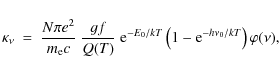
![\begin{displaymath}%
\tau_{\nu}(r)=\int^{r}_{r_{\rm max}} [\kappa_{\nu,\rm cont}...
...rm lines}(r')+\kappa_{\nu,\rm dust}(r')]~~ \rho(r')~ {\rm d}r'
\end{displaymath}](/articles/aa/full_html/2010/06/aa11899-09/img83.png)
![\begin{figure}
\par\includegraphics[width=8.8cm,clip]{11899fig05.ps}
\end{figure}](/articles/aa/full_html/2010/06/aa11899-09/img88.png)
![\begin{figure}
\par\includegraphics[width=8.7cm,clip]{11899fig06.ps}\vspace*{3mm}
\end{figure}](/articles/aa/full_html/2010/06/aa11899-09/img93.png)
![\begin{figure}
\par\includegraphics[width=8.8cm,clip]{11899fig07.ps}
\end{figure}](/articles/aa/full_html/2010/06/aa11899-09/img96.png)
![\begin{figure}
\par\includegraphics[width=8.8cm,clip]{11899fig08.ps}
\end{figure}](/articles/aa/full_html/2010/06/aa11899-09/img97.png)
![\begin{figure}
\par\includegraphics[width=8.4cm,clip]{11899fig09.ps}
\end{figure}](/articles/aa/full_html/2010/06/aa11899-09/img98.png)
![\begin{figure}
\par\includegraphics[width=8.4cm,clip]{11899fig10.ps}
\end{figure}](/articles/aa/full_html/2010/06/aa11899-09/img100.png)
![\begin{figure}
\par\includegraphics[width=8.4cm,clip]{11899fig11.ps}
\end{figure}](/articles/aa/full_html/2010/06/aa11899-09/img102.png)
![\begin{figure}
\par\includegraphics[width=8.5cm,clip]{11899fig12.ps}
\end{figure}](/articles/aa/full_html/2010/06/aa11899-09/img103.png)
![\begin{figure}
\par\includegraphics[width=8.5cm,clip]{11899fig13.ps}
\end{figure}](/articles/aa/full_html/2010/06/aa11899-09/img104.png)
![\begin{figure}
\par\includegraphics[width=8.5cm,clip]{11899fig14.ps}
\end{figure}](/articles/aa/full_html/2010/06/aa11899-09/img105.png)
![\begin{figure}
\par\includegraphics[width=8.5cm,clip]{11899fig15.ps}
\end{figure}](/articles/aa/full_html/2010/06/aa11899-09/img106.png)
![\begin{figure}
\par\includegraphics[width=8.5cm,clip]{11899fig16.ps}
\end{figure}](/articles/aa/full_html/2010/06/aa11899-09/img109.png)
![\begin{figure}
\par\includegraphics[width=16cm,clip]{11899fig17.ps}
\end{figure}](/articles/aa/full_html/2010/06/aa11899-09/img110.png)
![\begin{figure}
\par\includegraphics[width=8.3cm,clip]{11899fig18.ps}
\end{figure}](/articles/aa/full_html/2010/06/aa11899-09/img113.png)
![\begin{figure}
\par\includegraphics[width=8.5cm,clip]{11899fig19.ps}
\end{figure}](/articles/aa/full_html/2010/06/aa11899-09/img116.png)
![\begin{figure}
\par\includegraphics[width=8.5cm,clip]{11899fig20.ps}
\end{figure}](/articles/aa/full_html/2010/06/aa11899-09/img117.png)
![\begin{figure}
\par\includegraphics[width=8.5cm,clip]{11899fig21.ps}
\end{figure}](/articles/aa/full_html/2010/06/aa11899-09/img118.png)
![\begin{figure}
\par\includegraphics[width=17cm,clip]{11899fig22.ps}
\end{figure}](/articles/aa/full_html/2010/06/aa11899-09/img119.png)
![\begin{figure}
\par\includegraphics[width=8.8cm,clip]{11899figA1.ps} \vspace*{-1mm}
\end{figure}](/articles/aa/full_html/2010/06/aa11899-09/img124.png)
![\begin{figure}
\par\includegraphics[width=8.8cm,clip]{11899figA2.ps}
\end{figure}](/articles/aa/full_html/2010/06/aa11899-09/img125.png)
![\begin{figure}
\par\includegraphics[width=8.8cm,clip]{11899figA3.ps}
\end{figure}](/articles/aa/full_html/2010/06/aa11899-09/img126.png)
![\begin{figure}
\par\includegraphics[width=8.8cm,clip]{11899figA4.ps}
\end{figure}](/articles/aa/full_html/2010/06/aa11899-09/img127.png)
![\begin{figure}
\par\includegraphics[width=8.8cm,clip]{11899figA5.ps}
\end{figure}](/articles/aa/full_html/2010/06/aa11899-09/img128.png)
Current usage metrics show cumulative count of Article Views (full-text article views including HTML views, PDF and ePub downloads, according to the available data) and Abstracts Views on Vision4Press platform.
Data correspond to usage on the plateform after 2015. The current usage metrics is available 48-96 hours after online publication and is updated daily on week days.
Initial download of the metrics may take a while.