| Issue |
A&A
Volume 513, April 2010
|
|
|---|---|---|
| Article Number | A24 | |
| Number of page(s) | 6 | |
| Section | Astrophysical processes | |
| DOI | https://doi.org/10.1051/0004-6361/200913866 | |
| Published online | 16 April 2010 | |
The heliospheric transport and modulation of multiple charged anomalous oxygen revisited
R. D. Strauss - M. S. Potgieter - S. E. S. Ferreira
Unit for Space Physics, North-West University, 2520, Potchefstroom, South Africa
Received 14 December 2009 / Accepted 1 February 2010
Abstract
Context. Since the crossings of the solar wind termination
shock by the Voyager 1 and 2 spacecraft, much speculation has
surrounded the acceleration mechanism and region where the anomalous
cosmic ray component is accelerated. A peculiar, and mostly
overlooked feature of the observed anomalous oxygen spectrum near the
termination shock, is the power law form of the roll-over (cut-off) at
the high energy range of this spectrum.
Aims. We investigate, using a numerical model, why this
deviation from the expected exponential form of the cut-off part of the
anomalous oxygen spectrum occurs, and if the observed power law
form can be explained in terms of the acceleration of multiple charged
anomalous oxygen.
Methods. Multiple charged anomalous cosmic rays are incorporated
in a numerical model, based on the standard Parker transport equation,
including acceleration at the solar wind termination shock. This is
done by specifying an energy dependent charge state, constrained by
observations.
Results. Comparing computational results with spacecraft
observations, it is found that the inclusion of multiply charged
anomalous cosmic rays in the modulation model can explain the
observed spectrum of anomalous oxygen in the energy range from
10-70 MeV per nucleon. The more effective acceleration
of these multiple charge anomalous particles at the solar wind
termination shock causes a significant deviation from the usual
exponential cut-off spectrum to display instead a power law
decrease up to 70 MeV per nucleon where galactic oxygen
starts to dominate. In addition, the model reproduces the features
of multiple charged oxygen at Earth so that a good comparison is
obtained between computations and observations.
Key words: Sun: heliosphere - cosmic rays - acceleration of particles
1 Introduction
Anomalous cosmic ray (ACR) spectra are expected to decrease
exponentially above the energy where the acceleration of these
particles is getting ineffective. This feature of observed and modelled
ACR spectra is usually referred to as the roll-over or cut-off
spectrum, the latter indicative of the fact that the acceleration
process is progressively becoming less effective with further increases
in energy (e.g. Jokipii 1986; Potgieter & Moraal 1988). However, Webber et al. (2007),
who studied the temporal and spectral variations of
ACR oxygen (O*) nuclei at the Voyager 1 (V1)
and 2 (V2) spacecraft in the outer heliosphere from 1990 to
2006, reported that the observed O* spectra exhibited, for both V1
and V2, a clear power-law decrease with intensity
![]() at energies of 10 to 70 MeV nuc-1.
This is evidently in the roll-over range (see their Fig. 9).
To emphasize this feature of the observations, Fig. 1
shows the observed O* spectra from V1 during its TS crossing and
from V2 at about 4 AU from its TS crossing as reported by Webber
et al. (2007). For comparison a
at energies of 10 to 70 MeV nuc-1.
This is evidently in the roll-over range (see their Fig. 9).
To emphasize this feature of the observations, Fig. 1
shows the observed O* spectra from V1 during its TS crossing and
from V2 at about 4 AU from its TS crossing as reported by Webber
et al. (2007). For comparison a
![]() decrease is also shown in the figure, clearly illustrating that both
spectra decrease in this form. Note that above 50 MeV nuc-1,
the O* spectra contain a significant contribution from galactic
origin, which is not investigated further in this study as the level of
galactic oxygen at these energies is too low.
decrease is also shown in the figure, clearly illustrating that both
spectra decrease in this form. Note that above 50 MeV nuc-1,
the O* spectra contain a significant contribution from galactic
origin, which is not investigated further in this study as the level of
galactic oxygen at these energies is too low.
The spectra below 8 MeV nuc-1 are not shown in Fig. 1, neither investigated in this study because their peculiar behaviour remains a very controversial subject. This seemingly modulated portion of the ACR spectra has already been addressed previously by various authors, offering a wide range of explanations (and speculations). These include adiabatic heating (Langner et al. 2006; Ferreira et al. 2007), second order Fermi acceleration (e.g. Zhang 2006; Ferreira et al. 2007), transient events (e.g. Florinski & Zank 2006), preferred acceleration at the flanks (e.g. McComas & Schwadron 2006) and at the equatorial regions of the heliosphere (e.g. Langner & Potgieter 2006; Ngobeni & Potgieter 2008), energy cascade processes (e.g. Fisk & Gloeckler 2009) and magnetic reconnection occurring near the heliopause (e.g. Lazarian & Opher 2009). The applicability and validity of these processes have remained a topic of further investigation. See also the reviews by Potgieter (2008), Lee et al. (2009) and Florinski et al. (2009).
It is generally accepted that the seed population of ACRs is pick-up ions (PUIs) (Fisk et al. 1974),
formed by the ionization of interstellar neutrals, and then
getting accelerated to higher energies in the outer heliosphere (Pesses
et al. 1981). Because of the
singly ionized seed population it is thus expected that ACRs must also
be singly ionized. Earlier observations by Biswas et al. (1988), Adams et al. (1991) and Klecker et al. (1995) confirmed that low energy ACRs are indeed mostly singly ionized. Later measurements by Mewaldt et al. (1996b,a) indicated that ACR neon, nitrogen and oxygen contain a large fraction of higher charge states at energies E > 10 MeV nuc-1, and that the fraction of singly ACRs decreases as a function of kinetic energy, as shown in Fig. 2. For O*, the ![]() level for singly ionized nuclei (Q=1) occurs at
level for singly ionized nuclei (Q=1) occurs at ![]() MeV nuc-1, with the higher energy values being dominated by higher charge states.
MeV nuc-1, with the higher energy values being dominated by higher charge states.
![\begin{figure}
\par\includegraphics[width=7.5cm,clip]{13866f0.eps}
\end{figure}](/articles/aa/full_html/2010/05/aa13866-09/img9.png)
|
Figure 1:
Observed O* energy spectra from V1 during its TS crossing (filled
circles) and from V2 at 4 AU away from its TS crossing (open
circles). For comparison, a
|
| Open with DEXTER | |
These higher charge states can be explained in terms of electron
stripping occurring at the TS because of the finite acceleration time
of ACRs. Discussed by Jokipii (1996),
this is essentially a charge exchange process whereby ACRs lose
additional electrons by interacting with solar wind protons. The
possibility of charge exchange occurring in other regions of the
heliosphere (Chalov et al. 2007) are not investigated here. The importance of these higher charge states lies in the fact that the energy gain ![]() per TS crossing of ACRs is proportional to their charge Q=Ze,
per TS crossing of ACRs is proportional to their charge Q=Ze,
where
2 The modulation model
The omni-directional ACR distribution function
![]() is obtained numerically by solving the time dependent Parker transport equation (Parker 1965)
is obtained numerically by solving the time dependent Parker transport equation (Parker 1965)
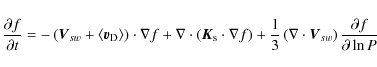
in terms of radial distance r, co-latitude (polar angle)
![\begin{figure}
\par\includegraphics[width=8cm,clip]{13866f1.eps}
\end{figure}](/articles/aa/full_html/2010/05/aa13866-09/img16.png)
|
Figure 2: The observed fraction of singly ionized ACR oxygen, neon and nitrogen as a function of kinetic energy. The data set is adapted from Mewaldt (2006). Because this fraction decreases with energy, ACRs are dominated by higher charge states (Q > 1) at higher energies, E > 10 MeV nuc-1. |
| Open with DEXTER | |
The PUIs, as source of ACRs, are introduced by specifying the source function as
| (3) |
It is assumed that
Useful in modulation studies, the specie value of the ACR population under consideration is defined as

where A is the atomic mass and Q is the charge of the particles. With A=16, singly ionized O* thus has a specie value of
where
![\begin{figure}
\par\includegraphics[width=8cm,clip]{13866f2.eps}
\end{figure}](/articles/aa/full_html/2010/05/aa13866-09/img41.png)
|
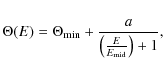
Figure 3:
The nett charge of the O* distribution function is scaled as a
function of kinetic energy using the transition given by Eq. (5). This figure shows the transitions for four different choices of
|
| Open with DEXTER | |
3 Modelling results and discussion
Computed energy O* spectra, with the inclusion of multiple charged ACRs, using the energy dependent transition of ![]() ,
are shown in Fig. 4 for the qA > 0 magnetic polarity cycle. Spectra are shown at the TS and at Earth, in the equatorial plane (
,
are shown in Fig. 4 for the qA > 0 magnetic polarity cycle. Spectra are shown at the TS and at Earth, in the equatorial plane (
![]() ). The four solutions shown correspond to the different specie
transitions discussed previously. The reference solutions (solid lines)
illustrate the general characteristics of these acceleration models,
which are briefly discussed next: below
). The four solutions shown correspond to the different specie
transitions discussed previously. The reference solutions (solid lines)
illustrate the general characteristics of these acceleration models,
which are briefly discussed next: below ![]() MeV nuc-1,
the TS spectra are dominated by the well known power law form
caused by Fermi I acceleration. This spectral index is
largely dependent on the TS compression ratio. With increasing
energy, intensities eventually start to fall away almost exponentially.
The energy at which this deviation in the power law spectrum
occurs is referred to as the cut-off or roll-over energy determined by,
amongst others, the curvature of the shock front (Steenberg &
Moraal 1999; Langner & Potgieter 2007). The spectra at Earth illustrate the corresponding modulated roll-over intensities; below
MeV nuc-1,
the TS spectra are dominated by the well known power law form
caused by Fermi I acceleration. This spectral index is
largely dependent on the TS compression ratio. With increasing
energy, intensities eventually start to fall away almost exponentially.
The energy at which this deviation in the power law spectrum
occurs is referred to as the cut-off or roll-over energy determined by,
amongst others, the curvature of the shock front (Steenberg &
Moraal 1999; Langner & Potgieter 2007). The spectra at Earth illustrate the corresponding modulated roll-over intensities; below ![]() MeV nuc-1 these spectra are dominated by adiabatic cooling giving rise to the well-known
MeV nuc-1 these spectra are dominated by adiabatic cooling giving rise to the well-known
![]() spectral shapes.
spectral shapes.
The effect of including additionally charged ACR can readily be seen in Fig. 4. The TS spectra (for all transition of ![]() )
show a large effect with the roll-over occurring at higher energies the
higher the charge state is made. Consequently, the O* intensities
in the roll-over energy range are higher for multiple charged ACR at a
given energy, leading to a factor
)
show a large effect with the roll-over occurring at higher energies the
higher the charge state is made. Consequently, the O* intensities
in the roll-over energy range are higher for multiple charged ACR at a
given energy, leading to a factor ![]() difference in intensities at
difference in intensities at ![]() MeV nuc-1 between the reference and
MeV nuc-1 between the reference and
![]() transitions (dottted line). Below the cut-off energy, the TS spectra remain completely unchanged.
transitions (dottted line). Below the cut-off energy, the TS spectra remain completely unchanged.
The spectra at Earth exhibit similar behaviour at higher energies, with
the intensities being higher in this energy regime for higher charge
states. In the adiabatic energy region the intensities are also
higher with the inclusion of higher charge states, with a factor ![]() difference between results from the different specie transitions.
difference between results from the different specie transitions.
Figure 5 is similar to Fig. 4 except that the results are shown for the qA < 0 magnetic
polarity cycle. The effect of incorporating multiple charged ACRs are
qualitatively similar to the results of the qA > 0 polarity
cycle, although the effect thereof in this cycle is much more
pronounced. Also evident is a clear intensity enhancement (flattening
of the power law part of the spectra) of the TS spectra at ![]() MeV nuc-1
just above the roll-over energy. This is believed to be caused by
drifts for this particular magnetic cycle. See also le Roux et al.
(1996), Jokipii & Kóta (1997) and Florinski & Jokipii (2003) for a discussion regarding this interesting phenomenon.
MeV nuc-1
just above the roll-over energy. This is believed to be caused by
drifts for this particular magnetic cycle. See also le Roux et al.
(1996), Jokipii & Kóta (1997) and Florinski & Jokipii (2003) for a discussion regarding this interesting phenomenon.
![\begin{figure}
\par\includegraphics[width=8cm,clip]{13866f3.eps}
\end{figure}](/articles/aa/full_html/2010/05/aa13866-09/img48.png)
|
Figure 4:
The computed O* energy spectra are shown at the TS (top set of curves) and at Earth (bottom set of curves) for the qA > 0 magnetic
polarity cycle. Four different spectra are shown, corresponding to the
computed solutions for the different transitions of
|
| Open with DEXTER | |
A comparison between computed and observed O* spectra at Earth is made in the left panel of Fig. 6. The observational data, measured by the SAMPEX spacecraft during the qA > 0 magnetic polarity cycle from 1993-1995, show both singly ionized (Q=1) and the total (Q=1+Q>1) O* spectra, adapted from Mewaldt (2006).
The data set does not represent solar minimum conditions, making
quantitative comparison with modelled solutions difficult so that
qualitative agreement will have to suffice. The deduction can be made
that the lower data points were observed in 1993. Evidently, from
Fig. 6, the singly ionized observations and reference model solution (i.e. without introducing higher charge states,
![]() )
show good agreement, while the total observed spectrum shows very good agreement with the
)
show good agreement, while the total observed spectrum shows very good agreement with the
![]() transition.
This agreement confirms that the method introduced here to incorporate
the effect of higher charge states in the modulation model is indeed
valid, and able to reproduce O* observations at Earth. We
interpret this good agreement as confirmation of the presence of higher
charge states in the observed O* population.
transition.
This agreement confirms that the method introduced here to incorporate
the effect of higher charge states in the modulation model is indeed
valid, and able to reproduce O* observations at Earth. We
interpret this good agreement as confirmation of the presence of higher
charge states in the observed O* population.
The right panel of Fig. 6 shows the modelled O* energy spectra at the TS for the different specie transitions considered throughout. In the range 10-70 MeV nuc-1, a clear
![]() decrease was observed (Webber et al. 2007),
as alluded to previously. The reference solution (dashed-dotted
line) is for a singly ionized ACR distribution only, resulting in
a spectrum falling off exponentially beyond the ACR roll-over energy.
The other computed solutions show how this exponential roll-over
gradually changes as multiple charge particles are introduced. While
the
decrease was observed (Webber et al. 2007),
as alluded to previously. The reference solution (dashed-dotted
line) is for a singly ionized ACR distribution only, resulting in
a spectrum falling off exponentially beyond the ACR roll-over energy.
The other computed solutions show how this exponential roll-over
gradually changes as multiple charge particles are introduced. While
the
![]() transition
is similar to the reference case at low energies, deviations from this
behaviour begin to occur so that the ACR roll-over spectrum is altered
into what appears to be a power-law decrease as the roll-over energy
shifts to much higher energies. This solution also shows the best
agreement with the observations in reproducing the observed
power law roll-over. All the higher charged ACR solutions
show a similar behaviour. Clearly, the exponential decay is modified to
an almost power law decrease in intensity for energies
transition
is similar to the reference case at low energies, deviations from this
behaviour begin to occur so that the ACR roll-over spectrum is altered
into what appears to be a power-law decrease as the roll-over energy
shifts to much higher energies. This solution also shows the best
agreement with the observations in reproducing the observed
power law roll-over. All the higher charged ACR solutions
show a similar behaviour. Clearly, the exponential decay is modified to
an almost power law decrease in intensity for energies
![]() MeV nuc-1.
MeV nuc-1.
As higher charge states were also observed for ACR neon and nitrogen (Mewaldt 2006), similar looking power law decreases are also expected for these populations at the TS and further investigation is warranted.
![\begin{figure}
\par\includegraphics[width=8cm,clip]{13866f4.eps}
\end{figure}](/articles/aa/full_html/2010/05/aa13866-09/img50.png)
|
Figure 5: Similar to Fig. 4, but for the qA < 0 magnetic polarity cycle. |
| Open with DEXTER | |
4 Conclusions
![\begin{figure}
\par\includegraphics[width=8cm,clip]{13866f5.eps}\hspace*{1.5cm}
\includegraphics[width=8cm,clip]{13866f6.eps}
\end{figure}](/articles/aa/full_html/2010/05/aa13866-09/img51.png)
|
Figure 6: The left panel shows the observed and computed O* spectra at Earth. The observations are adapted from Mewaldt (2006), and show both the singly ionized (Q=1) and total (Q=1+Q>1) energy spectra, with the latter including higher charge states. The different lines show model calculations for the different energy dependent charge states as discussed previously. The right panel shows similar results, but now at the TS. The V1 observations from Fig. 1 are also shown for comparison. |
| Open with DEXTER | |
We have included the effect of higher charge state in modelling O* intensities, by specifying an appropriate energy dependent charge state as constrained by the observations of Mewaldt et al. (1996a,b). We have showed that the low energy O* spectra (and therefore the intensities) remain relatively unchanged by the inclusion of these higher charge states because this energy region is dominated by the well known Fermi I (diffusive shock) acceleration power law at the TS, which is independent of the particle charge, or ionization state of the ACR population under consideration. The effect on the high energy portion of the O* spectra is more pronounced with the inclusion of the multiple charged ACRs. The ACR roll-over energy moves to higher energies for the higher charge states at the TS, creating an increase in high energy O* intensities throughout the heliosphere. This increase in O* intensities is also reflected in the modulated spectra at Earth, with the low energy portion of these spectra again remaining relatively unaltered.
Introducing an energy dependent charge state, as outlined in this article, we are able to reproduce both the singly ionized (Q=1), as well as the total (with the inclusion of higher charge states, Q=1+Q>1) observed O* spectra at Earth, confirming that O* does consist of a large fraction of higher charge states at high energies, and more importantly, confirming that the effect of multiple charge O* must be included into a modulation model to correctly reproduce the observed high energy O* spectra.
Using the same approach in the outer heliosphere, we are able to reproduce the observed
![]() decrease in intensity (Webber et al. 2007) observed by the V1 spacecraft at the TS for O* in the energy range 10-70 MeV nuc-1.
This deviation from the expected exponential form can thus be
attributed to multiple charged ACRs being both present and even
dominant at high energies. Furthermore it is concluded that this almost
power law behaviour is not characteristic of any additional
acceleration mechanisms but due to the more efficient acceleration of
higher charge states.
decrease in intensity (Webber et al. 2007) observed by the V1 spacecraft at the TS for O* in the energy range 10-70 MeV nuc-1.
This deviation from the expected exponential form can thus be
attributed to multiple charged ACRs being both present and even
dominant at high energies. Furthermore it is concluded that this almost
power law behaviour is not characteristic of any additional
acceleration mechanisms but due to the more efficient acceleration of
higher charge states.
The fact that this model can reproduce the power-law form of the observed high energy portion (E > 20 MeV nuc-1)
of the O* spectra so well can be interpreted that diffusive shock
acceleration of multiple charged O* is indeed occurring near and
at the TS, and that this process is primarily responsible for
accelerating O* to such high energies. However, it appears
that diffusive shock acceleration, as the only acceleration
mechanism, cannot account for the modulated form of the low energy
ACR spectra (
![]() MeV nuc-1)
at the TS and their subsequent unfolding into the heliosheath. This
indicates that the process is indeed very complex, with additional
re-acceleration of ACRs in the heliosheath required or that it may be
attributed to specific heliospheric geometries, causing more effective
acceleration elsewhere at the TS, or that the seed particle
distribution for ACRs is less straightforward than previously assumed,
as the latest IBEX results may suggest. Clearly, more observations
and modelling efforts are needed to constrain these physical processes
further, and until then, it will remain a controversial topic.
MeV nuc-1)
at the TS and their subsequent unfolding into the heliosheath. This
indicates that the process is indeed very complex, with additional
re-acceleration of ACRs in the heliosheath required or that it may be
attributed to specific heliospheric geometries, causing more effective
acceleration elsewhere at the TS, or that the seed particle
distribution for ACRs is less straightforward than previously assumed,
as the latest IBEX results may suggest. Clearly, more observations
and modelling efforts are needed to constrain these physical processes
further, and until then, it will remain a controversial topic.
The authors wish to thank W.R. Webber and M.E. Hill for informative research discussions.
References
- Adams, J. H., Gracia-Munoz, M., Grigorov, N. L., et al. 1991, Proc. Int. Cosmic Ray Conf., 3, 358 [Google Scholar]
- Biswas, S., Durgaprasad, N., Mitra, B., et al. 1988, Astrophys. Space Sci., 149, 357 [NASA ADS] [CrossRef] [Google Scholar]
- Burger, R. A., Potgieter, M. S., & Heber, B. 2000, J. Geophys. Res., 105, 27447 [Google Scholar]
- Chalov, S. V., Fahr, H. J., & Malama, Y. G. 2007, Ann. Geophys., 25, 575 [Google Scholar]
- Ferreira, S. E. S., Potgieter, M. S., & Scherer, K. 2007, J. Geophys. Res., 112, 11101 [Google Scholar]
- Fisk, L. A., & Gloeckler, G. 2009, Adv. Space Res., 43, 1471 [NASA ADS] [CrossRef] [Google Scholar]
- Fisk, L. A., Kozlovsky, B., & Ramaty, R. 1974, ApJ, 190, L35 [NASA ADS] [CrossRef] [Google Scholar]
- Florinski, V., & Jokipii, J. R. 2003, ApJ, 591, 454 [NASA ADS] [CrossRef] [Google Scholar]
- Florinksi, V., & Zank, G. P. 2006, Geophys. Res. Lett., 33, 15110 [NASA ADS] [CrossRef] [Google Scholar]
- Florinksi, V., Balogh, A., Jokipii, J. R., et al. 2009, Space Sci. Rev., 143, 57 [NASA ADS] [CrossRef] [Google Scholar]
- Jokipii, J. R. 1986, J. Geophys. Res., 91, 2929 [NASA ADS] [CrossRef] [Google Scholar]
- Jokipii, J. R. 1990, in Physics of the Outer Heliosphere, ed. S. Grzedzielski, & D. E. Page (Oxford: Pergamon Press), 169 [Google Scholar]
- Jokipii, J. R. 1996, ApJ, 466, L47 [NASA ADS] [CrossRef] [Google Scholar]
- Jokipii, J. R., & Kóta, J. 1989, J. Geophys. Res., 16, 1 [Google Scholar]
- Jokipii, J. R., & Kóta. 1997, Proc. Int. Cosmic Ray Conf., 8, 151 [Google Scholar]
- Klecker, B., McNab, M. C., Blake, J. B., et al. 1995, ApJ, 442, L69 [NASA ADS] [CrossRef] [Google Scholar]
- Langner, U. W., & Potgieter, M. S. 2006, in Acceleration of galactic and anomalous cosmic rays in the heliosheath, ed. J. Heerikhuisen, V. Florinski, G. P. Zank, et al. (New York: AIP), 858, 233 [Google Scholar]
- Langner, U. W., & Potgieter, M. S. 2007, Adv. Space Res., 41, 368 [NASA ADS] [CrossRef] [Google Scholar]
- Langner, U. W., Potgieter, M. S., & Webber, W. R. 2003, J. Geophys. Res., 108, 8039 [CrossRef] [Google Scholar]
- Langner, U. W., Potgieter, M. S., & Webber, W. R. 2004, Adv. Space Res., 34, 138 [NASA ADS] [CrossRef] [Google Scholar]
- Langner, U. W., Potgieter, M. S., Fichtner, H., et al. 2006, J. Geophys. Res., 111, A101106 [Google Scholar]
- Lazarian, A., & Opher, M. 2009, ApJ, 703, 8 [NASA ADS] [CrossRef] [Google Scholar]
- Lee, M. A., Fahr, H. J., & Kucharek, H. 2009, Space Sci. Rev., 146, 275 [NASA ADS] [CrossRef] [Google Scholar]
- le Roux, J. A., Potgieter, M. S., & Ptuskin, V. S. 1996, J. Geophys. Res., 101, 4791 [NASA ADS] [CrossRef] [Google Scholar]
- McComas, D. J., & Schwadron, N. A. 2006, Geophys. Res. Lett., 33, 4102 [NASA ADS] [CrossRef] [Google Scholar]
- Mewaldt, R. A. 2006, in Physics of the Inner Heliosheath, ed. J. Heerikhuisen, V. Florinski, G. P. Zank, et al. (New York: AIP), 858, 92 [Google Scholar]
- Mewaldt, R. A., Cummings, J. R., Leske, R. A., et al. 1996a, Geophys. Res. Lett., 23, 617 [NASA ADS] [CrossRef] [Google Scholar]
- Mewaldt, R. A., Selesnick, R. S., Cummings, J. R., et al. 1996b, ApJ, 466, L43 [NASA ADS] [CrossRef] [Google Scholar]
- Minnie, J., Bieber, J. W., Matthaeus, W. H., et al. 2007, ApJ, 670, 1149 [NASA ADS] [CrossRef] [Google Scholar]
- Ngobeni, M. D., & Potgieter, M. S. 2008, Adv. Space Res., 41, 373 [Google Scholar]
- Parker, E. N. 1958, ApJ, 128, 664 [Google Scholar]
- Parker, E. N. 1965, Planet. Space. Sci., 13, 9 [NASA ADS] [CrossRef] [Google Scholar]
- Pesses, M. E., Eichler, D., & Jokippi, J. R. 1981, ApJ, 246, L85 [NASA ADS] [CrossRef] [Google Scholar]
- Potgieter, M. S. 1989, Adv. Space. Res., 9, 1989 [Google Scholar]
- Potgieter, M. S. 2008, Adv. Space. Res., 41, 245 [Google Scholar]
- Potgieter, M. S., & Moraal, H. 1988, ApJ, 330, 445 [NASA ADS] [CrossRef] [Google Scholar]
- Richardson, J. D., Kasper, J. C., Wang, C., et al. 2008, Nature, 454, 63 [NASA ADS] [CrossRef] [PubMed] [Google Scholar]
- Steenberg, C. D., & Moraal, H. 1999, J. Geophys. Res., 104, 24879 [Google Scholar]
- Webber, W. R., Cummings, A. C., McDonald, F. B., et al. 2007, J. Geophys. Res., 112, 6105 [Google Scholar]
- Zank, G. P., Matthaeus, W. H., & Smith, C. W. 1996, J. Geophys. Res., 101, 17093 [NASA ADS] [CrossRef] [Google Scholar]
- Zhang, M. 2006, in Acceleration of galactic and anomalous cosmic rays in the heliosheath, ed. J. Heerikhuisen, V. Florinski, G. P. Zank, et al. (New York: AIP), 858, 226 [Google Scholar]
All Figures
|
|
Figure 1:
Observed O* energy spectra from V1 during its TS crossing (filled
circles) and from V2 at 4 AU away from its TS crossing (open
circles). For comparison, a
|
| Open with DEXTER | |
| In the text | |
|
|
Figure 2: The observed fraction of singly ionized ACR oxygen, neon and nitrogen as a function of kinetic energy. The data set is adapted from Mewaldt (2006). Because this fraction decreases with energy, ACRs are dominated by higher charge states (Q > 1) at higher energies, E > 10 MeV nuc-1. |
| Open with DEXTER | |
| In the text | |
|
|
Figure 3:
The nett charge of the O* distribution function is scaled as a
function of kinetic energy using the transition given by Eq. (5). This figure shows the transitions for four different choices of
|
| Open with DEXTER | |
| In the text | |
|
|
Figure 4:
The computed O* energy spectra are shown at the TS (top set of curves) and at Earth (bottom set of curves) for the qA > 0 magnetic
polarity cycle. Four different spectra are shown, corresponding to the
computed solutions for the different transitions of
|
| Open with DEXTER | |
| In the text | |
|
|
Figure 5: Similar to Fig. 4, but for the qA < 0 magnetic polarity cycle. |
| Open with DEXTER | |
| In the text | |
|
|
Figure 6: The left panel shows the observed and computed O* spectra at Earth. The observations are adapted from Mewaldt (2006), and show both the singly ionized (Q=1) and total (Q=1+Q>1) energy spectra, with the latter including higher charge states. The different lines show model calculations for the different energy dependent charge states as discussed previously. The right panel shows similar results, but now at the TS. The V1 observations from Fig. 1 are also shown for comparison. |
| Open with DEXTER | |
| In the text | |
Copyright ESO 2010
Current usage metrics show cumulative count of Article Views (full-text article views including HTML views, PDF and ePub downloads, according to the available data) and Abstracts Views on Vision4Press platform.
Data correspond to usage on the plateform after 2015. The current usage metrics is available 48-96 hours after online publication and is updated daily on week days.
Initial download of the metrics may take a while.