| Issue |
A&A
Volume 513, April 2010
|
|
|---|---|---|
| Article Number | A17 | |
| Number of page(s) | 10 | |
| Section | Astrophysical processes | |
| DOI | https://doi.org/10.1051/0004-6361/200913495 | |
| Published online | 15 April 2010 | |
Escape-limited model of cosmic-ray acceleration revisited
Y. Ohira1 - K. Murase2 - R. Yamazaki3
1 - Department of Earth and Space Science, Osaka University, Toyonaka 560-0043, Japan
2 -
Yukawa Institute for Theoretical Physics, Kyoto University, Kyoto 606-8502, Japan
3 -
Department of Physical Science, Hiroshima University, Higashi-Hiroshima 739-8526, Japan
Received 19 October 2009 / Accepted 10 January 2010
Abstract
Context. The spectrum of cosmic rays (CRs) is affected by
their escape from an acceleration site. This may be observed not only
in the gamma-ray spectrum of young supernova remnants (SNRs) such as
RX J1713.7-3946, but also in the spectrum of CRs showering the
Earth.
Aims. The escape-limited model of cosmic-ray acceleration is
studied in general. We discuss the spectrum of runaway CRs from the
acceleration site. The model will also be able to constrain the
spectral index at the acceleration site and the ansatz with respect to
the unknown injection process into the particle acceleration.
Methods. Our methods are analytical derivations. We apply our
model to CR acceleration in SNRs and in active galactic nuclei
(AGN), which are plausible candidates of Galactic and
extragalactic CRs, respectively. In particular we take
account into the shock evolution with cooling of escaping CRs in the
Sedov phase for young SNRs.
Results. The spectrum of escaping CRs generally depends on the
physical quantities at the acceleration site like the spectral index,
the evolution of the maximum energy of CRs and the evolution of the
normalization factor of the spectrum. It is found that the
spectrum of runaway particles can be both softer and harder than that
of the acceleration site.
Conclusions. The model explains spectral indices of both
Galactic and extragalactic CRs produced by SNRs and AGNs, respectively,
suggesting the unified picture of CR acceleration.
Key words: acceleration of particles - cosmic rays - ISM: supernova remnants - galaxies: jets
1 Introduction
The origin of cosmic rays (CRs) has been one of the long-standing
problems. The number spectrum of nuclear CRs observed at the
Earth,
![]() ,
shows a break at the ``knee'' energy (
,
shows a break at the ``knee'' energy (
![]() eV), below which the spectral index is about
eV), below which the spectral index is about
![]() (Cronin 1999).
Because of the energy-dependent propagation of CRs, the spectral shape
at the source is different from that observed on Earth. Taking into
account the propagation effect, the source spectral index has been well
constrained as
(Cronin 1999).
Because of the energy-dependent propagation of CRs, the spectral shape
at the source is different from that observed on Earth. Taking into
account the propagation effect, the source spectral index has been well
constrained as
![]() in various models (e.g., Strong & Moskalenko 1998; Putze et al. 2009). This value of s has been also inferred to explain the Galactic diffuse gamma-ray emission (e.g., Strong et al. 2000). This may give us valuable insights into the acceleration mechanism of CRs.
in various models (e.g., Strong & Moskalenko 1998; Putze et al. 2009). This value of s has been also inferred to explain the Galactic diffuse gamma-ray emission (e.g., Strong et al. 2000). This may give us valuable insights into the acceleration mechanism of CRs.
Mechanisms of CR acceleration have also been studied for a long time,
and the most plausible process is a diffusive shock acceleration (DSA) (Blandford & Ostriker 1978; Krymsky 1977; Axford et al. 1977; Bell 1978).
Very high-energy gamma-ray observations have revealed the existence of
high-energy particles at the shock of young supernova remnants (SNRs),
which supports the DSA mechanism as well as the paradigm that the
Galactic CRs are produced by young SNRs (e.g., Enomoto et al. 2002; Katagiri et al. 2005; Aharonian et al. 2005,2004).
Recent progress of the theory of DSA revealed that the back-reactions
of accelerated CRs are important if a large number of nuclear particles
are accelerated (Malkov & Drury 2001; Drury & Völk 1981).
There are several observational facts which are consistent with the predictions of such a nonlinear model (Bamba et al. 2005b; Warren et al. 2005; Bamba et al. 2005a; Uchiyama et al. 2007; Bamba et al. 2003; Helder et al. 2009; Vink & Laming 2003). The model predicts, however, the harder spectrum of accelerated particles at the shock than
![]() (corresponding to s=2) where p is the momentum of CRs, in particular, near the knee energy (Malkov 1997; Kang et al. 2001; Berezhko & Ellison 1999). This apparently contradicts the source spectral index of
(corresponding to s=2) where p is the momentum of CRs, in particular, near the knee energy (Malkov 1997; Kang et al. 2001; Berezhko & Ellison 1999). This apparently contradicts the source spectral index of
![]() inferred from the CR spectrum on Earth. Even in the test-particle
limit of DSA, such a soft source spectrum requires a shock with the
small Mach number (
inferred from the CR spectrum on Earth. Even in the test-particle
limit of DSA, such a soft source spectrum requires a shock with the
small Mach number (![]() ), which is unexpected for young SNRs.
), which is unexpected for young SNRs.
There are several models of DSA, depending on the boundary conditions
imposed. Different models predict different spectra of CRs dispersed
from the shock region. So far, the age-limited acceleration has
been frequently considered as a representative case (Sect. 2).
In this model, all the particles are stored around the shock while
accelerated. When the confinement becomes inefficient, all the
particles run away from the region at a time. Then the source spectrum
of CRs which has just escaped from the acceleration region is expected
to be the same as that at the shock front. Therefore, this model
predicts that the source spectrum is the same as that of accelerated
particles, which is typically harder than the observed one.
In this paper, we consider an alternative model, the
escape-limited acceleration, to explain the observed
CR spectrum on Earth
(Sect. 3). This model is
preferable to the age-limited acceleration when we consider
observational results for young SNR RX J1713.7-3946, of which
TeV ![]() -ray emission is more precisely measured than any others (Sect. 4.1).
-ray emission is more precisely measured than any others (Sect. 4.1).
The nature of CRs with energies much higher than the knee energy is also still uncertain.
While CRs below the second knee (
![]() eV) may be of Galactic origin, the highest energy CRs above
eV) may be of Galactic origin, the highest energy CRs above
![]() eV are believed to be extragalactic. Possible candidates are active galactic nuclei (AGNs) (e.g., Rachen & Biermann 1993; Takahara 1990; Pe'er et al. 2009; Biermann & Strittmatter 1987), gamma-ray bursts (Murase et al. 2006; Waxman 1995; Vietri 1995), magnetars (Arons 2003; Murase et al. 2009) and clusters of galaxies (Inoue et al. 2007; Kang et al. 1997). The intermediate energy range from
eV are believed to be extragalactic. Possible candidates are active galactic nuclei (AGNs) (e.g., Rachen & Biermann 1993; Takahara 1990; Pe'er et al. 2009; Biermann & Strittmatter 1987), gamma-ray bursts (Murase et al. 2006; Waxman 1995; Vietri 1995), magnetars (Arons 2003; Murase et al. 2009) and clusters of galaxies (Inoue et al. 2007; Kang et al. 1997). The intermediate energy range from
![]() eV to
eV to
![]() eV
is more uncertain. Both the Galactic and extragalactic origins are
possible and it may just be a transition between the two.
As the extragalactic origin, AGNs (Berezinsky et al. 2006), clusters of galaxies (Murase et al. 2008) and hypernovae (Wang et al. 2007) have been proposed so far.
eV
is more uncertain. Both the Galactic and extragalactic origins are
possible and it may just be a transition between the two.
As the extragalactic origin, AGNs (Berezinsky et al. 2006), clusters of galaxies (Murase et al. 2008) and hypernovae (Wang et al. 2007) have been proposed so far.
Among these possibilities, AGN are one of the most plausible candidates
for accelerators of high-energy CRs, because they can explain the ultra
high energy cosmic-ray (UHECR) spectrum above
![]() eV assuming the proton composition. In such a proton dip model, the source spectrum of UHECRs is
eV assuming the proton composition. In such a proton dip model, the source spectrum of UHECRs is
![]() with
s=2.4-2.7, depending on the models of the source evolution (Berezinsky et al. 2006). The required source spectral index of
s=2.4-2.7 can be explained by several possibilities. First,
it can be attributed to the acceleration mechanism itself. One can
consider non-Fermi acceleration mechanisms (Berezinsky et al. 2006) or the two-step diffusive shock acceleration in two different shocks (Aloisio et al. 2007).
Second, the index can be attributed to a superposition of many
AGNs with different maximum energies, and one can suppose that AGNs
with different luminosities may have different maximum energies (Kachelriess & Semikoz 2006). Recently, Berezhko (2008)
proposed another possibility with the cocoon shock model. In this
cocoon shock scenario, different maximum energies can be interpreted as
maximum energies of escaping particles at different ages of
AGN jets. Although it is very uncertain whether efficient
CR acceleration occurs
there, this scenario would also be one of the possibilities to be
investigated in detail.
with
s=2.4-2.7, depending on the models of the source evolution (Berezinsky et al. 2006). The required source spectral index of
s=2.4-2.7 can be explained by several possibilities. First,
it can be attributed to the acceleration mechanism itself. One can
consider non-Fermi acceleration mechanisms (Berezinsky et al. 2006) or the two-step diffusive shock acceleration in two different shocks (Aloisio et al. 2007).
Second, the index can be attributed to a superposition of many
AGNs with different maximum energies, and one can suppose that AGNs
with different luminosities may have different maximum energies (Kachelriess & Semikoz 2006). Recently, Berezhko (2008)
proposed another possibility with the cocoon shock model. In this
cocoon shock scenario, different maximum energies can be interpreted as
maximum energies of escaping particles at different ages of
AGN jets. Although it is very uncertain whether efficient
CR acceleration occurs
there, this scenario would also be one of the possibilities to be
investigated in detail.
The organization of the paper is as follows. After the brief introduction of the age-limited model of the CR acceleration (Sect. 2), we study the escape-limited model in Sect. 3. For a simple understanding, the general argument in a stationary, test-particle approximation is given in Sect. 3.1. Then we derive the formulae of the maximum energy of accelerated particles in Sect. 3.2 and of the spectrum of escaping particles in Sect. 3.3. We consider the applications to young SNR and AGN in Sects. 4 and 5, respectively. Section 6 is devoted to a discussion.
2 Maximum attainable momentum in the age-limited acceleration
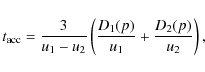
For comparison with the escape-limited acceleration, we briefly
summarize the case of the age-limited acceleration. In this case,
the maximum momentum of accelerated particles
![]() is determined by
is determined by
![]() ,
where
,
where
![]() and
and
![]() are the age of the shock and the acceleration time scale, respectively.
When we consider DSA,
are the age of the shock and the acceleration time scale, respectively.
When we consider DSA,
![]() is given by (Drury 1983)
is given by (Drury 1983)
|
(1) |
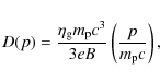
where D(p) and u are the diffusion coefficient as a function of the momentum of accelerated particles and the velocity of the background fluid, respectively. Subscripts 1 and 2 represent upstream and downstream regions, respectively. For simplicity, we assume the Bohm-type diffusion, i.e.,
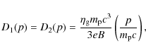
where B,
3 Escape-limited acceleration
In the framework of DSA, accelerated particles are scattered by the turbulent magnetic field and go back and forth across the shock front. Upstream turbulence may be excited by the accelerated particles themselves (Bell 1978), and the magnetic field strength of this turbulence is theoretically expected to be strong (e.g., Lucek & Bell 2000). There are observational evidences suggesting that CRs are responsible for substantial amplification of the ambient magnetic field in the precursors of shock fronts in SNRs and that such magnetic turbulence well confines the particles around the shock front (Yamazaki et al. 2004; Bamba et al. 2005b,a; Uchiyama et al. 2007; Bamba et al. 2003; Vink & Laming 2003; Parizot et al. 2006), leading to the efficient CR acceleration.
The spectrum of accelerated particles is affected by the spatial and
spectral structures of the magnetic turbulence through the process in
which the particles escape from the shock toward far upstream regions.
There are mainly two scenarios of the escape model considered
so far; one causes the effect on the boundary in the momentum
space, and the other causes the effect on the spatial boundary. The
former comes from significant decay of the wave amplitude below the
wave number ![]() of the turbulence spectrum (Drury et al. 2009; Reynolds 1998). Particles with the Lorentz factor above
of the turbulence spectrum (Drury et al. 2009; Reynolds 1998). Particles with the Lorentz factor above
![]() satisfying the resonance condition,
satisfying the resonance condition,
![]() ,
where
,
where
![]() is the cyclotron frequency, are not confined around the shock front and
escape into far upstream regions. In this context, the escape flux
was calculated previously (e.g., Ptuskin & Zirakashvili 2005; Drury et al. 2009). The latter effect has been recently discussed by several authors (Ptuskin & Zirakashvili 2005; Reville et al. 2009; Caprioli et al. 2009).
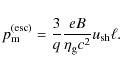
The turbulence generation may be connected with the flux of accelerated
particles themselves. Hence, in the region far from the shock
front, the flux of high-energy particles is small and wave excitation
is less significant. If the accelerated particles reach the
region, they are dispersed into the far upstream region. Let
is the cyclotron frequency, are not confined around the shock front and
escape into far upstream regions. In this context, the escape flux
was calculated previously (e.g., Ptuskin & Zirakashvili 2005; Drury et al. 2009). The latter effect has been recently discussed by several authors (Ptuskin & Zirakashvili 2005; Reville et al. 2009; Caprioli et al. 2009).
The turbulence generation may be connected with the flux of accelerated
particles themselves. Hence, in the region far from the shock
front, the flux of high-energy particles is small and wave excitation
is less significant. If the accelerated particles reach the
region, they are dispersed into the far upstream region. Let ![]() be the distance from the shock beyond which the amplitude of the
upstream turbulence becomes negligible. Characteristic spatial length
of particles penetrating into the upstream region is given by
be the distance from the shock beyond which the amplitude of the
upstream turbulence becomes negligible. Characteristic spatial length
of particles penetrating into the upstream region is given by
![]() .
As long as
.
As long as
![]() ,
the particles are confined without the significant escape loss,
and they are accelerated to higher energies. On the other hand, when
their momentum increases up to sufficiently high energies satisfying
,
the particles are confined without the significant escape loss,
and they are accelerated to higher energies. On the other hand, when
their momentum increases up to sufficiently high energies satisfying
![]() ,
their acceleration ceases and they escape into the far upstream.
Therefore, the maximum momentum of accelerated particles in this
scenario is given by the condition
,
their acceleration ceases and they escape into the far upstream.
Therefore, the maximum momentum of accelerated particles in this
scenario is given by the condition
![]() .
Below we consider the escape-limited model, where the maximum energy is essentially determined by
.
Below we consider the escape-limited model, where the maximum energy is essentially determined by
![]() .
.
3.1 A simple case of stationary, test-particle approximation
In order to take an essential feature of the escape-limited
acceleration, we calculated the escape flux and the maximum attainable
energy of accelerated particles for the simplest case (see also Caprioli et al. 2009). Let us consider the stationary transport equation
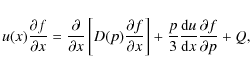
with the boundary condition
where u1 and u2 are constants. The solution to the transport equation in the test-particle approximation is derived as (Caprioli et al. 2009)
![\begin{displaymath}%
f(x,p)=f_0(p)
\frac{\exp\left[\frac{u_1x}{D(p)}\right]-\exp...
...ell}{D(p)}\right]}
{1-\exp\left[-\frac{u_1\ell}{D(p)}\right]},
\end{displaymath}](/articles/aa/full_html/2010/05/aa13495-09/img41.png)
|
(6) |
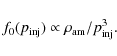
where f0(p)=f(x=0,p) is given by
![\begin{displaymath}%
f_0(p)=K\exp\left\{
-q\int_{p_{\rm inj}}^p\frac{{\rm d}\log p'}
{1-\exp\left[-\frac{u_1\ell}{D(p')}\right]}
\right\},
\end{displaymath}](/articles/aa/full_html/2010/05/aa13495-09/img42.png)
and q=3u1/(u1-u2). The escape flux at
| |
= | 
|
|
| = | ![$\displaystyle \frac{u_1f_0(p)}{1-\exp\left[\frac{u_1\ell}{D(p)}\right]}\cdot$](/articles/aa/full_html/2010/05/aa13495-09/img45.png)
|
(8) |
Let us introduce a new variable
![\begin{displaymath}%
\frac{{\rm d}\Phi}{{\rm d} y} = -\frac{1}{1-\exp\left[-\fra...
...t[q-\frac{u_1\ell}{D(y)}\frac{{\rm d}\ln D}{{\rm d} y}\right],
\end{displaymath}](/articles/aa/full_html/2010/05/aa13495-09/img50.png)
|
(9) |
| |
= | ![$\displaystyle \frac{\frac{u_1\ell}{D(y)}}
{\left\{1-\exp\left[-\frac{u_1\ell}{D...
...)}\frac{{\rm d}\ln D}{{\rm d} y} \right]
\frac{{\rm d}\ln D}{{\rm d} y} \right.$](/articles/aa/full_html/2010/05/aa13495-09/img52.png)
|
|
![$\displaystyle \left. + ~
\left[1-\exp\left[-\frac{u_1\ell}{D(y)}\right]\right]
...
...}\ln D}{{\rm d} y}\right)^2-
\frac{\partial^2\ln D}{\partial y^2} \right\}\cdot$](/articles/aa/full_html/2010/05/aa13495-09/img53.png)
|
(10) |
Below we consider the case of Bohm diffusion,
(where
| |
= | 
|
|
| = | ![$\displaystyle \ln\left[
\frac{u_1f_0(p_{\rm m})}{1-e^{-q}}\right]
-\left(\frac{y-y_{\rm m}}{\xi}\right)^2 + \cdots,$](/articles/aa/full_html/2010/05/aa13495-09/img59.png)
|
(12) |
where
Finally, going back to the function ![]() ,
we obtain
,
we obtain
![\begin{displaymath}%
\phi(p) = \frac{u_1f_0(p_{\rm m})}{1-e^{-q}}
\exp\left[-\left(\frac{\ln p-\ln p_{\rm m}}{\xi}\right)^2
+\cdots\right].
\end{displaymath}](/articles/aa/full_html/2010/05/aa13495-09/img67.png)
One can clearly see from Eq. (13) that particles with momentum around
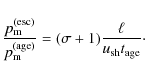
3.2 The maximum energy of accelerated particles
We have seen in Sect. 3.1 that in the stationary, test-particle case the quantity ![]() given by Eq. (11)
plays the role of maximum momentum of the accelerated particles at
the shock. Taking this into account, we assume that in the more
general escape-limited case the maximum momentum
given by Eq. (11)
plays the role of maximum momentum of the accelerated particles at
the shock. Taking this into account, we assume that in the more
general escape-limited case the maximum momentum
![]() is determined by
is determined by

Given that
|
(15) |
which is the same as in the age-limited case (Eq. (2) in Sect. 2), we obtain
Since
Hence, as long as
3.3 The spectrum of CRs dispersed from an accelerator
In this subsection, we derive the time-integrated spectrum of CR particles which is dispersed from an accelerator. The derivation is essentially identical to that of Ptuskin & Zirakashvili (2005). However, our argument is simpler and more general, so the final form of the spectrum (Eqs. (27) and (28)) is more general. Note that our formalism is applicable not only to DSA but also to arbitrary acceleration processes.
The proton production rate
![]() ,
at a certain epoch labeled by a parameter
,
at a certain epoch labeled by a parameter ![]() ,
is defined as the number of protons with momentum between p and
,
is defined as the number of protons with momentum between p and
![]() ,
which is produced in the interval between
,
which is produced in the interval between ![]() and
and
![]() .
Here
.
Here ![]() is the parameter which describes the dynamical evolution of the
accelerator - it can be either simply the age or the position of
the shock front. It is expected that
is the parameter which describes the dynamical evolution of the
accelerator - it can be either simply the age or the position of
the shock front. It is expected that ![]() contains the term of exponential cutoff at the momentum
contains the term of exponential cutoff at the momentum
![]() which depends on
which depends on ![]() (see, for example, Eq. (25)). The number of protons with momentum between p and
(see, for example, Eq. (25)). The number of protons with momentum between p and
![]() which is escaping from the accelerator at the epoch between
which is escaping from the accelerator at the epoch between ![]() and
and
![]() ,
is denoted by
,
is denoted by
![]() ,
and we assume
,
and we assume
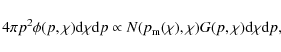
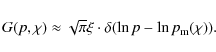
where
![\begin{displaymath}%
G(p,\chi)=
\exp\left[-\left(\frac{\ln p-\ln p_{\rm m}(\chi)}{\xi}\right)^2\right],
\end{displaymath}](/articles/aa/full_html/2010/05/aa13495-09/img85.png)
and
The time-integrated spectrum of protons which have escaped at the source
![]() is obtained by
is obtained by
In order to derive a simple analytical form, we approximate Eq. (19) as
If we use a general mathematical formula for
![\begin{displaymath}%
\delta(g(\chi)) =
\frac{\delta(\chi-\chi_0)}
{\left[\frac{{\rm d} g}{{\rm d}\chi}\right]_{\chi=\chi_0}},
\end{displaymath}](/articles/aa/full_html/2010/05/aa13495-09/img92.png)
|
(22) |
where
![\begin{displaymath}%
G(p,\chi)\propto
\frac{p_{\rm m}(\chi)}
{\left[\frac{{\rm ...
...ight]_{\chi=p_{\rm m}^{-1}(p)}}\delta(\chi-p_{\rm m}^{-1}(p)),
\end{displaymath}](/articles/aa/full_html/2010/05/aa13495-09/img94.png)
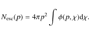
where
![\begin{displaymath}%
N_{\rm esc}(p) \propto
\frac{p N(p,p_{\rm m}^{-1}(p))}{p_{\...
... p_{\rm m}}{{\rm d}\chi}\right]_{\chi=p_{\rm m}^{-1}(p)}}\cdot
\end{displaymath}](/articles/aa/full_html/2010/05/aa13495-09/img98.png)
This is the most general analytical formula of the spectrum of protons dispersed from an accelerator.
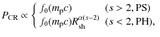
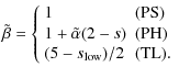
For the remainder of the paper, the form of ![]() is assumed to have
is assumed to have

![$\displaystyle \times ~ \exp\left[-\left(\frac{p}{p_{\rm m}(\chi)}\right)\right]
{\rm d}\log\chi~{\rm d} p,$](/articles/aa/full_html/2010/05/aa13495-09/img101.png)
which is a power law with the index s and the exponential cut off at
![\begin{displaymath}%
N_{\rm esc}(p)\propto
\frac{p^{1-s}K\left(p_{\rm m}^{-1}(p)...
... p_{\rm m}}{{\rm d}\chi}\right]_{\chi=p_{\rm m}^{-1}(p)}}\cdot
\end{displaymath}](/articles/aa/full_html/2010/05/aa13495-09/img102.png)
In particular, if

where

This is the simplest form of the spectrum of CRs which are dispersed from the acceleration region.
Generally speaking, to obtain the energy spectrum of accelerated
particles, time-dependent kinetic equation should be solved. Instead,
we have assumed that at an arbitrary epoch the spectral form is given
by Eq. (25).
This assumption is justified if the spectrum at the given epoch is
dominated by those which are being accelerated at that time, in other
words, if the particle spectrum does not so much depend on the
past acceleration history. For example, in the case of the
spherical expansion, accelerated particles suffer adiabatic expansion
after they are transported downstream of the shock and lose their
energy (e.g., Yamazaki et al. 2006),
so that the contribution of the previously accelerated particles
is negligible. Strictly speaking, even if we consider the energy loss
via adiabatic expansion, the energy spectrum of accelerated particles
does depend on the past acceleration history in some cases. When we use
the shock radius
![]() as
as ![]() ,
the final form of Eqs. (27) and (28) is correct as long as
,
the final form of Eqs. (27) and (28) is correct as long as
![]() (see Appendix), which is satisfied in the cases considered in Sects. 4 and 5. Otherwise, the form of Eq. (25) is no longer a good approximation, and the final form of
(see Appendix), which is satisfied in the cases considered in Sects. 4 and 5. Otherwise, the form of Eq. (25) is no longer a good approximation, and the final form of
![]() is different from Eq. (28) (see Appendix).
is different from Eq. (28) (see Appendix).
4 Application to young supernova remnants
4.1 Inconsistency of age-limited acceleration with observed results of RX J1713.7-3946
RX J1713.7-3946 is a representative SNR from which bright TeV ![]() -rays have been detected.
The HESS experiment measured the TeV spectrum and claimed that its shape was better explained by the hadronic model (Aharonian et al. 2006,2007). Furthermore, evidences of amplified magnetic field (
-rays have been detected.
The HESS experiment measured the TeV spectrum and claimed that its shape was better explained by the hadronic model (Aharonian et al. 2006,2007). Furthermore, evidences of amplified magnetic field (![]() mG) are derived from the width of synchrotron X-ray filaments (Parizot et al. 2006; see also Bamba et al. 2005b,a,2003; Vink & Laming 2003) and from time variation of synchrotron X-ray hot spots (Uchiyama et al. 2007). This also supports the hadronic origin of TeV
mG) are derived from the width of synchrotron X-ray filaments (Parizot et al. 2006; see also Bamba et al. 2005b,a,2003; Vink & Laming 2003) and from time variation of synchrotron X-ray hot spots (Uchiyama et al. 2007). This also supports the hadronic origin of TeV ![]() -rays, because the leptonic, one-zone emission model (e.g., Aharonian & Atoyan 1999) cannot explain the TeV-to-X-ray flux ratio. Hence it is natural to assume that the TeV
-rays, because the leptonic, one-zone emission model (e.g., Aharonian & Atoyan 1999) cannot explain the TeV-to-X-ray flux ratio. Hence it is natural to assume that the TeV ![]() -rays are produced by the hadronic process, although there are several arguments against this interpretation (Katz & Waxman 2008; Plaga 2008; Butt 2008).
-rays are produced by the hadronic process, although there are several arguments against this interpretation (Katz & Waxman 2008; Plaga 2008; Butt 2008).
In the age-limited case, Eq. (3) reads
where we adopt
HESS observation revealed that the cutoff energy of TeV ![]() -ray spectrum is low (Aharonian et al. 2006,2007), so that in the one-zone hadronic scenario the maximum energy of protons,
-ray spectrum is low (Aharonian et al. 2006,2007), so that in the one-zone hadronic scenario the maximum energy of protons,
![]() is estimated as 30-100 TeV (Villante & Vissani 2007). If
is estimated as 30-100 TeV (Villante & Vissani 2007). If
![]() TeV and
TeV and ![]() mG, then Eq. (29) tells us
mG, then Eq. (29) tells us
![]() ,
implying far from the ``Bohm limit'' (
,
implying far from the ``Bohm limit'' (
![]() )
which is inferred from the X-ray observation (Yamazaki et al. 2004; Parizot et al. 2006) or expected theoretically (Lucek & Bell 2000; Giacalone & Jokipii 2007; Reville et al. 2007; Ohira et al. 2009b; Bell 2004; Inoue et al. 2009; Ohira & Takahara 2009).
This statement is recast if we involve recent results of X-ray
observations. The precise X-ray spectrum of RX J1713.7-3946 is
revealed, which gives
)
which is inferred from the X-ray observation (Yamazaki et al. 2004; Parizot et al. 2006) or expected theoretically (Lucek & Bell 2000; Giacalone & Jokipii 2007; Reville et al. 2007; Ohira et al. 2009b; Bell 2004; Inoue et al. 2009; Ohira & Takahara 2009).
This statement is recast if we involve recent results of X-ray
observations. The precise X-ray spectrum of RX J1713.7-3946 is
revealed, which gives
![]()
![]()
![]() cm s-1 (Tanaka et al. 2008).
Then Eq. (29) can be rewritten as (Yamazaki et al. 2009)
cm s-1 (Tanaka et al. 2008).
Then Eq. (29) can be rewritten as (Yamazaki et al. 2009)
|
(30) |
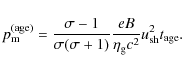
Hence, in order to obtain
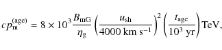
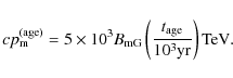
A possible solution is to consider the escape-limited acceleration. One can find from Eq. (17) that if we take
![]() pc, the maximum energy becomes
pc, the maximum energy becomes
| |
= | (31) |
which is consistent with the observed gamma-ray spectrum. Below we consider the model of escape-limited acceleration under simple assumptions, estimating the evolution of the number density and the maximum momentum of accelerated particles so as to discuss the spectral index
4.2 Evolution of pm
Time evolution of the maximum momentum of accelerated particle ![]() has been so far discussed in many contexts (e.g., Ptuskin & Zirakashvili 2003). One way to estimate
has been so far discussed in many contexts (e.g., Ptuskin & Zirakashvili 2003). One way to estimate ![]() is to use Eq. (16). In this approach, a key parameter is the magnetic field, which is likely amplified around the shock front (Bamba et al. 2005b; Yamazaki et al. 2004; Bamba et al. 2005a; Uchiyama et al. 2007; Bamba et al. 2003; Vink & Laming 2003)
and may depend on various physical quantities like the shock velocity,
the ambient density, and so on. At present, the evolution of
the magnetic field is not well understood despite many works on the
subject (e.g., Riquelme & Spitkovsky 2009; Niemiec et al. 2008; Ohira et al. 2009a; Luo & Melrose 2009).
In addition, the evolution of another parameter
is to use Eq. (16). In this approach, a key parameter is the magnetic field, which is likely amplified around the shock front (Bamba et al. 2005b; Yamazaki et al. 2004; Bamba et al. 2005a; Uchiyama et al. 2007; Bamba et al. 2003; Vink & Laming 2003)
and may depend on various physical quantities like the shock velocity,
the ambient density, and so on. At present, the evolution of
the magnetic field is not well understood despite many works on the
subject (e.g., Riquelme & Spitkovsky 2009; Niemiec et al. 2008; Ohira et al. 2009a; Luo & Melrose 2009).
In addition, the evolution of another parameter
![]() is also unknown. This prevents us from predicting
is also unknown. This prevents us from predicting ![]() rigorously.
rigorously.
Here we adopt a different phenomenological approach based on the
assumption that young SNRs are responsible for observed CRs below the
knee (Gabici et al. 2009). The maximum energy
![]() is expected to increase up to the knee energy (1015.5 eV) until the end of the free expansion phase
is expected to increase up to the knee energy (1015.5 eV) until the end of the free expansion phase
![]() and decreases from that epoch. As seen in Sect. 4.1,
and decreases from that epoch. As seen in Sect. 4.1, ![]() is limited by the escape at
is limited by the escape at
![]() ,
that is
,
that is
![]() .
Then, to reproduce the observed CR spectrum from
.
Then, to reproduce the observed CR spectrum from ![]() GeV to the knee, we may assume a functional form of
GeV to the knee, we may assume a functional form of
|
(32) |
where
|
(33) |
where
so that we have
4.3 Dynamics of SNR shock waves
In this subsection, we consider the dynamics of the SNR shock to
estimate the evolution of the normalization factor of the
spectrum
![]() .
A simple treatment of the dynamics of the SNR shock from the
free expansion to the adiabatic expansion (Sedov) phase has been given
by several authors (Drury et al. 1989; Bisnovatyi-Kogan & Silich 1995; Ostriker & McKee 1988).
Here we extend their method taking into account the cooling by
CR escape. The total mass of the SNR shock shell is
calculated as
.
A simple treatment of the dynamics of the SNR shock from the
free expansion to the adiabatic expansion (Sedov) phase has been given
by several authors (Drury et al. 1989; Bisnovatyi-Kogan & Silich 1995; Ostriker & McKee 1988).
Here we extend their method taking into account the cooling by
CR escape. The total mass of the SNR shock shell is
calculated as
where

where the gas velocity u is related to the shock velocity
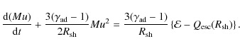
Since
![\begin{displaymath}%
\frac{\gamma_{\rm ad}+1}{4M}R_{\rm sh}^{-\omega}
\frac{{\rm d}}{{\rm d} R_{\rm sh}}\left[
R_{\rm sh}^\omega(Mu)^2\right],
\end{displaymath}](/articles/aa/full_html/2010/05/aa13495-09/img163.png)
|
(38) |
where
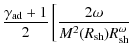
![$\displaystyle \times ~ \left. \int_0^{R_{\rm sh}} {\rm d} r ({\cal E} -Q_{\rm esc}(r))
r^{\omega -1} M(r) \right]^{1/2}.$](/articles/aa/full_html/2010/05/aa13495-09/img167.png)
Once
where
where
4.4 Evolution of K
In this subsection we discuss the evolution of the normalization factor
![]() of the spectrum of accelerated particles. At present, the
injection process for CR acceleration at the shock is not well
understood. Hence we consider two representative scenarios of the
injection process to model the amount of the accelerated particles.
of the spectrum of accelerated particles. At present, the
injection process for CR acceleration at the shock is not well
understood. Hence we consider two representative scenarios of the
injection process to model the amount of the accelerated particles.
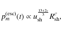
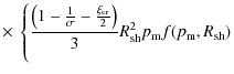
At first, we consider the same injection model as that of Ptuskin & Zirakashvili (2005). The model requires that the CR pressure at the shock is proportional to the fluid ram pressure, that is,
![]() .
The CR pressure at the shock
.
The CR pressure at the shock
![]() is given by
is given by
|
(42) |
where we neglect the contribution of non-relativistic particles. Then one can find that
|
(43) |
where we used the fact that the distribution function of CRs at the shock front is essentially
|
(44) |
where the mechanical energy of the ejecta is (up to the numerical coefficient)
|
(45) |
If the explosion is adiabatic,
![\begin{figure}
\par\includegraphics[width=8.5cm,clip]{13495fg1.eps}
\end{figure}](/articles/aa/full_html/2010/05/aa13495-09/img201.png)
|
Figure 1:
The index
|
| Open with DEXTER | |
![\begin{figure}
\par\includegraphics[width=8.5cm,clip]{13495fg2.eps}
\end{figure}](/articles/aa/full_html/2010/05/aa13495-09/img202.png)
|
Figure 2: The same as Fig. 1, but for the case PH. |
| Open with DEXTER | |
Next we consider the thermal leakage (TL) model (Malkov & Völk 1995). This model requires the continuity of the distribution function f0(p) to the downstream Maxwelian at the injection momentum
![]() , namely
, namely
|
(46) |
With this we derive
| (47) |
where
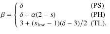
In summary, the evolution of the normalization factor of the accelerated particles spectrum is given by
![]() , with
, with
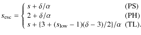
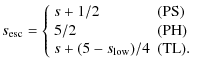
4.5 The spectrum of escaping particles
We obtain from Eqs. (27), (28), and (48) the index of the momentum spectrum of escaping particles as
|
(49) |
Now, we discuss which injection model is suitable to reproduce the galactic CR spectrum observed on Earth. We adopt
For PS
![]() is smaller than s because
is smaller than s because
![]() ,
so that the model predicts the harder spectrum of escaping particles rather than that of the source. However, since
,
so that the model predicts the harder spectrum of escaping particles rather than that of the source. However, since
![]() ,
the difference is small. In order to reproduce the observed Galactic CR spectrum
,
the difference is small. In order to reproduce the observed Galactic CR spectrum
![]() ,
the source spectrum should be
,
the source spectrum should be
![]() .
Hence the PS model requires s>2 at the source. This condition is satisfied if we consider the diffusive shock acceleration at a moderate Mach number (Fujita et al. 2009). It is also possible to derive s>2 if we consider the effects of neutral particles (Ohira et al. 2009b; Ohira & Takahara 2009).
.
Hence the PS model requires s>2 at the source. This condition is satisfied if we consider the diffusive shock acceleration at a moderate Mach number (Fujita et al. 2009). It is also possible to derive s>2 if we consider the effects of neutral particles (Ohira et al. 2009b; Ohira & Takahara 2009).
For PH, because the value of
![]() is small,
is small,
![]() is always near 2, which is the value predicted by the diffusive
shock acceleration theory in the strong shock, test-particle limit.
In particular, if
is always near 2, which is the value predicted by the diffusive
shock acceleration theory in the strong shock, test-particle limit.
In particular, if ![]() - indeed, even in the test-particle limit where the cooling via CR escape can be neglected, the value of
- indeed, even in the test-particle limit where the cooling via CR escape can be neglected, the value of ![]() is not exactly zero unless
is not exactly zero unless
![]() (see Fig. 2) - then, one can find
(see Fig. 2) - then, one can find
![]() .
This is what Berezhko & Krymsky (1998) and Ptuskin & Zirakashvili (2005) showed. Note that from Fig. 2
.
This is what Berezhko & Krymsky (1998) and Ptuskin & Zirakashvili (2005) showed. Note that from Fig. 2 ![]() is negative for a long time, so that
is negative for a long time, so that
![]() .
Therefore, model PH cannot reproduce the observed Galactic CR spectrum on Earth.
.
Therefore, model PH cannot reproduce the observed Galactic CR spectrum on Earth.
For TL, neglecting ![]() ,
we obtain
,
we obtain
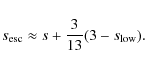
|
(50) |
Hence if
5 Application to AGN cocoon shocks
In this section, taking account of a constraint derived from the
spectrum on Earth, we study the origin of CRs with energies higher than
![]() eV and their acceleration mechanism at AGNs. There are many works which discuss UHECR production in AGNs (e.g., Berezinsky et al. 2006; Rachen & Biermann 1993; Takahara 1990; Pe'er et al. 2009; Biermann & Strittmatter 1987; Berezhko 2008).
Many of them focus on UHECR acceleration in radio galaxies
including Fanaroff-Riley (FR) I and II galaxies, which
typically have powerful jets. In the context of DSA, one can
basically suppose three acceleration zones; internal shocks in jets,
hot spots, and cocoon shocks. The former two are the most widely
discussed scenarios, but the detailed study of DSA at such mildly
relativistic shocks has not yet been achieved. We concentrate on the
cocoon shock scenario proposed by Berezhko (2008), where the non-relativistic DSA theory can be applied.
eV and their acceleration mechanism at AGNs. There are many works which discuss UHECR production in AGNs (e.g., Berezinsky et al. 2006; Rachen & Biermann 1993; Takahara 1990; Pe'er et al. 2009; Biermann & Strittmatter 1987; Berezhko 2008).
Many of them focus on UHECR acceleration in radio galaxies
including Fanaroff-Riley (FR) I and II galaxies, which
typically have powerful jets. In the context of DSA, one can
basically suppose three acceleration zones; internal shocks in jets,
hot spots, and cocoon shocks. The former two are the most widely
discussed scenarios, but the detailed study of DSA at such mildly
relativistic shocks has not yet been achieved. We concentrate on the
cocoon shock scenario proposed by Berezhko (2008), where the non-relativistic DSA theory can be applied.
In this scenario, extragalactic CRs with energies higher than the second knee (
![]() eV)
may be accelerated at the outer cocoon shock running into the
intergalactic medium (IGM). As powerful jets penetrating into a
uniform ambient medium with a density
eV)
may be accelerated at the outer cocoon shock running into the
intergalactic medium (IGM). As powerful jets penetrating into a
uniform ambient medium with a density
![]() ,
the heads of the cocoon advances into the IGM with a velocity
,
the heads of the cocoon advances into the IGM with a velocity ![]() .
At the same time, the cocoon expands sideways with a velocity
.
At the same time, the cocoon expands sideways with a velocity ![]() .
Since the typical cocoon shock is non-relativistic, we apply the
escape-limited model considered in previous sections. Although we
hereafter focus on this scenario, note that it is very uncertain
whether the efficient acceleration occurs there since the observed
non-thermal emission is much weaker than that from hot spots
and lobes.
.
Since the typical cocoon shock is non-relativistic, we apply the
escape-limited model considered in previous sections. Although we
hereafter focus on this scenario, note that it is very uncertain
whether the efficient acceleration occurs there since the observed
non-thermal emission is much weaker than that from hot spots
and lobes.
Below we investigate whether the CR spectrum above the second knee can
be explained by the AGN cocoon shock scenario with the same
parameters for young SNRs explaining the CR spectrum below the
knee, which were discussed in Sect. 4. Similar to the previous calculations in Sect. 4, we hereafter calculate the values of
![]() and
and
![]() to derive the spectral index
to derive the spectral index
![]() .
Here we adopt
.
Here we adopt ![]() ,
where
,
where ![]() is the variable which appeared in Sect. 3.3.
is the variable which appeared in Sect. 3.3.
First, let us consider the evolution of the maximum momentum
![]() in a phenomenological way. For young SNR (Sect. 4.2), we phenomenologically expect
in a phenomenological way. For young SNR (Sect. 4.2), we phenomenologically expect
![]() .
Then, by using the Sedov-Taylor solution (
.
Then, by using the Sedov-Taylor solution (
![]() and
and
![]() ), we can easily obtain
), we can easily obtain
where c is a phenomenologically introduced parameter since one can expect
In order to obtain the value of
![]() ,
the dynamics of the AGN cocoon are necessary. A simple
consideration of the cocoon dynamics for the constant density IGM
tells us that
,
the dynamics of the AGN cocoon are necessary. A simple
consideration of the cocoon dynamics for the constant density IGM
tells us that ![]() is almost time-independent and
is almost time-independent and ![]() evolves as
evolves as
![]() (Begelman & Cioffi 1989), so that the cocoon radius evolves as
(Begelman & Cioffi 1989), so that the cocoon radius evolves as
![]() and the jet radius evolves as
and the jet radius evolves as
![]() .
Then, we obtain
.
Then, we obtain
![]() and
and
![]() for c=0 and c=1, respectively.
for c=0 and c=1, respectively.
Next let us consider the time dependence of the normalization factor of the spectrum of accelerated CRs,
![]() .
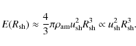
The volume of the acceleration region swept by the cocoon shock is
.
The volume of the acceleration region swept by the cocoon shock is
![]() ,
where
,
where
![]() is the total area of the shock surface. If we assume the elliptical shape of the cocoon
is the total area of the shock surface. If we assume the elliptical shape of the cocoon![]() , then
, then
![]() ,
so that
,
so that
![]() .
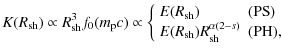
For PS and PH,
.
For PS and PH,
![]() is related to
is related to
![]() .
The dependence of
.
The dependence of
![]() is written as
is written as
![]() ,
where we neglect for simplicity the evolution of the acceleration efficiency which was considered in Berezhko (2008). Accordingly, for PS
,
where we neglect for simplicity the evolution of the acceleration efficiency which was considered in Berezhko (2008). Accordingly, for PS
![]() leads to
leads to
| (52) |
while for PH,
| (53) |
Finally, for the model TL (see Sect. 4.4),
| (54) |
where we assume the constant IGM density
With the above results we can obtain the spectrum of escaping particles. Here, we assume
|
(56) |
Interestingly, all three cases (PS, PH and TL) lead to the source spectral index
6 Summary and discussion
We investigated the escape-limited model of CR acceleration, in which the maximum energy of CRs of an accelerator is limited by the escape from the acceleration site. The typical energy of escaping CRs decreases as the shock decelerates because the diffusion length becomes longer. After revisiting the escape-limited model and reconsidering its details more generally, we derived a simple relation between the spectrum of escaping particles and that in the accelerator. Then, using the obtained relation, we discussed which model of injection is potentially suitable to make the Galactic and extragalactic CRs observed at the Earth. As discussed in the beginning of Sect. 3, there are two approaches to the maximum momentum of accelerated particles in the escape-limited model, momentum or spatial boundary. The reality is somewhere between these two extremes in any case. However, we note that once a delta-function approximation is made as in Eq. (21), the two are essentially identical.
For young SNRs we considered the shock evolution with cooling by
escaping CRs and those spectra for the three injection models.
As a result, we found that for PH, it is difficult to satisfy
the condition for the source spectrum of Galactic CRs (
![]() ). On the other hand,
). On the other hand,
![]() can be achieved for PS and TL.
can be achieved for PS and TL.
We also applied our escape-limited model to AGN cocoon shocks as
well as young SNRs. This model is just one of the various candidates
proposed so far, even if AGNs are UHECR accelerators.
Nevertheless, it is interesting that the young SNR and the AGN
cocoon shock scenarios can explain the Galactic and extragalactic
cosmic rays observed on Earth in the same picture for all the three
injection models if we accept the proton-dip model inferring
![]() .
Whether the proton dip model is real or not can also be tested by
future UHECR and high-energy neutrino observations. We focused on the
proton case. Obviously, heavier nuclei become important above the knee
so that we need to take them into account to explain the
CR spectrum over the whole energy range. We can also apply the
escape-limited model to heavy nuclei CRs for this purpose, although
this is beyond the scope of this paper.
.
Whether the proton dip model is real or not can also be tested by
future UHECR and high-energy neutrino observations. We focused on the
proton case. Obviously, heavier nuclei become important above the knee
so that we need to take them into account to explain the
CR spectrum over the whole energy range. We can also apply the
escape-limited model to heavy nuclei CRs for this purpose, although
this is beyond the scope of this paper.
We point out a potential problem for the magnetic field amplification in the escape-limited model.
For young SNRs, we determined the evolution of the maximum energy in the phenomenological way, and adopted
![]() .
With Eqs. (16) and (51), we obtained
.
With Eqs. (16) and (51), we obtained
![]() ,
where
,
where
![]() .
The same result is obtained for AGN cocoon shocks because we
considered the case in which the same parameters describe both the
young SNR shocks and the AGN cocoon shocks.
In particular, for c =1 as used in Eq. (31), we obtained
.
The same result is obtained for AGN cocoon shocks because we
considered the case in which the same parameters describe both the
young SNR shocks and the AGN cocoon shocks.
In particular, for c =1 as used in Eq. (31), we obtained
![]() ,
which means that B rapidly decreases with radius (or time). In principle, both the dependence of B on
,
which means that B rapidly decreases with radius (or time). In principle, both the dependence of B on
![]() and the value of c can be determined theoretically, and then the evolution of the maximum energy should be predicted.
Some previous works are based on theoretical arguments on the magnetic field evolution (e.g., Bell 2004; Caprioli et al. 2009; Berezhko 2008; Pelltier et al. 2006),
which seem to be different from our phenomenological one.
At present, the mechanisms of the particle acceleration and the
magnetic field amplification are still highly uncertain despite many
theoretical efforts (e.g., Riquelme & Spitkovsky 2009; Niemiec et al. 2008; Ohira et al. 2009a; Luo & Melrose 2009).
Hence we expect that further theoretical and observational studies can
resolve this discrepancy or exclude the possibility of escape-limited
acceleration in the future.
and the value of c can be determined theoretically, and then the evolution of the maximum energy should be predicted.
Some previous works are based on theoretical arguments on the magnetic field evolution (e.g., Bell 2004; Caprioli et al. 2009; Berezhko 2008; Pelltier et al. 2006),
which seem to be different from our phenomenological one.
At present, the mechanisms of the particle acceleration and the
magnetic field amplification are still highly uncertain despite many
theoretical efforts (e.g., Riquelme & Spitkovsky 2009; Niemiec et al. 2008; Ohira et al. 2009a; Luo & Melrose 2009).
Hence we expect that further theoretical and observational studies can
resolve this discrepancy or exclude the possibility of escape-limited
acceleration in the future.
We mainly considered spectra of dispersed CRs around young SNRs and
AGN cocoon shocks. However, applications to other astrophysical
objects are, of course, possible. For example, the old SNRs
detected by Fermi LAT, like W28, W44, W51 and IC 443 (Abdo et al. 2009b,a)
have been of great interest because they likely generate escaping CRs.
In fact, the number of CRs around these old SNRs is likely to
decrease with time or the shock radius, that is ![]() while
while ![]() .
For example, when we consider the dynamics of an old SNR, we have
.
For example, when we consider the dynamics of an old SNR, we have
![]() (e.g., Yamazaki et al. 2006), so that we have
(e.g., Yamazaki et al. 2006), so that we have
![]() ,
i.e.,
,
i.e.,
![]() .
On the other hand, the value of
.
On the other hand, the value of ![]() may be different from 6.5, which could be attributed to various
complications like the interaction with the dense molecular cloud, and
so on. For example, for the maximum hardening case,
that is,
may be different from 6.5, which could be attributed to various
complications like the interaction with the dense molecular cloud, and
so on. For example, for the maximum hardening case,
that is,
![]() (see Appendix A.2), we find
(see Appendix A.2), we find
![]() when
when
![]() and
and
![]() where we assume
where we assume
![]() .
This might be the case for old SNRs such as W51C (Abdo et al. 2009b). In addition, the maximum energy may be rather small for the old SNRs, so that the spectrum above
.
This might be the case for old SNRs such as W51C (Abdo et al. 2009b). In addition, the maximum energy may be rather small for the old SNRs, so that the spectrum above
![]() would be suppressed. The spectrum of high-energy gamma rays could give
us important information on both the acceleration and escape processes
of CRs with energies much lower than the knee energy.
would be suppressed. The spectrum of high-energy gamma rays could give
us important information on both the acceleration and escape processes
of CRs with energies much lower than the knee energy.
We thank Akira Okumura and Yutaka Fujita for useful comments. We also thank the referee, Luke Drury, for valuable comments to improve the paper. Y.O. and K.M. acknowledge Grant-in-Aid from JSPS. This work was supported in part by grant-in-aid from the Ministry of Education, Culture, Sports, Science, and Technology (MEXT) of Japan, No. 19047004, No. 21740184, No. 21540259 (R. Y.).
Appendix A: Effect of adiabatic loss on the spectrum of escaping CRs
The instantaneous spectrum of CRs escaping from the acceleration site when the shock radius
![]() is obtained from Eq. (23) of Ptuskin & Zirakashvili (2005),
is obtained from Eq. (23) of Ptuskin & Zirakashvili (2005),
where
|
(A.2) |

|
(A.3) |
where A is a normalization factor of the distribution function, and p and
and we solve the following equation
|
(A.5) |
Then one can get the following solution
|
(A.6) |
Therefore the total spectrum of escaping CRs is
| (A.7) |
where
|
(A.8) |
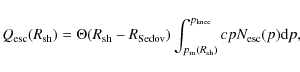
The
![$\displaystyle \qquad \qquad \left\{ \begin{array}{ll}
R^{\sigma(s+\beta-1)-s+1}...
...\left(s-1\right)\left(\frac{1}{\sigma}-1\right)\right], \\
\end{array} \right.$](/articles/aa/full_html/2010/05/aa13495-09/img315.png)
where R0 is the radius at which
A.1

In this case, the ![]() integral of Eq. (A.9)
is dominated by the outer region, that is, the spectrum of escaping
particles does not depend on the past acceleration history.
integral of Eq. (A.9)
is dominated by the outer region, that is, the spectrum of escaping
particles does not depend on the past acceleration history.
![]() is calculated as
is calculated as
| |
= | 
|
|
|
|||
| = | 
|
(A.11) |
Hence, as long as
A.2

In this case, the ![]() integral of Eq. (A.9)
is dominated by the inner region, that is, the spectrum of
escaping particles depends on the past acceleration history.
Especially, only the acceleration at
integral of Eq. (A.9)
is dominated by the inner region, that is, the spectrum of
escaping particles depends on the past acceleration history.
Especially, only the acceleration at
![]() is important, and then
is important, and then
![]() is calculated as
is calculated as
| |
= | 
|
|
|
|||
| = | 
|
(A.12) |
Because
|
(A.13) |
where we assume the relation between the spectrum index and the compression ratio,
References
- Abdo, A. A., Ackermann, M., Ajello, M., et al. 2009a, ApJS, 183, 46 [CrossRef] [Google Scholar]
- Abdo, A. A., Ackermann, M., Ajello, M., et al. 2009b, ApJ, 706, L1 [Google Scholar]
- Aharonian, F. A., & Atoyan, A. M. 1999, A&A, 351, 330 [NASA ADS] [Google Scholar]
- Aharonian, F. A., Akhperjanian, A. G., Aye, K.-M., et al. 2004, Nature, 432, 75 [NASA ADS] [CrossRef] [PubMed] [Google Scholar]
- Aharonian, F., Akhperjanian, A. G., Bazer-Bachi, A. R., et al. 2005, A&A, 437, L7 [NASA ADS] [CrossRef] [EDP Sciences] [Google Scholar]
- Aharonian, F., Akhperjanian, A. G., Bazer-Bachi, A. R., et al. 2006, A&A, 449, 223 [NASA ADS] [CrossRef] [EDP Sciences] [Google Scholar]
- Aharonian, F., Akhperjanian, A. G., Bazer-Bachi, A. R., et al. 2007, A&A, 464, 235 [Google Scholar]
- Aloisio, R., Berezinsky, V., Blasi, P., et al. 2007, Astropart. Phys., 27, 76 [NASA ADS] [CrossRef] [Google Scholar]
- Arons, J. 2003, ApJ, 589, 871 [NASA ADS] [CrossRef] [Google Scholar]
- Axford, W. I., Leer, E., & Skadron, G. 1977, Proc. 15th Int. Cosmic Ray Conf., Plovdiv, 11, 132 [Google Scholar]
- Bamba, A., Yamazaki, R., Ueno, M., & Koyama, K. 2003, ApJ, 589, 827 [NASA ADS] [CrossRef] [Google Scholar]
- Bamba, A., Yamazaki, R., Yoshida, T., Terasawa, T., & Koyama, K. 2005a, ApJ, 621, 793 [NASA ADS] [CrossRef] [Google Scholar]
- Bamba, A., Yamazaki, R., & Hiraga, J. S. 2005b, ApJ, 632, 294 [NASA ADS] [CrossRef] [Google Scholar]
- Begelman, M. C., & Cioffi, D. F. 1989, ApJ, 345, L21 [NASA ADS] [CrossRef] [Google Scholar]
- Bell, A. R. 1978, MNRAS, 182, 147 [NASA ADS] [CrossRef] [Google Scholar]
- Bell, A. R. 2004, MNRAS, 353, 550 [Google Scholar]
- Berezhko, E. G. 2008, ApJ, 684, L69 [NASA ADS] [CrossRef] [Google Scholar]
- Berezhko, E. G., & Ellison, D. C. 1999, ApJ, 526, 385 [NASA ADS] [CrossRef] [Google Scholar]
- Berezhko, E. G., & Krymsky, G. F. 1988, Soviet Phys.-Uspekhi, 12, 155 [Google Scholar]
- Berezinsky, V., Gazizov, A., & Grigorieva, S. 2006, Phys. Rev. D, 74, 043005 [NASA ADS] [CrossRef] [Google Scholar]
- Biermann, P. L., & Strittmatter, P. A. 1987, ApJ, 322, 643 [NASA ADS] [CrossRef] [Google Scholar]
- Blandford, R. D., & Ostriker, J. P. 1978, ApJ, 221, L29 [Google Scholar]
- Bisnovatyi-Kogan, G. S., & Silich, S. A. 1995, Rev. Mod. Phys., 67, 661 [NASA ADS] [CrossRef] [Google Scholar]
- Blandford, R. D., & Eichler, D. 1987, Phys. Rep., 154,1 [Google Scholar]
- Butt, Y. 2008, MNRAS, 386, L20 [NASA ADS] [CrossRef] [Google Scholar]
- Caprioli, D., Blasi, P., & Amato, E. 2009, MNRAS, 396, 2065 [NASA ADS] [CrossRef] [Google Scholar]
- Cronin, J. W. 1999, Rev. Mod. Phys., 71, S165 [CrossRef] [Google Scholar]
- Drury, L. O'C. 1983, Rep. Prog. Phys., 46, 973 [NASA ADS] [CrossRef] [Google Scholar]
- Drury, L. O'C., & Völk, H. J. 1981, ApJ, 248, 344 [NASA ADS] [CrossRef] [Google Scholar]
- Drury, L. O'C., Markiewicz, W. J., & Voelk, H. J. 1989, A&A, 225, 179 [NASA ADS] [Google Scholar]
- Drury, L. O'C., Aharonian, F. A., Malyshev, D., & Gabici, S. 2009, A&A, 496, 1 [NASA ADS] [CrossRef] [EDP Sciences] [Google Scholar]
- Enomoto, R., Tanimori, T., Naito, T., et al. 2002, Nature, 416, 823 [NASA ADS] [CrossRef] [PubMed] [Google Scholar]
- Fujita, Y., Kohri, K., Yamazaki, R., & Kino, M. 2007, ApJ, 663, L61 [NASA ADS] [CrossRef] [Google Scholar]
- Fujita, Y., Ohira, Y., Tanaka, S. J., & Takahara, F. 2009, ApJ, 707, L179 [NASA ADS] [CrossRef] [Google Scholar]
- Gabici, S., Aharonian, F. A., & Casanova, S. 2009, MNRAS, 396, 1629 [NASA ADS] [CrossRef] [Google Scholar]
- Giacalone, J., & Jokipii, J. A. 2007, ApJ, 663, L41 [NASA ADS] [CrossRef] [Google Scholar]
- Helder, E. A., Vink, J., Bassa, C. G., et al. 2009, Science, 325, 719 [NASA ADS] [CrossRef] [PubMed] [Google Scholar]
- Inoue, S., Sigl, G., Miniati, F., & Armengaud, E. 2007, Proceedings of the 30th ICRC, Merida, Mexico [arXiv:0711.1027] [Google Scholar]
- Inoue, T., Yamazaki, R., & Inutsuka, S. 2009, ApJ, 695, 825 [NASA ADS] [CrossRef] [Google Scholar]
- Kang, H., Rachen, J. P., & Biermann, P. L. 1997, MNRAS, 286, 257 [NASA ADS] [Google Scholar]
- Kang, H., Jones, T. W., LeVeque, R. J., & Shyue, K. M. 2001, ApJ, 550, 737 [NASA ADS] [CrossRef] [Google Scholar]
- Kachelriess, M., & Semikoz, D. V. 2006, Phys. Lett. B, 634, 143 [NASA ADS] [CrossRef] [Google Scholar]
- Katagiri, H., Enomoto, R., Ksenofontov, L. T., et al. 2005, ApJ, 619, L163 [NASA ADS] [CrossRef] [Google Scholar]
- Katz, B., & Waxman, E. 2008, J. Cosmology Astropart. Phys., 01, 018 [Google Scholar]
- Krymsky, G. F. 1977, Doki. Akad. Nauk SSSR, 234, 1306 [Google Scholar]
- Lucek, S. G., & Bell, A. R. 2000, MNRAS, 314, 65 [NASA ADS] [CrossRef] [Google Scholar]
- Luo, Q., & Melrose, D. 2009, MNRAS, 397, 1402 [NASA ADS] [CrossRef] [Google Scholar]
- Malkov, M. A. 1997, ApJ, 485, 638 [NASA ADS] [CrossRef] [Google Scholar]
- Malkov, M. A., & Völk, H. J. 1995, A&A, 300, 605 [NASA ADS] [Google Scholar]
- Malkov, M. A., & Drury, L. O'C. 2001, Rep. Prog. Phys., 64, 429 [NASA ADS] [CrossRef] [Google Scholar]
- Murase, K., Ioka, K., Nagataki, S., & Nakamura, T. 2006, ApJ, 651, L5 [NASA ADS] [CrossRef] [Google Scholar]
- Murase, K., Inoue, S., & Nagataki, S. 2008, ApJ, 689, L105 [NASA ADS] [CrossRef] [Google Scholar]
- Murase, K., Mészáros, P., & Zhang, B. 2009, Phys. Rev. D, 79, 103001 [NASA ADS] [CrossRef] [Google Scholar]
- Niemiec, J., Pohl, M., Stroman, T., & Nishikawa, K. 2008, ApJ684, 1174 [NASA ADS] [CrossRef] [Google Scholar]
- Ohira, Y., & Takahara, F. 2009 [arXiv:0912.2859] [Google Scholar]
- Ohira, Y., Reville, B., Kirk, J. G., & Takahara, F. 2009a, ApJ, 698, 445 [NASA ADS] [CrossRef] [Google Scholar]
- Ohira, Y., Terasawa, T., & Takahara, F. 2009b, ApJ, 703, L59 [NASA ADS] [CrossRef] [Google Scholar]
- Ostriker, J. P., & McKee, C. F. 1988, Rev. Mod. Phys., 60, 1 [NASA ADS] [CrossRef] [Google Scholar]
- Pelltier, G., Lemoine, M., & Marcowith, A. 2006, A&A, 453, 181 [NASA ADS] [CrossRef] [EDP Sciences] [Google Scholar]
- Parizot, E., Marcowith, A., Ballet, J., & Gallant, Y. A. 2006, A&A, 453, 387 [NASA ADS] [CrossRef] [EDP Sciences] [Google Scholar]
- Pe'er, A., Murase, K., & Mészáros, P. 2009, Phys. Rev. D., 80, 123018 [Google Scholar]
- Plaga, R. 2008, New A. 13, 73 [Google Scholar]
- Ptuskin, V. S., & Zirakashvili, V. N. 2003, A&A, 403, 1 [NASA ADS] [CrossRef] [EDP Sciences] [Google Scholar]
- Ptuskin, V. S., & Zirakashvili, V. N. 2005, A&A, 429, 755 [NASA ADS] [CrossRef] [EDP Sciences] [MathSciNet] [PubMed] [Google Scholar]
- Putze, A., Derome, L., Maurin, D., Perotto, L., & Taillet, R. 2009, A&A, 497, 991 [NASA ADS] [CrossRef] [EDP Sciences] [Google Scholar]
- Rachen, J. P., & Biermann, P. L. 1993, A&A, 272, 161 [NASA ADS] [Google Scholar]
- Reville, B., Kirk, J. G., Duffy, P., & O'Sullivan, S. 2007, A&A, 475, 435 [NASA ADS] [CrossRef] [EDP Sciences] [Google Scholar]
- Reville, B., Kirk, J. G., & Duffy, P. 2009, ApJ, 694, 951 [NASA ADS] [CrossRef] [Google Scholar]
- Reynolds, S. P. 1998, ApJ, 493, 375 [NASA ADS] [CrossRef] [Google Scholar]
- Riquelme, M. A., & Spitkovsky, A. 2009, ApJ, 694, 626 [Google Scholar]
- Strong, A. W., & Moskalenko, I. V. 1998, ApJ, 509, 212 [NASA ADS] [CrossRef] [Google Scholar]
- Strong, A. W., Moskalenko, I. V., & Reimer, O. 2000, ApJ, 537, 763 [Google Scholar]
- Takahara, F. 1990, Prog. of Theo. Phys., 83, 1071 [Google Scholar]
- Tanaka, T., Uchiyama, Y., Aharonian, F. A., et al. 2008, ApJ, 685, 988 [NASA ADS] [CrossRef] [Google Scholar]
- Uchiyama, Y., Aharonian, F. A., Tanaka, T., Takahashi, T., & Maeda, Y. 2007, Nature, 449, 576 [NASA ADS] [CrossRef] [PubMed] [Google Scholar]
- Vietri, M. 1995, ApJ, 453, 883 [Google Scholar]
- Villante, F. L., & Vissani, F. 2007, Phys. Rev. D, 76, 125019 [Google Scholar]
- Vink, J., & Laming, J. M. 2003, ApJ, 584, 758 [NASA ADS] [CrossRef] [Google Scholar]
- Völk, H. J., Berezhko, E. G., & Ksenofontov, L. T. 2008, A&A, 483, 529 [NASA ADS] [CrossRef] [EDP Sciences] [Google Scholar]
- Wang, X.-Y., Razzaque, S., Mészáros, & Dai, Z.-G. 2007, Phys. Rev. D, 76, 083009 [NASA ADS] [CrossRef] [Google Scholar]
- Warren, J. S., Hughes, J. P., Badenes, C., et al. 2005, ApJ, 634, 376 [NASA ADS] [CrossRef] [Google Scholar]
- Waxman, E. 1995, Phys. Rev. Lett., 75, 386 [NASA ADS] [CrossRef] [PubMed] [Google Scholar]
- Yamazaki, R., Yoshida, T., Terasawa, T., Bamba, A., & Koyama, K. 2004, A&A, 416, 595 [NASA ADS] [CrossRef] [EDP Sciences] [Google Scholar]
- Yamazaki, R., Kohri, K., Bamba, A., et al. 2006, MNRAS, 371, 1975 [NASA ADS] [CrossRef] [Google Scholar]
- Yamazaki, R., Kohri, K., & Katagiri, H. 2009, A&A, 495, 9 [NASA ADS] [CrossRef] [EDP Sciences] [Google Scholar]
Footnotes
- ...

![[*]](/icons/foot_motif.png)
- We search for approximate solutions to Eqs. (39), (41)
and (48),
which determine
 (and
(and  )
for given parameters
)
for given parameters  , s,
, s,  and
and
 .
The procedure is as follows. For a trial value of
which is assumed to be constant, we solve Eqs. (39)
and (41)
to obtain
.
The procedure is as follows. For a trial value of
which is assumed to be constant, we solve Eqs. (39)
and (41)
to obtain  so as to calculate E and
as functions of
so as to calculate E and
as functions of
 .
It is found that
is almost time-independent after
.
It is found that
is almost time-independent after
 ,
hence we can derive its average value in the epoch
,
hence we can derive its average value in the epoch  .
Then we update the value of
with Eq. (48)
with the average value of .
We repeat this procedure until the iteration converges.
.
Then we update the value of
with Eq. (48)
with the average value of .
We repeat this procedure until the iteration converges.
- ... cocoon
- Berezhko (2008)
assumed a kind of spherical cocoon, i.e.,
 ,
and used
,
and used  which is similar to the relation obtained for the model PS.
However, when the cocoon becomes spherical,
which is similar to the relation obtained for the model PS.
However, when the cocoon becomes spherical,  and
and  evolve according to the adiabatic solution as in the Sedov-Taylor
solution for SNRs (Fujita
et al. 2007; Begelman & Cioffi 1989).
evolve according to the adiabatic solution as in the Sedov-Taylor
solution for SNRs (Fujita
et al. 2007; Begelman & Cioffi 1989).
- ... density
- However, it may not be the case since the
IGM density may drop with the distance from the nucleus. Then
we need to use different adiabatic solutions for
and
 .
.
All Figures
|
|
Figure 1:
The index
|
| Open with DEXTER | |
| In the text | |
|
|
Figure 2: The same as Fig. 1, but for the case PH. |
| Open with DEXTER | |
| In the text | |
Copyright ESO 2010
Current usage metrics show cumulative count of Article Views (full-text article views including HTML views, PDF and ePub downloads, according to the available data) and Abstracts Views on Vision4Press platform.
Data correspond to usage on the plateform after 2015. The current usage metrics is available 48-96 hours after online publication and is updated daily on week days.
Initial download of the metrics may take a while.