| Issue |
A&A
Volume 513, April 2010
|
|
|---|---|---|
| Article Number | A32 | |
| Number of page(s) | 17 | |
| Section | Cosmology (including clusters of galaxies) | |
| DOI | https://doi.org/10.1051/0004-6361/200913464 | |
| Published online | 20 April 2010 | |
The mixing and transport properties of the intra cluster medium: a numerical study using tracers particles
F. Vazza1 - C. Gheller2 - G. Brunetti1
1 - INAF/Istituto di Radioastronomia, via Gobetti 101, 40129 Bologna, Italy
2 - CINECA, High Performance System Division, Casalecchio di Reno, Bologna, Italy
Received 13 October 2009 / Accepted 17 January 2010
Abstract
We present a study of the mixing properties of the simulated intra
cluster medium, using tracers particles that are advected by the gas
flow during the evolution of cosmic structures. Using a sample of seven
galaxy clusters (with masses in the range of
![]()
![]()
![]() )
simulated with a peak resolution of
)
simulated with a peak resolution of
![]() up to the distance of two virial radii from their centers, we
investigate the application of tracers to some important problems
concerning the mixing of the ICM. The transport properties of the
evolving ICM are studied through the analysis of pair dispersion
statistics and mixing distributions. As an application, we focus
on the transport of metals in the ICM. We adopt simple scenarios
for the injection of metal tracers in the ICM, and find remarkable
differences of metallicity profiles in relaxed and merger systems also
through the analysis of simulated emission from Doppler-shifted
Fe XXIII lines.
up to the distance of two virial radii from their centers, we
investigate the application of tracers to some important problems
concerning the mixing of the ICM. The transport properties of the
evolving ICM are studied through the analysis of pair dispersion
statistics and mixing distributions. As an application, we focus
on the transport of metals in the ICM. We adopt simple scenarios
for the injection of metal tracers in the ICM, and find remarkable
differences of metallicity profiles in relaxed and merger systems also
through the analysis of simulated emission from Doppler-shifted
Fe XXIII lines.
Key words: intergalactic medium - large-scale structure of Universe - turbulence - methods: numerical - hydrodynamics
1 Introduction
The mixing properties of the intra cluster medium (ICM) are still poorly understood and a number of open fields of research are tightly connected to this important topic: the ``heating cooling flows'' problem (e.g. Bruggen & Kaiser 2002; Omma et al. 2004), the spreading of metals in the ICM (e.g. Schindler & Diaferio 2008; Borgani et al. 2008), the stability of thermal profiles in the innermost region of galaxy clusters (e.g. Sharma et al. 2009), the efficiency in the ram pressure stripping of accreting satellites and the emergence of cold fronts in galaxy clusters (e.g. Ascasibar & Markevitch 2006; Markevitch & Vikhlinin 2007) and many others.
From the theoretical point of view, in the last few years meaningful
progress has been made in understanding the convective properties of
the ICM. Focusing on the role played by instabilities in a magnetized,
low-collisional plasma (e.g. Parrish & Stone 2005; Quataert 2008; Ruszkowski & Oh 2009),
a new picture of the ICM stability was presented, which
drastically alters the ``classic'' picture provided by the
Schwarzschild criterion, in which stability is ensured by
![]() > 0 (Schwarzschild 1959), where S is the specific entropy.
> 0 (Schwarzschild 1959), where S is the specific entropy.
These approaches cannot take into account all sources of mixing motions
in galaxy clusters though, which are due to large scale accretions of
matter and turbulent motions. Indeed there is clear evidence nowadays
that a sizable amount of turbulent motions may be present in the ICM.
Observations suggest large scale subsonic turbulent motions in the
range of
![]() (e.g. Schuecker et al. 2004; Henry et al. 2004;
Churazov et al. 2004). In addition, also studies of Faraday
Rotation allow a complementary approach and suggest that the
ICM magnetic field is tangled over a broad range of scales
(e.g. Murgia et al. 2004; Vogt & Ensslin 2005; Kuchar & Ensslin 2009; Bonafede et al. 2010; Vacca et al. 2010);
also, the diffuse radio emission detected in a fraction of merging
clusters may provide indirect evidence for turbulence in the ICM
(e.g. Brunetti et al. 2008).
(e.g. Schuecker et al. 2004; Henry et al. 2004;
Churazov et al. 2004). In addition, also studies of Faraday
Rotation allow a complementary approach and suggest that the
ICM magnetic field is tangled over a broad range of scales
(e.g. Murgia et al. 2004; Vogt & Ensslin 2005; Kuchar & Ensslin 2009; Bonafede et al. 2010; Vacca et al. 2010);
also, the diffuse radio emission detected in a fraction of merging
clusters may provide indirect evidence for turbulence in the ICM
(e.g. Brunetti et al. 2008).
Obtaining a self-consistent picture of the evolving ICM, where large scale and small scale mixing properties of galaxy clusters are followed during the whole cluster evolution is challenging, and in this respect cosmological high resolution numerical simulations may provide additional and valuable information.
At present, two main numerical methods are massively applied to cosmological numerical simulations: Lagrangian methods, which sample both the Dark Matter and the gas properties using unstructured point-like fluid elements, usually regarded as particles (e.g. smoothed particles hydrodynamic codes such as GADGET, Springel 2005, or HYDRA, Couchman et al. 1995) and Eulerian methods, which reconstruct the gas properties with a discrete sampling of the space using meshes of various resolution (e.g. cosmological TVD code, Ryu et al. 1993; ENZO, Norman et al. 2007; FLASH, Fryxell et al. 2000; RAMSES, Teyssier 2002, etc.) and model the Dark Matter properties with a particle mesh approach.
The typical advantages and drawbacks of the two approaches have been extensively investigated. Lagrangian methods allow one to obtain a high spatial resolution where matter concentrates, but in low density regions the sampling is rather poor. By construction, this class of methods allows one to follow in a natural way the advection of a single parcel of (gas or DM) matter during the whole simulation and its dynamical evolution.
Eulerian methods have a spatial resolution fixed to the size of the cell in the computational mesh, and this often is inadequate to follow the details of cosmological and physical processes of interest in the innermost region of collapsed objects. The adaptive mesh refinement technique (AMR) overcomes this problem by increasing the spatial resolution of the Eulerian mesh in regions of particular interest (e.g. Berger & Oliger 1984; Berger & Colella 1989; Kravtsov et al. 1997). A further important feature of Eulerian methods is that they are strictly conservative for the total fluid energy, and therefore they accurately follow the Rankine-Hugoniot relations for shocks (a property shared by shock capturing methods, also known as Godunov schemes, Godunov 1959). This is particular important in cosmological simulations, where cosmic shocks play an important role in setting both thermal and non thermal properties of the ICM (e.g. Ryu et al. 2003; Pfrommer et al. 2006; Vazza et al. 2009a,b).
In the last few years a number of works highlighted and investigated the causes which lead to the main differences between these numerical approaches (Agertz et al. 2006; Tasker et al. 2008; Wadsley et al. 2008; Mitchell et al. 2009; Robertson et al. 2010; Springel 2009). The adoption of artificial viscosity by SPH and the limited spatial resolution for AMR, were the reasons for the more significant differences between the two approaches; if however both sources of error are tuned appropriately (e.g. by reducing the action of artificial viscosity outside shocks in SPH, or by increasing the mesh resolution in AMR codes), the two approaches produce consistent results.
High resolution AMR simulations (such as the ENZO simulations presented in this paper) can provide an accurate representation of the cosmic gas dynamics in galaxy clusters, achieving a very broad dynamical range. Recent works showed that opportune refinements (e.g. Iapichino & Niemeyer 2008; Vazza et al. 2009a,b; Maier et al. 2009; Zhu et al. 2010) allow for efficiently studying the onset and evolution of chaotic motions in the ICM.
Yet, some interesting information of Lagrangian nature cannot be followed by these methods. One example is the distribution of metals in the ICM due to diffusion and turbulent mixing which cannot be followed, unless the conservation equations are self-consistently implemented for every metal species, with a sizable increase in algorithmic complexity and computational expense. However, it is possible to treat metals in a post-processing stage by following their spatial evolution through that of mass-less particles (tracers), which move along with the baryon gas.
An other interesting case is the advection of cosmic rays (CR)
particles in the ICM. Shocks, turbulence, collisions between high
energy hadrons and AGN/supernovae activities are expected to inject
relativistic particles in the ICM over cosmological time-scales
(e.g. Brunetti & Lazarian 2007), whose interplay with diffuse
![]() ICM magnetic fields is responsible for the diffuse non-thermal
radio emissions observed in galaxy clusters (e.g. Ferrari
et al. 2008,
for a recent review). If the energy stored in CR is much smaller
than the thermal ICM (as shown by recent observations of the
central regions of clusters, e.g. Reimer 2004; Aharonian et al. 2008; Brunetti et al. 2007;
THE MAGIC collaboration et al. 2009), the spatial evolution of CR
can be studied through that of passive tracers. This applies as long as
the effect of CR diffusion is negligible and the evolution of
CR particles can be regarded as the simple advection problem of
tracers in the evolving ICM.
ICM magnetic fields is responsible for the diffuse non-thermal
radio emissions observed in galaxy clusters (e.g. Ferrari
et al. 2008,
for a recent review). If the energy stored in CR is much smaller
than the thermal ICM (as shown by recent observations of the
central regions of clusters, e.g. Reimer 2004; Aharonian et al. 2008; Brunetti et al. 2007;
THE MAGIC collaboration et al. 2009), the spatial evolution of CR
can be studied through that of passive tracers. This applies as long as
the effect of CR diffusion is negligible and the evolution of
CR particles can be regarded as the simple advection problem of
tracers in the evolving ICM.
The objective of the present work is to investigate the mixing properties of the ICM with an appropriate numerical recipe. For this purpose high algorithmic accuracy and high spatial and mass resolution are needed. These requirements are well provided by ENZO, which is a high-order and cosmological AMR Eulerian code (e.g. Norman et al. 2007). Here we present ENZO simulations with two important customizations: first, an additional refinement criterion is added to increase the spatial resolution on propagating shocks (Vazza et al. 2009a,b); second, since a pure Eulerian method cannot provide the details on the behavior of each specific fluid element (e.g. its trajectory and velocity), we explicitly follow the advection of a large number of Lagrangian passive (mass-less) tracer particles, which move according to the 3D velocity field of the gas.
The paper is organized as follows: in Sect. 2 we present the details of the simulation runs for this project, and the method to inject and follow tracers. In Sect. 3 we discuss the result of several convergence tests to assess the reliability of tracers simulation with different possible setups. In Sect. 4 we present astrophysical results of tracers, studying in particular the average transport properties of tracers in all simulated clusters by discussing the evolution of the pair dispersion statistics (Sect. 4.1); the morphology and the evolution of radial mixing in merging and non merging clusters through the evolution of tracers initially located in spherical shells (Sect. 4.2); the spreading of metal tracers in the ICM, studying toy models of metal injections from galaxies (Sect. 4.3); the simulated emissivity from the broadened Fe XXIII line from metal tracers and its dependence on the the dynamical history of clusters (Sect. 4.4). Our conclusions are given in Sect. 5.
2 Numerical methods
2.1 The ENZO code
ENZO is an AMR cosmological hybrid code originally written by Bryan & Norman (Bryan & Norman 1997; Norman et al. 2007).
It uses a particle-mesh N-body method (PM) to follow the dynamics of the collision-less Dark Matter (DM) component (Hockney & Eastwood 1981). The DM component is coupled to the baryonic matter (gas), via gravitational forces, calculated from the total mass distribution (DM+gas) solving the Poisson equation with a FFT based approach.
The gas component is described as a perfect fluid, and its dynamics are calculated by solving the conservation equations of mass, energy and momentum over a computational mesh with an Eulerian solver based on the Piecewise Parabolic Method (PPM, Woodward & Colella 1984). The PPM algorithm belongs to a class of schemata in which shock waves are accurately described by building into the numerical method the calculation of the propagation and interaction of non-linear waves with a directionally split approach. It is a higher order extension of Godunov's shock capturing method (Godunov 1959). It is at least second-order accurate in space (up to the fourth-order in 1D, for smooth flows and small time-steps) and second-order accurate in time. The PPM method requires no artificial viscosity, which leads to an optimal treatment of energy conversion processes, to the minimization of errors due to the finite size of the cells of the grid and to a spatial resolution close to the nominal one. The basic PPM technique has been modified to include the gravitational interaction and the expansion of the Universe (e.g. Bryan et al. 1995). In ENZO cosmological simulations, several comparison tests (e.g. O'Shea et al. 2005; Tasker et al. 2008) provided evidence of the better performance of the PPM method implemented, compared to the alternative method of ZEUS artificial viscosity (which is also implemented in ENZO).
2.2 Cluster simulations
For the simulations presented here, we assumed a ``concordance'' ![]() CDM cosmology with the parameters
CDM cosmology with the parameters
![]() ,
,
![]() ,
,
![]() ,
,
![]() ,
the Hubble parameter h = 0.72 and a normalization for the primordial density power spectrum
,
the Hubble parameter h = 0.72 and a normalization for the primordial density power spectrum
![]() .
.
The clusters considered in this paper were extracted from independent cosmic volumes, each with the size of
![]() ,
obtained with root grids of 2563 cells and with DM mass resolution of
,
obtained with root grids of 2563 cells and with DM mass resolution of
![]()
![]()
![]() .
We additionally sub-sampled cubic volumes of side
.
We additionally sub-sampled cubic volumes of side
![]() with a second 2563 grid around the region of the formation of our clusters, achieving an effective root grid resolution of
with a second 2563 grid around the region of the formation of our clusters, achieving an effective root grid resolution of
![]() and an effective DM mass resolution of
and an effective DM mass resolution of
![]()
![]()
![]() .
For every cluster run, we identified cubic regions of the size of
.
For every cluster run, we identified cubic regions of the size of
![]() (where
(where
![]() is the virial
radius of clusters at z=0), and allowed for three additional levels of mesh refinement,
achieving a peak spatial resolution of
is the virial
radius of clusters at z=0), and allowed for three additional levels of mesh refinement,
achieving a peak spatial resolution of
![]()
![]() .
.
The mesh refinement was triggered by gas or DM over-density criteria from the beginning of all simulations (z=30). From z=2 an additional refinement criterion based on 1D velocity jumps was switched on (Vazza et al. 2009a,b). This second AMR criterion is designed to capture shocks and intense turbulent motions in the ICM out to the external cluster regions. The grid was refined of a factor two whenever one of the following conditions was matched:
- either the gas or the DM density at a given cell exceeded
 ,
where
,
where  is the gas (DM) density within the cell at the l-AMR level, and
 is the mean gas (DM) density at the root grid level (in the AMR region);
- the 1D velocity jump across a patch of three cells
(normalized to the minimum velocity modulus in the same patch) was
larger than a threshold
 ,
where i=x,y or z.
,
where i=x,y or z.
At z=0, the number of cells refined up to the peak resolution in our runs corresponded to a
![]() per cent of the total volume of the AMR region (
per cent of the total volume of the AMR region (
![]() cells).
Compared to standard cluster simulations, where mesh refinement is
triggered by gas/DM over-density, the dynamical range available for
chaotic motions within
cells).
Compared to standard cluster simulations, where mesh refinement is
triggered by gas/DM over-density, the dynamical range available for
chaotic motions within
![]() is
much larger, since turbulent motions with significant 1D jumps in
velocity are not artificially damped by the under-sampling effects due
to poor resolution, which would otherwise arise if they are not
following
large enough over-densities (of gas or DM) in the cluster
volume.
is
much larger, since turbulent motions with significant 1D jumps in
velocity are not artificially damped by the under-sampling effects due
to poor resolution, which would otherwise arise if they are not
following
large enough over-densities (of gas or DM) in the cluster
volume.
Table 1
summarizes the main properties of the galaxy clusters simulated in this
work. The last column in the Table reports a broad classification of
their dynamical state, based on the presence of merger events in the
range
![]() .
All runs presented here are non-radiative and no treatment of the reheating background due to AGN and/or stars is considered.
.
All runs presented here are non-radiative and no treatment of the reheating background due to AGN and/or stars is considered.
Table 1: Main characteristics of the simulated clusters.
In order to understand the effect played by our refinement strategy on the properties of simulated tracers, we additionally re-simulated the most massive cluster of our sample using the standard refinement criterion (triggered by gas/DM over-density) starting from z=30 (run H1d). A more general comparison on the effect played by the refinement criteria on the Eulerian properties of the simulated clusters can be found in Vazza et al. (2009a,b).
![\begin{figure}
\par\includegraphics[width=4.5cm,clip]{images/13464f1.ps}\hspace*...
...\hspace*{1cm}
\includegraphics[width=4.5cm,clip]{images/13464f3.ps}
\end{figure}](/articles/aa/full_html/2010/05/aa13464-09/img60.png)
|
Figure 1:
An example of the advection of tracers within a forming galaxy cluster.
Contours: projected gas density across a volume of side 10 Mpc/h.
Blue points: projected positions of
|
| Open with DEXTER | |
2.3 Tracer simulations
The transport and diffusion properties of turbulent media are naturally addressed in the Lagrangian viewpoint, and many highly sophisticated numerical techniques haven been developed and tested over years (e.g. Toschi & Bodenschatz 2009, and references therein). Usually, the statistical properties of fluid particles transported by a 3D fully developed turbulent flow are investigated by means of direct numerical hydro simulations and by following the advection of mass-less (or inertial) particles, whose 3D position is timely updated by assuming the motion of particle tracked by the flow (e.g. Maxey & Riley 1983). In the last few years, a number of interesting works have investigated in detail the behavior of tracers in astrophysical turbulent flows by taking into account the effects played by inertia effects (e.g. Bec et al. 2006; Calzavarini et al. 2008), intermittency (e.g. Biferale et al. 2004), gravity (e.g. Bosse et al. 2006) and magnetic fields (e.g. Arzner et al. 2006).
In the framework of galaxy clusters study with cosmological numerical simulations, to our knowledge no study of the Lagrangian properties using tracers particles have been performed so far. In this work, we present a method to inject and follow tracer particles in cosmological adaptive mesh refinement simulations with the ENZO code. A qualitative similar analysis was recently presented by Federrath et al. (2008), who used ENZO PPM simulations to study the turbulent transport in the Interstellar Medium.
We followed the kinematics of passive tracers by injecting and evolving Lagrangian mass-less points in the AMR region of each cluster and by updating positions according to the underlying gas velocity field. Since the volume considered for tracer studies is always centered on a forming massive galaxy cluster, the bulk of tracers is progressively advected towards the center of the computational domain; in the (rare) case of tracers exiting from the considered volume, we simply removed them from the computation.
In order to better sample the entire cluster volume during time, we injected different populations of tracers in the AMR region. For the remainder of the paper, we will refer to tracer ``generation'' as to the injection of mass-less tracer particles in the AMR region at a given cosmic epoch. When new tracers were generated, they were placed at the center of cells and were uniformly distributed in the grid. If different mesh resolutions were present, as in the case we analyze here, the initial sampling was always taken from the most refined mesh.
In our fiducial setup, tracers were moved by updating their comoving coordinates through:
The time step used to evolve the tracer positions is the time step of the simulation. In non-radiative simulations the time step in ENZO is computed as the minimum between three time steps related to three typical velocities: the maximum velocity module among Dark Matter particles,

|
(2) |
where
In principle, more accurate time integration schemes can be adopted to better preserve stability, like the Runge-Kutta or the leapfrog scheme (e.g. Hockney & Eastwood 1981); in Sect.3.1 we specifically present a comparison between different strategies for the time-integration of tracer positions.
The tracer behavior was calculated through a post-processing procedure using the outputs of ENZO simulations as input for evolving the tracers positions in time. In principle the whole procedure can be incorporated in ENZO as an additional run-time routine, but we found it much more convenient to follow a post-processing strategy, even if this led to a general overhead in terms of data storage and management. Indeed, the post-processing approach first allowed us to perform a large number of numerical tests to find the best setup for the generation of tracers and for the computation of their evolution. Second, most of the physical mechanisms that we planned to simulate with tracers were expected to have negligible dynamical feedback on the surrounding baryonic matter (e.g. metal enrichment and spreading in the ICM, cosmic rays) and thus the same high-resolution cluster simulation can be used for a large number of studies. Finally, some of the physical mechanisms that can be studied with tracers, like the injection of CR at shocks, are still poorly understood theoretically have a still incomplete theoretical understanding and the iterative application of tracers may help to explore a wide number of different assumptions.
As an example of a simple tracer run, we show in Fig. 1 the projected positions
for a single injection (generated at z=30) of
![]() tracers at three different epochs in a cubic sub-volume of the size of
tracers at three different epochs in a cubic sub-volume of the size of
![]() .
.
Section 3 presents numerical tests to decide the optimal setup of our tracer algorithm. In Sect. 3.1 we compare the use of different interpolation scheme to assign tracers' velocities; in Sect. 3.2 we discuss the effect of different injection epochs; in Sect. 3.3 we investigate the role played by the spatial sampling strategy; in Sect. 3.4 we report on the suitable number of tracers that should be adopted to avoid undersampling of the Eulerian grid.
![\begin{figure}
\par\includegraphics[width=8cm,clip]{images//13464f4.ps}
\end{figure}](/articles/aa/full_html/2010/05/aa13464-09/img68.png)
|
Figure 2: Radial position of tracers in a simulated 2D rotating disk for different time interpolation schemes: NGP with updates every time step of the simulation ( solid lines), every two time steps ( dotted), every 4 time steps ( dashed) or with an implicit second order scheme ( solid black). From top to bottom, results are shown for increasing mesh resolution; the horizontal red line shows the ideal results. |
| Open with DEXTER | |
3 Numerical tests
3.1 What velocity for tracers?
The numerical convergence of our method was tested by investigating two approaches for the spatial interpolation to assign velocity to each tracer particle.
The Nearest Grid Cell (NGP) scheme allots a tracer the velocity
of the gas on the closest grid point. With the the Cloud in Cell (CIC)
interpolation scheme though, the 3D velocity at the tracer
position is calculated as
|
(3) |
where
We tested the time interpolation procedure by implementing an implicit
second-order method with a NGP assignment for the tracer
positions:
where
First, we performed an idealized 2D test which compares the
above interpolation schemes for a rigid rotating disk (Fig. 2) for increasing resolutions of the underlying grid distribution (642, 1282 and 2562).
Tracers are initially located at a fixed radius from the center of the
disk and their motion is followed for 1500 time steps
(which is similar to the total number of time steps in typical
clusters runs) and the time step ![]() is timely computed with the same prescription from the Courant
condition of our ENZO simulations. For the NGP and CIC schemes we
also tested the possibility of updating the tracer velocity every two
or every four time steps, because this would reduce the computational
cost in cluster simulations. For a perfect interpolation procedure,
tracers are expected to move in a perfectly circular way
at the initial radius of injection. Figure 2
shows the time evolution of the radial position for a tracer in the
rotating disk, placed in all cases at the initial distance of R/4 (R is
the disk radius) from the rotation center. In this simple setup,
the CIC and NGP schemes produce identical results and the
different lines are superimposed for all choices of
is timely computed with the same prescription from the Courant
condition of our ENZO simulations. For the NGP and CIC schemes we
also tested the possibility of updating the tracer velocity every two
or every four time steps, because this would reduce the computational
cost in cluster simulations. For a perfect interpolation procedure,
tracers are expected to move in a perfectly circular way
at the initial radius of injection. Figure 2
shows the time evolution of the radial position for a tracer in the
rotating disk, placed in all cases at the initial distance of R/4 (R is
the disk radius) from the rotation center. In this simple setup,
the CIC and NGP schemes produce identical results and the
different lines are superimposed for all choices of ![]() .
At all resolutions, the adoption of a second order implicit method
for the time interpolation leads to convergent results, with a rapid
oscillations of <2 cells around the radius of injection.
The CIC and the NGP methods led also to similar radial
oscillations on larger periods if the tracer position was updated every
.
At all resolutions, the adoption of a second order implicit method
for the time interpolation leads to convergent results, with a rapid
oscillations of <2 cells around the radius of injection.
The CIC and the NGP methods led also to similar radial
oscillations on larger periods if the tracer position was updated every
![]() or
or ![]() time steps, while they show an increasing
radial dispersion for the choice of
time steps, while they show an increasing
radial dispersion for the choice of ![]() at all grid resolutions. The above findings have been tested and
confirmed even in the case of an angular velocity that varies with time
(which is reasonable as the Courant condition is designed to
preserve time accuracy against any change on
the dynamical time of the system), and for different injection radii.
Since the typical grid size corresponding to the AMR volume of our
clusters is
at all grid resolutions. The above findings have been tested and
confirmed even in the case of an angular velocity that varies with time
(which is reasonable as the Courant condition is designed to
preserve time accuracy against any change on
the dynamical time of the system), and for different injection radii.
Since the typical grid size corresponding to the AMR volume of our
clusters is
![]() cells (at the highest resolution), this test suggests that updating tracer positions every
cells (at the highest resolution), this test suggests that updating tracer positions every ![]() time
steps either with a CIC or with a NGP interpolation may
be a viable choice for cluster simulation, where large rotation
patterns may be present.
time
steps either with a CIC or with a NGP interpolation may
be a viable choice for cluster simulation, where large rotation
patterns may be present.
To investigate this issue further, we simulated with the CIC
and the NGP scheme the advection of tracers in a cluster run by
using Eq. (1). Figure 3 shows the evolution of the projected positions of four tracers in a cluster simulation from z=30 to z=0. The color coding shows the path according to the two integration procedures: differences in the positions are usually ![]() cells after
cells after
![]() integration time steps.
integration time steps.
| Figure 3: Projected paths of four random tracers, evolved from z=30to z=0 with the NGP method (red lines) and the CIC method (blue lines); the isocontours show the projected gas density at z=0. The side of the image is 10 Mpc. |
|
| Open with DEXTER | |
Figure 4 shows the
radial number density profile of tracers (i.e. mean number of
tracers for unit of volume, for shells around the cluster center)
at z=0, adopting
![]() tracers that have been moved using both methods and Eq. (1) for two different generation epochs, z=30 (blue lines) and for z=2
(red lines). We also show the distributions for an additional run,
which makes use of the NGP with positions updated every four time steps
of
the simulation. Statistically, the three methods provide
consistent results, with no systematic
differences. Finally, in Fig. 5 we show the results or our test of our fiducial NGP interpolation with updates every
tracers that have been moved using both methods and Eq. (1) for two different generation epochs, z=30 (blue lines) and for z=2
(red lines). We also show the distributions for an additional run,
which makes use of the NGP with positions updated every four time steps
of
the simulation. Statistically, the three methods provide
consistent results, with no systematic
differences. Finally, in Fig. 5 we show the results or our test of our fiducial NGP interpolation with updates every
![]() against the implicit second-order interpolation
scheme of Eq. (4) for the advection of
against the implicit second-order interpolation
scheme of Eq. (4) for the advection of
![]() tracers injected at z=30 for the smallest cluster of the sample. The agreement at z=0 is better than
tracers injected at z=30 for the smallest cluster of the sample. The agreement at z=0 is better than ![]() percent at all radii, while for z=1.0 there is a larger scatter of up to a factor
percent at all radii, while for z=1.0 there is a larger scatter of up to a factor ![]() within 100 kpc from the cluster center. Given the
considerably larger amount of data that the implicit second
order method requires (since one must simultaneously consider the
3D velocity field at two close time steps), and given the
relatively small statistical difference compared to the other more
simple schemes from now on we will adopt the NGP method, which
seems to provide a sharper reconstruction of the gas velocity field
close to shocks, and we will integrate the tracer positions every two
time steps of the simulation. As a cross check, we report in
Sect. 4.1 an additional test to show that the results obtained with second order integration and simple Euler step are very similar
within 100 kpc from the cluster center. Given the
considerably larger amount of data that the implicit second
order method requires (since one must simultaneously consider the
3D velocity field at two close time steps), and given the
relatively small statistical difference compared to the other more
simple schemes from now on we will adopt the NGP method, which
seems to provide a sharper reconstruction of the gas velocity field
close to shocks, and we will integrate the tracer positions every two
time steps of the simulation. As a cross check, we report in
Sect. 4.1 an additional test to show that the results obtained with second order integration and simple Euler step are very similar![]() .
.
3.2 The injection time
Matter accreted by clusters may present different dynamical properties according to the cosmic epoch of accretion. Consequently different generations of tracers will be spatially distributed depending on their injection epoch and on cluster dynamical evolution.
For example, Fig. 6 shows the projected positions at z=0 of three different generations of tracers in a cluster run. Tracers were injected at z=30, z=6 and z=0.1), with an initial spatial sampling of one tracer every four cells (in 1D) of the grid at the maximum refinement level.
![\begin{figure}
\par\includegraphics[width=8.5cm,clip]{images/13464f6.ps}
\end{figure}](/articles/aa/full_html/2010/05/aa13464-09/img84.png)
|
Figure 4: Profiles of number distribution of tracers in run H5 at z=0, for tracers injected at z=30 (blue) and tracers generated at z=2 (red). The continuous lines are for the CIC interpolation, the dotted lines are for the NGP interpolation and the dashed lines are for the CIC interpolation with time integration with coarse time steps. |
| Open with DEXTER | |
![\begin{figure}
\par\includegraphics[width=8.5cm,clip]{images/13464f7.ps}
\end{figure}](/articles/aa/full_html/2010/05/aa13464-09/img85.png)
|
Figure 5: Profiles of number distribution of tracers in run H7 at z=0 ( blue lines) and at z=1.0 ( black lines). Tracers have been evolved using with NGP method with updates every two time steps (in solid) and with an implicit second order scheme (dashed). |
| Open with DEXTER | |
Generations injected at earlier epochs are more concentrated because of
the cluster formation process. This is also evident from Fig. 7, where we show the radial number density
profile of tracers at z=0 for the ten different generations in the same cluster run. Differences at the level of
![]() in the number density profile are found within
in the number density profile are found within
![]() from the cluster center, although all profiles have similar shapes, and
a trend to present flatter distributions is found for the latest
generations.
from the cluster center, although all profiles have similar shapes, and
a trend to present flatter distributions is found for the latest
generations.
3.3 The sampling strategy
Tracers basically represent a way to sample the Lagrangian evolution of the physical quantities associated to a fluid described with an Eulerian method, and the choice of the sampling strategy to place tracers in the mesh cells depends on the physical quantity of interest. For example, if the evolution of gas matter accretion is the quantity of interest, tracers should sample the Eulerian space in a density-weighted way rather than in a spatial uniform manner. In fact, a regular volume sampling of the grid would place most of tracers in smooth and under-dense cosmic regions, while a density-weighted sampling would place most of them inside the self-bound gas clumps. For this reason the adoption of the initial sampling strategy (volume-weighted, gas density-weighted, DM density-weighted, etc.) must be defined according to the investigated physical process.
Figure 8 shows the results of a test where tracers were injected at different epochs (z=10, z=2 and z=1)
following two different approaches: a) tracers were placed only
inside the virial volume of the 50 most massive halos in the
AMR region at the three different
redshifts, with a number profile equal to that of the gas in each clump![]() ;
b) tracers were placed with a regular spatial sampling of the
grid, as in the previous sections. Although this represents just a
crude test to study the environmental dependence of tracers, the trends
found are clear. Tracers injected in clumps produce more concentrated
number density profiles at z=0, while tracers injected in the smooth gas component have lower densities in the core at z=0 and flatter profiles outside
;
b) tracers were placed with a regular spatial sampling of the
grid, as in the previous sections. Although this represents just a
crude test to study the environmental dependence of tracers, the trends
found are clear. Tracers injected in clumps produce more concentrated
number density profiles at z=0, while tracers injected in the smooth gas component have lower densities in the core at z=0 and flatter profiles outside
![]() .
This tendency is increasingly clear as the redshift of injection decreases. For tracers injected at z=10, the agreement of the average profile with the gas mass density distribution is generally within
.
This tendency is increasingly clear as the redshift of injection decreases. For tracers injected at z=10, the agreement of the average profile with the gas mass density distribution is generally within ![]() per cent.
With a more accurate sampling of the gas density field at the epoch of
generation, the gas density profile at z=0 can be closely reproduced by tracers.
per cent.
With a more accurate sampling of the gas density field at the epoch of
generation, the gas density profile at z=0 can be closely reproduced by tracers.
![\begin{figure}
\par\includegraphics[width=16.5cm,clip]{images/13464f8.ps}
\end{figure}](/articles/aa/full_html/2010/05/aa13464-09/img90.png)
|
Figure 6:
Black points: projected position for three different generation of tracers (generation ``0'' is generated at z=30, gen. ``3'' at
|
| Open with DEXTER | |
![\begin{figure}
\par\includegraphics[width=8.5cm,clip]{images/13464f10.ps}
\end{figure}](/articles/aa/full_html/2010/05/aa13464-09/img92.png)
|
Figure 7:
Number density profile at z=0 for ten different generations of tracers
(one every
|
| Open with DEXTER | |
3.4 How many tracers?
The choice of a suitable number of tracers is important to find the best compromise between computational time and accurate sampling of the underlying gas distribution.
We performed convergence tests on the number of tracers with ten generations, with a number of tracers N=106, N=105, N=5 ![]() 104 and N=104 for each generation. The time-step is kept the same in all tests.
104 and N=104 for each generation. The time-step is kept the same in all tests.
In Fig. 9, we plot
the radial number density profile of tracers and the average
gas density profile at tracers positions. Tracers provide a good
statistical sampling of the real gas density profile, with a scatter of
less than <10 per cent inside the virial radius. Also the
number profile of tracers (when normalized to the same total value)
shows convergent results, with the typical scatter of less than a
factor ![]() within 500 kpc from the cluster centers when the cases N=104 and N=106 are compared.
within 500 kpc from the cluster centers when the cases N=104 and N=106 are compared.
Figure 10 shows
the density vs. temperature phase diagrams for the four samplings
discussed above (as colored points), compared with the phase
diagram from the underlying distribution of gas within the
AMR region. The comparison shows that even if the tracer
distributions agree well within the main halos, larger differences due
to poor sampling in low density regions emerge in runs with a sampling
worse than one tracer every ![]() gas cells.
We therefore consider that, in order to have a fairly good
representation of the cluster regions and also of the accretion pattern
outside clusters, an initial sampling with at least 1 tracer
every
gas cells.
We therefore consider that, in order to have a fairly good
representation of the cluster regions and also of the accretion pattern
outside clusters, an initial sampling with at least 1 tracer
every
![]() kpc/h in 1D (i.e.
kpc/h in 1D (i.e.
![]() tracers in the AMR region) for every generation is necessary.
tracers in the AMR region) for every generation is necessary.
4 Results
4.1 Tracers dispersion statistics
The presence of complex and turbulent velocity fluctuations in the
simulated ICM has been established in a number of works which were
performed with very different numerical techniques (e.g. Norman
& Bryan 1999; Dolag et al. 2005; Vazza et al. 2006; Iapichino & Niemeyer 2008; Lau et al. 2008; Vazza et al. 2009a,b; Xu et al. 2009). Using the same AMR technique applied in this work, Vazza et al. (2009a,b) were able to measure the 3D velocity power spectrum of a simulated galaxy cluster over a range of ![]() in spatial scales. Although cosmological simulations provide a
simplified view of the ICM, the presence of subsonic turbulent
velocity fields in clusters is in line with existing observations
(e.g. Schuecker et al. 2004; Henry et al. 2004; Sanders et al. 2009).
in spatial scales. Although cosmological simulations provide a
simplified view of the ICM, the presence of subsonic turbulent
velocity fields in clusters is in line with existing observations
(e.g. Schuecker et al. 2004; Henry et al. 2004; Sanders et al. 2009).
Complex motions in the ICM affect the mixing and transport processes in the baryon gas. In Fig. 11 we show the evolution of the projected position of three random couples of tracers, injected at z=30 with an initial separation of 36 kpc. The tracers follow a rather laminar path in the first stage of their evolution, while their paths become tangled and fairly different when they enter the collapsing region of the forming cluster.
As a guide reference to understand the motions of tracers
within the complex gas/DM velocity field in galaxy clusters one
may use studies customarily performed for isotropic and incompressible
turbulence (e.g. Bec et al. 2006, 2010, and references therein). In this case the tracer pair dispersion statistics (i.e.
![]() ,
where
,
where
![]() and
and
![]() are the position of couples of tracers at any time) are expected to
show a simple behavior with time with well-known regimes
(e.g. Elhmaidi et al. 1993; Zouari & Babiano 1994; Schumacher & Eckhardt 2002). The dispersion has an initial ballistic regime
are the position of couples of tracers at any time) are expected to
show a simple behavior with time with well-known regimes
(e.g. Elhmaidi et al. 1993; Zouari & Babiano 1994; Schumacher & Eckhardt 2002). The dispersion has an initial ballistic regime ![]() as long as the particles lie within the viscous sub-range.
For times larger than the Lagrangian integral scale (i.e. the
time associated with the auto-correlation function of the Lagrangian
velocity) the relative distance between tracers increases diffusively
as in an uncorrelated Brownian motion, i.e.
as long as the particles lie within the viscous sub-range.
For times larger than the Lagrangian integral scale (i.e. the
time associated with the auto-correlation function of the Lagrangian
velocity) the relative distance between tracers increases diffusively
as in an uncorrelated Brownian motion, i.e.
![]() .
For intermediate time scales the dispersion follows the Richardson law,
.
For intermediate time scales the dispersion follows the Richardson law,
![]() (Richardson 1926).
(Richardson 1926).
Figure 12 shows the evolution between z=30 and z=0.5 of the pair dispersion statistics derived with N=106 couples of tracers in the same cluster run. Tracers are initially placed with a random sampling of the grid at z=30 and for three different initial separations
between the pairs:
![]() , 72 and 288 kpc. After
, 72 and 288 kpc. After
![]() the trend of the pair dispersion loses any dependence on the initial separation, and the time
evolution of the pair dispersion becomes consistent with a
the trend of the pair dispersion loses any dependence on the initial separation, and the time
evolution of the pair dispersion becomes consistent with a
![]() scaling.
scaling.
![\begin{figure}
\par\includegraphics[height=4.8cm,width=15.5cm,clip]{images/13464f11.ps}
\end{figure}](/articles/aa/full_html/2010/05/aa13464-09/img104.png)
|
Figure 8:
Tracer number profiles at z=0 for three different epochs
of injection (
|
| Open with DEXTER | |
This a general behavior found in our clusters, as shown in the left panel of Fig. 13.
As soon as the cluster formation starts (i.e. ![]() ), the pair dispersion increases following a behavior consistent with a
), the pair dispersion increases following a behavior consistent with a
![]() scaling,
although significant scatter and episodic
variations across this scaling are found. In the same panel, we
additionally show the evolution of the pair dispersion statistic for
cluster H7, by using the implicit second order interpolation
scheme introduced in Sect. 3.1 (Eq. (4));
the reported trend is independent of the time interpolation
scheme, and the scatter between the two methods is much smaller
than the pair dispersion at all times.
scaling,
although significant scatter and episodic
variations across this scaling are found. In the same panel, we
additionally show the evolution of the pair dispersion statistic for
cluster H7, by using the implicit second order interpolation
scheme introduced in Sect. 3.1 (Eq. (4));
the reported trend is independent of the time interpolation
scheme, and the scatter between the two methods is much smaller
than the pair dispersion at all times.
Even if the mass accretion histories of clusters and their
velocity field may be different, the emergence of a common
behavior suggests that the transport of tracers due to gas motions in
the ICM is similar for most of the lifetime of simulated clusters.
In the right panel of Fig. 13 we show the 3D power spectrum, E(k), of the velocity field at z=0 for all clusters of the data sample. The curves of E(k)
are calculated with a standard FFT-based approach, adopting a
zero-padding technique to account for the non-periodicity of the
considered volume (see also Vazza et al. 2009a,b).
We also verified tat the use of some apodizing function, which that
would help to avoid spurious effects due to the sharp cut at the
boundaries of the AMR region, provides only negligible changes in
the estimate of E(k) (and only at scales close
to the Nyquist frequency of the spectra), since the average velocity
fields at the boundaries of the AMR region are much smaller
compared to the velocity field inside clusters. In order to
emphasize the similarity between our clusters, the spatial
frequency k has been rescaled to that of the the virial radius of each cluster,
![]() .
E(k) shows a maximum scale in the range corresponding to
.
E(k) shows a maximum scale in the range corresponding to
![]() and a well-defined power-law behavior for nearly two orders of
magnitude in spatial scale; the flattening found from scales
corresponding to
and a well-defined power-law behavior for nearly two orders of
magnitude in spatial scale; the flattening found from scales
corresponding to
![]() is due to the numerical dissipation in the PPM scheme (e.g. Porter & Woodward 1994; Kitsionas et al. 2009).
is due to the numerical dissipation in the PPM scheme (e.g. Porter & Woodward 1994; Kitsionas et al. 2009).
![\begin{figure}
\par\includegraphics[width=8cm,clip]{images/13464f12.ps}
\vspace*{-3mm}\end{figure}](/articles/aa/full_html/2010/05/aa13464-09/img109.png)
|
Figure 9: Profiles of number distributions (bottom curves) and for average density (in arbitrary units, top curves) for tracers in a cluster run as a function of the total number of tracers. The black dashed line shows the volume weighted gas density profile measured in the Eulerian grid. |
| Open with DEXTER | |
The power spectrum in the velocity field is due to the combination of
the turbulent motions inside the cluster volume with the pattern of
matter accretions that surrounds the cluster volume, and with
the laminar infall motions that penetrate inwards. The maximum
coherence length of this complex velocity field is constrained by the
size of the clusters themselves and this easily explains why the power
spectrum peaks at 1-2
![]() .
Tracer particles are frozen inside this ``correlated'' velocity field,
and the distance between two tracers is always smaller than the maximum
scale of E(k): this explains the Richardson-like behavior of the pair dispersion reported in Figs. 12, 13.
The complex velocity field in the volume of simulated clusters
allows for a fairly fast transport of particles, because large scale
motions are strong, with particles separating by
.
Tracer particles are frozen inside this ``correlated'' velocity field,
and the distance between two tracers is always smaller than the maximum
scale of E(k): this explains the Richardson-like behavior of the pair dispersion reported in Figs. 12, 13.
The complex velocity field in the volume of simulated clusters
allows for a fairly fast transport of particles, because large scale
motions are strong, with particles separating by
![]() kpc
distances in about 1 Gyr. We are therefore lead to the
conclusion that in the analyzed set of simulated galaxy clusters the
efficiency of particle transport is much larger than that due to
thermal diffusion (e.g. Shtykovskiy & Gilfanov 2009), and that
the typical scale of transport is larger than the scale of turbulent
diffusion induced by central AGN activity (e.g. Rebusco
et al. 2005). Therefore the
effect of large scale turbulent and mixing motions in the cluster
volume is likely a key ingredient in any practical modeling of gas
mixing processes in the ICM.
kpc
distances in about 1 Gyr. We are therefore lead to the
conclusion that in the analyzed set of simulated galaxy clusters the
efficiency of particle transport is much larger than that due to
thermal diffusion (e.g. Shtykovskiy & Gilfanov 2009), and that
the typical scale of transport is larger than the scale of turbulent
diffusion induced by central AGN activity (e.g. Rebusco
et al. 2005). Therefore the
effect of large scale turbulent and mixing motions in the cluster
volume is likely a key ingredient in any practical modeling of gas
mixing processes in the ICM.
4.2 Mixing
The ``volume-averaged'' statistics examined in the previous sections show that the transport of gas particles in the ICM is similar from cluster to cluster. We might however question if the final spatial distributions of tracers show any dependence on the dynamical state of the host cluster. We explored this issue by applying a simple initial tracers setup in a subset of representative objects of our sample and focused on the evolution of radial mixing (e.g. mixing of tracers originated at different distance from the center of clusters) as a function of their dynamical evolution.
A number of
![]() tracers
was randomly placed within the cluster with a number density that
follows the gas density profile of the clusters at z=1. We
divided every tracer generation into ten families, by dividing the
initial distribution to ten concentric shells with an equal number of
tracers and we followed the evolution of the system by keeping the
information of the shell of origin for each tracer.
tracers
was randomly placed within the cluster with a number density that
follows the gas density profile of the clusters at z=1. We
divided every tracer generation into ten families, by dividing the
initial distribution to ten concentric shells with an equal number of
tracers and we followed the evolution of the system by keeping the
information of the shell of origin for each tracer.
In Fig. 14
we show maps of the tracer evolution in clusters H3, H1
and H5. These objects are good representatives of typical
evolutive histories in our simulations: H3 does not experience any
significant accretion of gas/DM satellites after
![]() ,
and is fairly relaxed at z=0;
H1 is interested by continuous accretions of
gas/DM satellites and presents an elongated structure at the final
epoch of observation; H5 experiences a major merger at
,
and is fairly relaxed at z=0;
H1 is interested by continuous accretions of
gas/DM satellites and presents an elongated structure at the final
epoch of observation; H5 experiences a major merger at
![]() ,
and retains a very perturbed dynamical state even at z=0.
,
and retains a very perturbed dynamical state even at z=0.
We quantified the degree of mixing in every cell between tracers of ``s'' families and the other tracers through
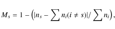
|
(5) |
where ns is the number density of the tracers within a cell (at the highest resolution level) and the sum refers to all the species of tracers. This formula generalizes the more simple case of mixing between two species (e.g. Ritchie & Thomas 2002).
The total mixing in each cell, M, is the volume average between all species,
![]() ,
where Ns is the number of families considered. The interpretation of this parameter is simple: for a cell where
,
where Ns is the number of families considered. The interpretation of this parameter is simple: for a cell where
![]() the different families are well mixed and we have
the different families are well mixed and we have
![]() ,
while
,
while
![]() implies no mixing within the cell.
implies no mixing within the cell.
Figure 15 shows the projected distributions of the mixing parameter ![]() at z=0
for the three clusters considered above together with projected maps of
gas pressure along the line of sight. We found that the differences in
the dynamical history of the three objects produce different spatial
distribution of mixing at z=0. H3 shows a uniform pattern of mixing, with
at z=0
for the three clusters considered above together with projected maps of
gas pressure along the line of sight. We found that the differences in
the dynamical history of the three objects produce different spatial
distribution of mixing at z=0. H3 shows a uniform pattern of mixing, with
![]() across the whole cluster core. On the other hand H5 presents the most patchy mixing map with a large plume of the size of
across the whole cluster core. On the other hand H5 presents the most patchy mixing map with a large plume of the size of ![]() Mpc in the direction of the major merger
and a maximum mixing of
Mpc in the direction of the major merger
and a maximum mixing of
![]() between the cores of merging clusters.
between the cores of merging clusters.
| Figure 10:
Phase distribution for four tracers runs, with decreasing sampling of
the underlying Eulerian grid: from left to right, N=106, N=105, N=5 |
|
| Open with DEXTER | |
![\begin{figure}
\par\includegraphics[width=17cm,clip]{images/13464f14.ps}
\vspace*{2mm}
\end{figure}](/articles/aa/full_html/2010/05/aa13464-09/img123.png)
|
Figure 11: Projected paths of three couples of tracers evolved from z=30to z=0 from an initial separation of 1 cell = 36 kpc, for run H7. Isocontours show the projected gas density at z=0. The side of the image is 3.8 Mpc. |
| Open with DEXTER | |
![\begin{figure}
\par\includegraphics[width=7.8cm,clip]{images/13464f15.ps}
\end{figure}](/articles/aa/full_html/2010/05/aa13464-09/img127.png)
|
Figure 12:
Time evolution of the pair tracers dispersion for N=106 tracers in run H7. Couples with three initial separations are considered:
|
| Open with DEXTER | |
In Fig. 16 we
compare the evolution of the gas entropy profiles for H1
and H5 (top panels) with that of the mixing profiles (bottom
panels). We found that efficient mixing is always confined in central
low entropy regions. The very regular evolution of mixing in H1
closely reflects the regular evolution of the gas entropy profile.
At the final epoch of observation, a flat mixing profile with
![]() was found within the entropy core at
was found within the entropy core at
![]() ,
and outside this core
,
and outside this core ![]() falls quickly to very low values. This is not surprising: in the
idealized ICM represented by these simulations, convective stability to
radial displacement is provided by the classic Schwarzschild
criterion,
falls quickly to very low values. This is not surprising: in the
idealized ICM represented by these simulations, convective stability to
radial displacement is provided by the classic Schwarzschild
criterion,
![]() (Schwarzschild 1959). A very flat entropy core is just marginally stable to radial perturbations, whereas
the steep rise of the entropy profile at
(Schwarzschild 1959). A very flat entropy core is just marginally stable to radial perturbations, whereas
the steep rise of the entropy profile at
![]() provides
a very stable configuration to radial perturbations. The situation is
more complex for the major merger system H5. The merger event at
provides
a very stable configuration to radial perturbations. The situation is
more complex for the major merger system H5. The merger event at
![]() affects the entropy profile and also drives a more extended pattern of
mixing. At the final epoch a peak of mixing is found at
affects the entropy profile and also drives a more extended pattern of
mixing. At the final epoch a peak of mixing is found at
![]() ,
and significant mixing is found even out of
,
and significant mixing is found even out of
![]() .
.
![\begin{figure}
\par\includegraphics[width=8cm,clip]{images/13464f16.ps}\hspace*{0.5cm}
\includegraphics[width=7.9cm,clip]{images/13464f17.ps}
\end{figure}](/articles/aa/full_html/2010/05/aa13464-09/img135.png)
|
Figure 13:
Left: time evolution of the pair of tracers dispersion for N=2 |
| Open with DEXTER | |
![\begin{figure}
\par\mbox{\includegraphics[width=4.2cm,clip]{images/13464f18.ps}\...
...464f28.ps}\includegraphics[width=4.2cm,clip]{images/13464f29.ps} }\end{figure}](/articles/aa/full_html/2010/05/aa13464-09/img138.png)
|
Figure 14:
Evolution of projected positions of tracer families for run H3 ( top panels), H1 ( central panels) and H5 ( lower panels).
Every color refers to a different shell of origin. Overlaid are
the contours of the projected gas density (the first contour is
for
|
| Open with DEXTER | |
This large mixing pattern in extended merger systems confirms previous works that analyzed idealized 2-body encounters with the SPH techniques (e.g. Ritchie & Thomas 2002; Ascasibar & Markevitch 2006), and thus our exploratory study extends their results to fully cosmological Eulerian simulations. In addition, as shown by Mitchell et al. (2009), major mergers in Eulerian AMR codes are more efficient in mixing the ICM compared to mergers in SPH codes, since in SPH mixing during the central stages of the merger is significantly prevented by the suppression of instabilities by the artificial particles viscosity; our findings seem to support the presence of large eddies that provide efficient mixing during the central stages of cluster mergers. It is important to compare results for the evolution of mixing obtained through our refinement strategy (Sect. 2.2) with those obtained with a standard mesh refinement strategy. For this purpose we re-simulated cluster H1, allowing only for mesh refinement according to the gas/over-density criterion and applied the same initial setup of spherical shells of tracers to measure the evolution of mixing at all times (Fig. 17). Even if the overall behavior is similar, the refinement criterion using velocity jumps and gas/DM over-density produces a larger mixing especially at large radii, and the progressive accretion of this gas also induces large mixing in the innermost cluster regions at later redshifts. This clearly shows that the artificial suppression of chaotic motions due to coarse numerical resolution may reduce in a sizable way the mixing in the simulated ICM, even within the virial volume of clusters.
![\begin{figure}
\par\includegraphics[width=8.5cm,clip]{images/13464f30.ps}\par\in...
...64f31.ps}\par\includegraphics[width=8.5cm,clip]{images/13464f32.ps}
\end{figure}](/articles/aa/full_html/2010/05/aa13464-09/img139.png)
|
Figure 15: Map of projected gas pressure ( left panels) and of projected tracers mixing ( right) panels, for run H3 ( top), H1 ( center) and H5 ( bottom) at z=0. The side of the images and the LOS are 5 Mpc; the mixing maps are produced by considering only cells containing more than one tracer. |
| Open with DEXTER | |
![\begin{figure}
\par\includegraphics[width=4.2cm,clip]{images/13464f36.ps}\hspace...
...hspace*{3mm}
\includegraphics[width=4.2cm,clip]{images/13464f39.ps}
\end{figure}](/articles/aa/full_html/2010/05/aa13464-09/img140.png)
|
Figure 16: Evolution of gas entropy profile ( top panels) and of mean mixing ( bottom panels) for H1 ( left) and H5 ( right). |
| Open with DEXTER | |
![\begin{figure}
\par\includegraphics[width=8cm,clip]{images/13464f40.ps}\vspace{-4.5mm}
\end{figure}](/articles/aa/full_html/2010/05/aa13464-09/img141.png)
|
Figure 17: Evolution of mean mixing profile for cluster H1 at three redshifts, for the standard mesh refinement strategy ( dashed lines) and for our implemented mesh refinement strategy ( solid lines). |
| Open with DEXTER | |
4.3 Application to the metal mixing in the ICM
X-ray observations proved that the ICM hosts ![]() per cent of heavy elements in mass, corresponding to a mean metallicity
per cent of heavy elements in mass, corresponding to a mean metallicity
![]() ,
where
,
where ![]() is the solar metallicity (e.g. Werner et al. 2008,
for a up-to-date review). The distribution of metals in galaxy
clusters is characterized by profiles that are peaked toward the core
of cooling flow clusters and rather flat in all the others (Vikhlinin
et al. 2005; Pratt et al. 2007). Two dimensional metallicity maps from nearby clusters provided evidence for
complex and non symmetric distributions of heavy elements (e.g. Sanders & Fabian 2006; Finoguenov et al. 2006).
Furthermore, recent observations shed some light on the significant
evolution with decreasing redshift of the cluster metallicity (Balestra
et al. 2007; Maughan et al. 2007).
is the solar metallicity (e.g. Werner et al. 2008,
for a up-to-date review). The distribution of metals in galaxy
clusters is characterized by profiles that are peaked toward the core
of cooling flow clusters and rather flat in all the others (Vikhlinin
et al. 2005; Pratt et al. 2007). Two dimensional metallicity maps from nearby clusters provided evidence for
complex and non symmetric distributions of heavy elements (e.g. Sanders & Fabian 2006; Finoguenov et al. 2006).
Furthermore, recent observations shed some light on the significant
evolution with decreasing redshift of the cluster metallicity (Balestra
et al. 2007; Maughan et al. 2007).
From the theoretical point of view, several processes can contribute to the observed patterns and evolution of metals in the ICM: galactic winds, ram pressure stripping, galaxy-galaxy interactions, intra-cluster supernovae, intra-cluster stellar populations etc. (e.g. Schindler & Diaferio 2008, and references therein). Dealing with all these multi-physics and multi-scale processes is a challenging task for any cosmological simulation. As a consequence, although the overall scenario of metals evolution can be reproduced by simulations with an acceptable agreement with observations (e.g. Cora 2006; Kapferer et al. 2007; Tornatore et al. 2007; Wiersma et al. 2009), the details of the process are still largely uncertain.
Although our simulations do not account for any treatment of chemical elements production and evolution, our tracer method can provide new hints about the ways injected metals are spread and mixed in the ICM during cluster evolution.
We present here a simple set of exploratory studies, where
initial injection profiles of metal tracers are assumed to reproduce
the metal release from galactic winds, and where the advection of metal
tracers is followed as a function of the evolution of the underlying
gas distribution. The DM mass resolution in our runs is high
enough to detect single galaxy-like structures in the DM distribution by means of the same halo-finder algorithm mentioned in Sect. 4.2. Therefore below we will use the term galaxy for massive DM clumps with
![]() DM particles. We explore three (idealized) scenarios describing the initial
injection of ``metal tracers'': a) a single injection at z=1 from the central cluster galaxy; b) ten injections which are spaced in time (in the range 1<z<0) from the central cluster galaxy; c) ten injections as in case ``b'' (in the range 1<z<0) from the ten most massive galaxies within the AMR volume.
DM particles. We explore three (idealized) scenarios describing the initial
injection of ``metal tracers'': a) a single injection at z=1 from the central cluster galaxy; b) ten injections which are spaced in time (in the range 1<z<0) from the central cluster galaxy; c) ten injections as in case ``b'' (in the range 1<z<0) from the ten most massive galaxies within the AMR volume.
Following Rebusco et al. (2006), we modeled the profile of injected metals from a galaxy with a ![]() -profile
-profile

|
(6) |
where a0 is the solar abundance, ra is the scale radius for each galaxy, and
![\begin{figure}
\par\mbox{\includegraphics[width=4.3cm,clip]{images/13464f41.ps}\...
...464f43.ps}\includegraphics[width=4.3cm,clip]{images/13464f44.ps} }\end{figure}](/articles/aa/full_html/2010/05/aa13464-09/img152.png)
|
Figure 18:
Time evolution of the projected positions for metal tracers
injected at z=1 from a single cD galaxy in the center of H1. Gas density contours are generated as in Fig. 14, the side of the images is
|
| Open with DEXTER | |
Our choice of parameters was just a trial, designed to fall within the range of the parameters for galaxies studied in Rebusco et al. (2006). With this simple setup, we explored the effects played by spatial transport on the mixing of metals deposited in the evolving ICM.
In Fig. 18 we show the evolution of the projected positions of
![]()
![]() 104 metal tracers in the cluster H1 for model ``a''.
104 metal tracers in the cluster H1 for model ``a''.
Even if the dynamical history of this cluster at z=0 is fairly regular, the amount of mergers and
accretions of matter experienced at ![]() is enough to spread the metals out to
is enough to spread the metals out to
![]()
![]() .
.
The evolution of the number density profile of metal tracers from a single injection at z=1 (model ``a'') is shown in the left panel in Fig. 19 for the same cluster. This injection scenario produces a very flat distribution of metals at
![]() .
Even if the qualitative behavior is similar to that reported in Rebusco et al. (2005), we notice that in our case the distance where metal pollution is efficient in the ICM is larger, which is
consistent with the larger transport pattern presented in Sect. 4.2.
.
Even if the qualitative behavior is similar to that reported in Rebusco et al. (2005), we notice that in our case the distance where metal pollution is efficient in the ICM is larger, which is
consistent with the larger transport pattern presented in Sect. 4.2.
The result of ten injection epochs (one every
![]() )
from the central galaxy (model ``b'') is shown in the central panel in Fig. 19. This obviously increases by
)
from the central galaxy (model ``b'') is shown in the central panel in Fig. 19. This obviously increases by ![]() the final metal content in the innermost cluster region and is found to
produce a monotonically decreasing tracer distribution at
all radii.
the final metal content in the innermost cluster region and is found to
produce a monotonically decreasing tracer distribution at
all radii.
![\begin{figure}
\par\includegraphics[width=5.5cm,clip]{images/13464f45.ps}\hspace...
...pace*{1.5mm}
\includegraphics[width=5.5cm,clip]{images/13464f47.ps}
\end{figure}](/articles/aa/full_html/2010/05/aa13464-09/img159.png)
|
Figure 19: Evolution of the number profile of metal tracers for cluster H1, for the 3 injection recipes introduced in Sect. 4.3: single injection at z=1 from the central cD galaxy ( left), several injections from the central cD galaxy ( center) and several injections from 10 galaxies ( right). The contribution from each galaxy in the ``c'' model has been normalized as explained in Sect. 4.3. |
| Open with DEXTER | |
A case of more astrophysical relevance is perhaps our model ``c'', which assumes multiple injections from the ten most massive galaxies in the AMR region (see right panel in Fig. 19). The corresponding spatial evolution of metal tracers in cluster H1 with overlaid gas density contours, is shown in Fig. 20. In this case the metal distribution is quite regular at all redshifts compared to the case of injection from the central cluster galaxy only.
The role played by mergers in the disruption of cool cores is still an object of debate (e.g. Santos et al. 2009, and references therein), although observations support the destruction of cool-cores by cluster mergers (Allen et al. 2001; Sanderson et al. 2006; Rossetti & Molendi 2010). Indeed, observations suggest a dichotomy between the metallicity profiles in the cool-core and non-cool core clusters (e.g. De Grandi et al. 2004). Our simulations neglect any treatment of cooling and of energy feedback mechanisms from central AGN, and consequently we cannot address this in a self-consistent way. We can speculate though that the most relaxed clusters in our sample are similar to cool core clusters, while clusters with mergers are more similar to non-cool core clusters.
![\begin{figure}
\par\mbox{\includegraphics[width=4.3cm,clip]{images/13464f48.ps}\...
...cludegraphics[width=4.3cm,clip]{images/13464f51.ps} }
\vspace{-3mm}
\end{figure}](/articles/aa/full_html/2010/05/aa13464-09/img161.png)
|
Figure 20:
Time evolution of the projected positions for metal tracers
injected every
|
| Open with DEXTER | |
![\begin{figure}
\par\includegraphics[width=8cm,clip]{images/13464f52.ps}
\end{figure}](/articles/aa/full_html/2010/05/aa13464-09/img162.png)
|
Figure 21: Mean metallicity profile for the relaxed clusters H1 and H3 (triangles) and for the perturbed clusters H5 and H6 (crosses) at z=0.1. |
| Open with DEXTER | |
We calculated the metallicity profiles for four clusters in our sample
(two with a fairly relaxed dynamical evolution and two with a
major merger in the range
![]() )
to investigate the effect of cluster dynamics on the shape of
metallicity profiles. The total iron mass in the ICM is normalized so
that the metallicity at the position of the central galaxy in the
cluster was Z=1; the gas mass was directly taken from the cells in the simulation. In Fig. 21 we show the profiles of the four clusters at
)
to investigate the effect of cluster dynamics on the shape of
metallicity profiles. The total iron mass in the ICM is normalized so
that the metallicity at the position of the central galaxy in the
cluster was Z=1; the gas mass was directly taken from the cells in the simulation. In Fig. 21 we show the profiles of the four clusters at
![]() .
The profiles are computed for spherical shells of a width of
36 kpc and they were centered on the peak of the X-ray bolometric
cluster emission; the contribute of freshly (un-evolved) metal tracers
from the central cluster galaxy at the redshift of observation was
removed in post-processing.
.
The profiles are computed for spherical shells of a width of
36 kpc and they were centered on the peak of the X-ray bolometric
cluster emission; the contribute of freshly (un-evolved) metal tracers
from the central cluster galaxy at the redshift of observation was
removed in post-processing.
We found a remarkable trend: ``relaxed'' clusters showed a very peaked metallicity profile, while ``merger'' clusters showed a more complex behavior with flat profiles up to the outer regions. Since the injection of metal tracers in all runs was done in the same way and with the same duty cycles and no physical mechanism other than hierarchical clustering was at work here, this test suggests that very different metallicity profiles in the ICM may result from the effect of different matter accretion histories.
Future works accounting for a realistic chemical enrichment model and cooling/feedback processes may produce quantitative and self-consistent predictions, yet our results qualitatively suggest that the observed dichotomy of metallicity profiles might be simply explained in terms of different cluster dynamics; tracers offer a valuable method to investigate this important issue.
![\begin{figure}
\par\includegraphics[width=4cm,clip]{images/13464f53.ps}\hspace*{...
...}\hspace*{3mm}
\includegraphics[width=4cm,clip]{images/13464f56.ps}
\end{figure}](/articles/aa/full_html/2010/05/aa13464-09/img163.png)
|
Figure 22: Simulated iron line profile for clusters H1, H3, H4 and H5. The red lines show the line emissivity simulated assuming the tracer metallicity, the black lines are for a constant metallicty and the blue lines are for an average metallicity which scales with radius. |
| Open with DEXTER | |
4.4 Iron line profile
Turbulent gas motions can lead to a Doppler shift broadening of X-ray
emitting metal lines, in excess to their intrinsic width.
Measuring the broadening of metal lines in the future will likely
provide the most direct evidence of subsonic turbulent motions in the
ICM![]() In a number of works (Sunyaev et al. 2003; Inogamov & Sunyaev 2003; Dolag et al. 2005)
it was proved that if turbulent motions are at the level of what
is produced in cosmological numerical simulations, the shape of
the Fe XXIII line would be enough modified to allow studies
of turbulence in the ICM. Here we extend these works by taking
into account the 3D metallicity distribution that comes out in our
simulations adopting the ``c'' model as fiducial injection model
for metal tracers.
In a number of works (Sunyaev et al. 2003; Inogamov & Sunyaev 2003; Dolag et al. 2005)
it was proved that if turbulent motions are at the level of what
is produced in cosmological numerical simulations, the shape of
the Fe XXIII line would be enough modified to allow studies
of turbulence in the ICM. Here we extend these works by taking
into account the 3D metallicity distribution that comes out in our
simulations adopting the ``c'' model as fiducial injection model
for metal tracers.
We thus estimated the emission along the line of sight of the
6.702 keV iron line with columns through the center of the
four galaxy clusters in our sample. For every tracer we assumed a
line emissivity proportional to the second power of its metal content
(which was derived as in Sect. 4.3),
and for simplicity we neglected any dependence on the gas temperature.
The effect of thermal broadening and the blending with other iron lines
is also neglected. As a control check, we also computed two
additional iron emissivities directly from the cells of the
simulations: in the first case we simply assumed a fixed
metallicity for all cells, and in the second case we assumed a uniform
metallicity radial profile in the form of
![]() (e.g. Vikhlinin et al. 2005). In all cases, the velocity of the center of mass of every cluster has been removed.
(e.g. Vikhlinin et al. 2005). In all cases, the velocity of the center of mass of every cluster has been removed.
Figure 22 shows the simulated iron line profile, for clusters H1, H3, H4 and H5 at z=0. For every cluster the signal was extracted along columns with a section of
![]() and an energy resolution of
and an energy resolution of
![]() was assumed. All emissions were normalized to have the same total luminosity = 1 within the column.
was assumed. All emissions were normalized to have the same total luminosity = 1 within the column.
For clusters without a major merger, the centroid of the iron line and the general shape of the line from the tracers agreed reasonably with those from the cells. In the case of the major merger system (H5) the centroids and the shapes of the lines were quite different. Consistently with what was found in the previous sections, this is because mergers create complex and patchy distributions of metal tracers, which cannot be fully described by a simple radial profile. This is further highlighted in Fig. 23, which is obtained at the epoch of the major merger in H5.
We conclude that the realistic modeling of the iron line broadening requires an appropriate modeling of the distribution of metals in the cluster volume.
Tracers also allow for the decomposition of the convoluted iron
line profile in the contributions from the different generations of
metal tracers. Figure 24
shows the comparison of the emissivity profile for cluster H1, H3
and H5 (in this case the section of the column is set to
![]() to also highlight the contribution from tracers distributed at
larger distances from the cluster center) and the relative
contributions from different generations of tracers. The case of the
the major merger system highlights that the signal from the total iron
line is the convolution of very different emissions coming from
different generations of metal tracers and that the earlier generations
are responsible for much broader and asymmetric components compared to
the latest generations that were injected after the major merger.
to also highlight the contribution from tracers distributed at
larger distances from the cluster center) and the relative
contributions from different generations of tracers. The case of the
the major merger system highlights that the signal from the total iron
line is the convolution of very different emissions coming from
different generations of metal tracers and that the earlier generations
are responsible for much broader and asymmetric components compared to
the latest generations that were injected after the major merger.
![\begin{figure}
\par\includegraphics[width=8cm,clip]{images/13464f57.ps}
\end{figure}](/articles/aa/full_html/2010/05/aa13464-09/img168.png)
|
Figure 23: Simulated iron line profile for cluster H5 at z=0.5. The meaning of lines is the same of Fig. 22. |
| Open with DEXTER | |
![\begin{figure}
\par\includegraphics[width=5.5cm,clip]{images/13464f58.ps}\hspace...
...includegraphics[width=5.5cm,clip]{images/13464f60.ps}
\vspace*{5mm}
\end{figure}](/articles/aa/full_html/2010/05/aa13464-09/img169.png)
|
Figure 24: Simulated iron line profile for clusters H1, H3 and H5 at z=0. The black lines show the total line emissivity, while the colored lines show the contribution for a sub-sample of tracer generations at different epochs. |
| Open with DEXTER | |
5 Conclusions
In this work we studied the mixing properties of the ICM in simulated
galaxy clusters, using tracer particles that are advected by the gas
flow during the evolution of cosmic structures.
This approach allowed us to obtain valuable information on the
Lagrangian properties of the ICM, and allowed progress in our
understanding of the transport processes in Eulerian simulations of
galaxy clusters. Seven galaxy clusters with total masses in the range
![]()
![]()
![]() and different dynamical states were simulated with an updated version
of the ENZO code (Norman et al. 2007), where an additional refinement criterion was designed to reach good spatial accuracy at shock waves up to
and different dynamical states were simulated with an updated version
of the ENZO code (Norman et al. 2007), where an additional refinement criterion was designed to reach good spatial accuracy at shock waves up to
![]() from the center of galaxy clusters (Vazza et al. 2009a,b).
In a post-processing, we injected and followed passive
tracers, and tracked their spatial evolution with high time resolution.
Numerical tests were presented and discussed to find the optimal
strategies to inject tracers, update their positions
in time and sample the galaxy cluster volume (Sect. 3). We then applied this tracer technique to some interesting problems concerning the mixing of the ICM.
from the center of galaxy clusters (Vazza et al. 2009a,b).
In a post-processing, we injected and followed passive
tracers, and tracked their spatial evolution with high time resolution.
Numerical tests were presented and discussed to find the optimal
strategies to inject tracers, update their positions
in time and sample the galaxy cluster volume (Sect. 3). We then applied this tracer technique to some interesting problems concerning the mixing of the ICM.
First, we showed that the pair dispersion statistics has a well
constrained behavior in time: for most of the cosmic time the
separation between close couples of tracers shows a very regular
evolution in all clusters, consistently with the basic
![]() scaling expected for a simple turbulent model (Sect. 4.1).
This finding is well consistent with the independent measurement of
3D velocity power spectrum for the same clusters, and confirms
that a sizable amount of complex subsonic motions correlated on cluster
scales account for 10-30 per cent of the thermal energy
inside
scaling expected for a simple turbulent model (Sect. 4.1).
This finding is well consistent with the independent measurement of
3D velocity power spectrum for the same clusters, and confirms
that a sizable amount of complex subsonic motions correlated on cluster
scales account for 10-30 per cent of the thermal energy
inside
![]() of our simulated clusters.
of our simulated clusters.
Second, we quantified the degree of radial mixing of the ICM by
following the evolution of tracers injected in regular shells within
the cluster volume at
![]() .
The radial mixing morphology was found to be strongly dependent on the
dynamical history of every cluster. Large plumes (with the size
of
.
The radial mixing morphology was found to be strongly dependent on the
dynamical history of every cluster. Large plumes (with the size
of
![]() )
where gas matter is efficiently mixed were found for a major merger
cluster. On the other hand more regular and concentrated mixing
profiles were measured for more relaxed clusters.
)
where gas matter is efficiently mixed were found for a major merger
cluster. On the other hand more regular and concentrated mixing
profiles were measured for more relaxed clusters.
Third, we assumed a simple model of metal injection from galaxies identified in the simulations around the clusters and studied the metal enrichment of the ICM by tracking the advection of ``metal'' tracers (tracers with a different iron content as a function of their galaxy of origin) deposited in the cluster volume. In this case also, the dynamical state of galaxy clusters and its matter accretion history were found to affect the final distribution of metal tracers at evolved epochs. In particular, the simulated clusters showed a hint of dichotomy in metallicity distributions between clusters experiencing only minor mergers and clusters with major mergers, with the latter showing a broader distribution of metals.
Finally, we simulated the emissivity of the Fe XXIII line from the center of our clusters, using the 3D distribution of metals produced through our metal tracer injection (model ``c''). We reported significant departures from the simplified assumption of a constant or a radially symmetric metallicity profile, particularly for merger systems. This stresses the importance of studying in detail the connection between the metal enrichment history and the matter accretion history of the ICM.
In conclusions, we believe that the coupling of high resolution Eulerian numerical simulations and a tracer technique represents a very powerful tool to study crucial open problems concerning the mixing properties of the diffuse gas in galaxy clusters, and the injection and the advection of cosmic rays particles in galaxy clusters, which will be subject of future works.
We thank the anonymous referee, whose suggestions helped us to improve the presentation of this paper. The authors thank R. Brunino for valuable support at CINECA Supercomputing Center, M. Nanni, F. Tinarelli and M. Tugnoli for valuable technical support at the Radio Astronomy Institute (Bologna), and G. Tormen for useful discussions. We acknowledge partial support through grant ASI-INAF I/088/06/0 and PRIN INAF 2007/2008, and the use of computational resources under the CINECA-INAF 2008-2010 agreement.
References
- Agertz, O., Moore, B., Stadel, J., et al. 2007, MNRAS, 380, 963 [NASA ADS] [CrossRef] [Google Scholar]
- Aharonian, F., Akhperjanian, A. G., de Almeida, U. B., et al. 2009, ApJ, 691, 175 [NASA ADS] [CrossRef] [Google Scholar]
- Allen, S. W., Schmidt, R. W., & Fabian, A. C. 2001, MNRAS, 328, L37 [NASA ADS] [CrossRef] [Google Scholar]
- Arzner, K., Knaepen, B., Carati, D., Denewet, N., & Vlahos, L. 2006, ApJ, 637, 322 [NASA ADS] [CrossRef] [Google Scholar]
- Ascasibar, Y., & Markevitch, M. 2006, ApJ, 650, 102 [NASA ADS] [CrossRef] [Google Scholar]
- Balestra, I., Tozzi, P., Ettori, S., et al. 2007, A&A, 462, 429 [NASA ADS] [CrossRef] [EDP Sciences] [Google Scholar]
- Bec, J., Biferale, L., Cencini, M., Lanotte, A. S., & Toschi, F. 2006, unpublished [arXiv:nlin/0604059] [Google Scholar]
- Bec, J., Biferale, L., Lanotte, A. S., Scagliarini, A., & Toschi, F. 2010, J. Fluid Mech., 646, 527 [NASA ADS] [CrossRef] [Google Scholar]
- Berger, M. J., & Oliger, J. 1984, J. Comput. Phys., 53, 484 [NASA ADS] [CrossRef] [MathSciNet] [Google Scholar]
- Berger, M. J., & Colella, P. 1989, JCoPh, 82, 64 [Google Scholar]
- Biferale, L., Boffetta, G., Celani, A., et al. 2004, Phys. Rev. Lett., 93, 064502 [NASA ADS] [CrossRef] [PubMed] [Google Scholar]
- Bonafede, A., Feretti, L., Murgia, M., et al. 2010, A&A, 513, A30 [NASA ADS] [CrossRef] [EDP Sciences] [Google Scholar]
- Borgani, S., Fabjan, D., Tornatore, L., et al. 2008, Space Sci. Rev., 134, 379 [NASA ADS] [CrossRef] [Google Scholar]
- Bosse, T., Kleiser, L., & Meiburg, E. 2006, Phys. Fluids, 18, 027102 [NASA ADS] [CrossRef] [Google Scholar]
- Brüggen, M., & Kaiser, C. R. 2002, Nature, 418, 301 [NASA ADS] [CrossRef] [PubMed] [Google Scholar]
- Brunetti, G., & Lazarian, A. 2007, MNRAS, 378, 245 [NASA ADS] [CrossRef] [Google Scholar]
- Brunetti, G., Venturi, T., Dallacasa, D., et al. 2007, ApJ, 670, L5 [NASA ADS] [CrossRef] [Google Scholar]
- Brunetti, G., Giacintucci, S., Cassano, R., et al. 2008, Nature, 455, 944 [NASA ADS] [CrossRef] [Google Scholar]
- Bryan, G. L., & Norman, M. L. 1997, ASPC, 123, 363 [NASA ADS] [Google Scholar]
- Bryan, G. L., Norman, M. L., Stone, J. M., Cen, R., & Ostriker, J. P. 1995, CoPhC, 89, 149 [Google Scholar]
- Calzavarini, E., Cencini, M., Lohse, D., & Toschi, F. 2008, Phys. Rev. Lett., 101, 084504 [NASA ADS] [CrossRef] [PubMed] [Google Scholar]
- Churazov, E., Forman, W., Jones, C., & Böhringer, H. 2003, ApJ, 590, 225 [NASA ADS] [CrossRef] [Google Scholar]
- Cora, S. A. 2006, MNRAS, 368, 1540 [Google Scholar]
- Couchman, H. M. P., Thomas, P. A., & Pearce, F. R. 1995, ApJ, 452, 797 [NASA ADS] [CrossRef] [Google Scholar]
- De Grandi, S., Ettori, S., Longhetti, M., & Molendi, S. 2004, A&A, 419, 7 [NASA ADS] [CrossRef] [EDP Sciences] [Google Scholar]
- Dolag, K., Vazza, F., Brunetti, G., & Tormen, G. 2005, MNRAS, 364, 753 [NASA ADS] [CrossRef] [Google Scholar]
- Elhmaidi, D., Provenzale, A., & Babiano, A. 1993, J. Fluid Mech., 257, 533 [NASA ADS] [CrossRef] [Google Scholar]
- Federrath, C., Glover, S. C. O., Klessen, R. S., & Schmidt, W. 2008, Physica Scripta Volume T, 132, 014025 [NASA ADS] [CrossRef] [Google Scholar]
- Ferrari, C., Govoni, F., Schindler, S., Bykov, A., & Rephaeli, Y. 2008, SSR [Google Scholar]
- Finoguenov, A., Henriksen, M. J., Miniati, F., Briel, U. G., & Jones, C. 2006, ApJ, 643, 790 [NASA ADS] [CrossRef] [Google Scholar]
- Fryxell, B., Olson, K., Ricker, P., et al. 2000, ApJS, 131, 273 [NASA ADS] [CrossRef] [Google Scholar]
- Gheller, C., Pantano, O., & Moscardini, L. 1998, MNRAS, 296, 85 [NASA ADS] [CrossRef] [Google Scholar]
- Godunov, S. K. 1959, Mat. Sbornik, 47, 271 [Google Scholar]
- Henry, J. P., Finoguenov, A., & Briel, U. G. 2004, ApJ, 615, 181 [NASA ADS] [CrossRef] [Google Scholar]
- Hockney, R. W., & Eastwood, J. W. 1981, Computer Simulation Using Particles (New York: McGraw-Hill) [Google Scholar]
- Iapichino, L., & Niemeyer, J. C. 2008, MNRAS, 388, 1089 [NASA ADS] [CrossRef] [Google Scholar]
- Inogamov, N. A., & Sunyaev, R. A. 2003, Astron. Lett., 29, 791 [NASA ADS] [CrossRef] [Google Scholar]
- Kapferer, W., Kronberger, T., Weratschnig, J., & Schindler, S. 2007, A&A, 472, 757 [NASA ADS] [CrossRef] [EDP Sciences] [Google Scholar]
- Kitsionas, S., Federrath, C., Klessen, R. S., et al. 2009, A&A, 508, 541 [NASA ADS] [CrossRef] [EDP Sciences] [Google Scholar]
- Kravtsov, A. V., Klypin, A. A., & Khokhlov, A. M. 1997, ApJS, 111, 73 [NASA ADS] [CrossRef] [Google Scholar]
- Kuchar, P., & Ensslin, T. A. 2009, A&A, submitted [arXiv:0912.3930] [Google Scholar]
- Lau, E. T., Nagai, D., & Kravtsov, A. V. 2010, ApJ, 708, 1419 [NASA ADS] [CrossRef] [Google Scholar]
- Maier, A., Iapichino, L., Schmidt, W., & Niemeyer, J. C. 2009, ApJ, 707, 40 [NASA ADS] [CrossRef] [Google Scholar]
- Markevitch, M., & Vikhlinin, A. 2007, Phys. Rep., 443, 1 [NASA ADS] [CrossRef] [EDP Sciences] [Google Scholar]
- Maughan, B. J., Jones, C., Jones, L. R., & Van Speybroeck, L. 2007, ApJ, 659, 1125 [NASA ADS] [CrossRef] [Google Scholar]
- Maxey, M. R., & Riley, J. J. 1983, Phys. Fluids, 26, 883 [NASA ADS] [CrossRef] [Google Scholar]
- Mitchell, N. L., McCarthy, I. G., Bower, R. G., Theuns, T., & Crain, R. A. 2009, MNRAS, 395, 180 [NASA ADS] [CrossRef] [Google Scholar]
- Murgia, M., Govoni, F., Feretti, L., et al. 2004, A&A, 424, 429 [NASA ADS] [CrossRef] [EDP Sciences] [Google Scholar]
- Nagai, D., Kravtsov, A. V., & Vikhlinin, A. 2007, ApJ, 668, 1 [NASA ADS] [CrossRef] [Google Scholar]
- Norman, M. L., & Bryan, G. L. 1999, The Radio Galaxy Messier 87, 530, 106 [NASA ADS] [CrossRef] [Google Scholar]
- Norman, M. L., Bryan, G. L., Harkness, R., et al. 2007, in Petascale Computing: Algorithms and Applications, ed. D. Bader (CRC Press LLC) [arXiv:0705.1556] [Google Scholar]
- Omma, H., Binney, J., Bryan, G., & Slyz, A. 2004, MNRAS, 348, 1105 [NASA ADS] [CrossRef] [Google Scholar]
- O'Shea, B. W., Nagamine, K., Springel, V., Hernquist, L., & Norman, M. L. 2005, ApJS, 160, 1 [NASA ADS] [CrossRef] [Google Scholar]
- Parrish, I. J., & Stone, J. M. 2005, ApJ, 633, 334 [NASA ADS] [CrossRef] [Google Scholar]
- Pfrommer, C., Springel, V., Enßlin, T. A., & Jubelgas, M. 2006, MNRAS, 367, 113 [NASA ADS] [CrossRef] [Google Scholar]
- Porter, D. H., & Woodward, P. R. 1994, ApJS, 93, 309 [NASA ADS] [CrossRef] [Google Scholar]
- Pratt, G. W., Böhringer, H., Croston, J. H., et al. 2007, A&A, 461, 71 [NASA ADS] [CrossRef] [EDP Sciences] [Google Scholar]
- Quataert, E. 2008, ApJ, 673, 758 [NASA ADS] [CrossRef] [Google Scholar]
- Rebusco, P., Churazov, E., Böhringer, H., & Forman, W. 2005, MNRAS, 359, 1041 [NASA ADS] [CrossRef] [Google Scholar]
- Rebusco, P., Churazov, E., Böhringer, H., & Forman, W. 2006, MNRAS, 372, 1840 [Google Scholar]
- Reimer, O. 2004, JKAS, 37, 307 [NASA ADS] [Google Scholar]
- Richardson, L. F. 1926, Proc. Roy. Soc. A, 110, 709 [Google Scholar]
- Ritchie, B. W., & Thomas, P. A. 2002, MNRAS, 329, 675 [NASA ADS] [CrossRef] [Google Scholar]
- Robertson, B. E., Kravtsov, A. V., Gnedin, N. Y., Abel, T., & Rudd, D. H. 2010, MNRAS, 401, 2463 [NASA ADS] [CrossRef] [Google Scholar]
- Rossetti, M., & Molendi, S. 2010, A&A, 510, A83 [Google Scholar]
- Ruszkowski, M., & Oh, S. P. 2009, ApJ, submintted [arXiv:0911.5198] [Google Scholar]
- Ryu, D., Ostriker, J. P., Kang, H., & Cen, R. 1993, ApJ, 414, 1 [NASA ADS] [CrossRef] [Google Scholar]
- Ryu, D., Kang, H., Hallman, E., & Jones, T. W. 2003, ApJ, 593, 599 [NASA ADS] [CrossRef] [Google Scholar]
- Sanders, J. S., & Fabian, A. C. 2006, MNRAS, 371, 1483 [NASA ADS] [CrossRef] [Google Scholar]
- Sanders, J. S., Fabian, A. C., Smith, R. K., & Peterson, J. R. 2009, MNRAS, L359 [Google Scholar]
- Sanderson, A. J. R., Ponman, T. J., & O'Sullivan, E. 2006, MNRAS, 372, 1496 [NASA ADS] [CrossRef] [Google Scholar]
- Santos, J. S., Rosati, P., Gobat, R., et al. 2009, A&A, 501, 49 [NASA ADS] [CrossRef] [EDP Sciences] [Google Scholar]
- Schindler, S., & Diaferio, A. 2008, Space Sci. Rev., 134, 363 [NASA ADS] [CrossRef] [Google Scholar]
- Schuecker, P., Finoguenov, A., Miniati, F., Böhringer, H., & Briel, U. G. 2004, A&A, 426, 387 [NASA ADS] [CrossRef] [EDP Sciences] [Google Scholar]
- Schumacher, J., & Eckhardt, B. 2002, Phys. Rev. E, 66, 017303 [NASA ADS] [CrossRef] [Google Scholar]
- Schwarzschild, M. 1959, ApJ, 130, 345 [NASA ADS] [CrossRef] [Google Scholar]
- Sharma, P., Chandran, B. D. G., Quataert, E., & Parrish, I. J. 2009, in The Monster's Fiery Breath, ed. S. Heinz, & E. Wilcots, AIP Conf. Ser. [arXiv:0909.0270] [Google Scholar]
- Shtykovskiy, P., & Gilfanov, M. 2010, MNRAS, 401, 1360 [NASA ADS] [CrossRef] [Google Scholar]
- Springel, V. 2005, MNRAS, 364, 1105 [NASA ADS] [CrossRef] [Google Scholar]
- Springel, V. 2009, MNRAS, 1655 [Google Scholar]
- Subramanian, K., Shukurov, A., & Haugen, N. E. L. 2006, MNRAS, 366, 1437 [NASA ADS] [CrossRef] [Google Scholar]
- Sunyaev, R. A., Norman, M. L., & Bryan, G. L. 2003, AstL, 29, 783 [Google Scholar]
- Tasker, E. J., Brunino, R., Mitchell, N. L., et al. 2008, MNRAS, 390, 1267 [NASA ADS] [CrossRef] [Google Scholar]
- Teyssier, R. 2002, A&A, 385, 337 [NASA ADS] [CrossRef] [EDP Sciences] [Google Scholar]
- The MAGIC Collaboration: Aleksic, J., Pfrommer, C., Pinzke, A., et al. 2010, ApJ, 710, 634 [NASA ADS] [CrossRef] [Google Scholar]
- Tornatore, L., Borgani, S., Dolag, K., & Matteucci, F. 2007, MNRAS, 382, 1050 [NASA ADS] [CrossRef] [Google Scholar]
- Toschi, F., & Bodenschatz, E. 2009, Annu. Rev. Fluid Mech., 41, 375 [Google Scholar]
- Vacca, V., Murgia, M., Govoni, F., et al. 2010, A&A, in press [arXiv:1001.1058] [Google Scholar]
- Vazza, F., Tormen, G., Cassano, R., Brunetti, G., & Dolag, K. 2006, MNRAS, 369, L14 [NASA ADS] [Google Scholar]
- Vazza, F., Brunetti, G., & Gheller, C. 2009a, MNRAS, 395, 1333 [NASA ADS] [CrossRef] [Google Scholar]
- Vazza, F., Brunetti, G., Kritsuk, A., et al. 2009b, A&A, 504, 33 [NASA ADS] [CrossRef] [EDP Sciences] [Google Scholar]
- Vikhlinin, A., Markevitch, M., Murray, S. S., et al. 2005, ApJ, 628, 655 [NASA ADS] [CrossRef] [Google Scholar]
- Vogt, C., & Enßlin, T. A. 2005, A&A, 434, 67 [NASA ADS] [CrossRef] [EDP Sciences] [Google Scholar]
- Wadsley, J. W., Veeravalli, G., & Couchman, H. M. P. 2008, MNRAS, 387, 427 [NASA ADS] [CrossRef] [Google Scholar]
- Werner, N., Durret, F., Ohashi, T., Schindler, S., & Wiersma, R. P. C. 2008, Space Sci. Rev., 134, 337 [NASA ADS] [CrossRef] [Google Scholar]
- Wiersma, R. P. C., Schaye, J., Theuns, T., Dalla Vecchia, C., & Tornatore, L. 2009, MNRAS, 1204 [Google Scholar]
- Woodward, P., & Colella, P. 1984, JCoPh, 54, 115 [Google Scholar]
- Xu, H., Li, H., Collins, D. C., Li, S., & Norman, M. L. 2009, ApJ, 698, L14 [NASA ADS] [CrossRef] [Google Scholar]
- Zhu, W., Feng, L.-L., & Fang, L.-Z. 2010, ApJ, 712, 1 [NASA ADS] [CrossRef] [Google Scholar]
- Zouari, N., & Babiano, A. 1994, Physica D Nonlinear Phenomena, 76, 318 [NASA ADS] [CrossRef] [Google Scholar]
Footnotes
- ...

![[*]](/icons/foot_motif.png)
- Below we will refer to this sub-volume as to the ``AMR region''.
- ...

- We note that this threshold values are slightly smaller than in other AMR simulations, e.g. Nagai et al. 2007; Iapichino & Niemeyer 2008.
- ... similar
- Similar results on the convergence between Euler step and higher order time interpolation for ENZO simulations of the inter stellar medium were reported also in Federrath et al. (2008).
- ... clump
- Halo positions and virial parameters were computed according to a halo finder algorithm working with spherical gas+DM matter over-density, specifically designed for Eulerian simulations (e.g. Gheller et al. 1998; Vazza et al. 2009a).
- ...

- We also notice that significant offsets (
 )
between the position of the DM and gas peaks are common; since X-ray observations are usually referred to the luminosity
peak to derive profiles, we stress that this may have an effect because the bulk of metals is released by galaxies.
)
between the position of the DM and gas peaks are common; since X-ray observations are usually referred to the luminosity
peak to derive profiles, we stress that this may have an effect because the bulk of metals is released by galaxies.
- ... ICM
- Very recently Sander et al. (2009) for the first time placed direct limits on the turbulent broadening on the emission lines in a cool core galaxy cluster with XMM-Newton. The ratio between the turbulent to thermal energy density in the cluster core is found to be less than 13 percent within 30 kpc from the cluster center, which is consistent with the typical turbulent to thermal energy ratios found in the centres of our simulated clusters, e.g. Vazza et al. (2009a,b).
All Tables
Table 1: Main characteristics of the simulated clusters.
All Figures
|
|
Figure 1:
An example of the advection of tracers within a forming galaxy cluster.
Contours: projected gas density across a volume of side 10 Mpc/h.
Blue points: projected positions of
|
| Open with DEXTER | |
| In the text | |
|
|
Figure 2: Radial position of tracers in a simulated 2D rotating disk for different time interpolation schemes: NGP with updates every time step of the simulation ( solid lines), every two time steps ( dotted), every 4 time steps ( dashed) or with an implicit second order scheme ( solid black). From top to bottom, results are shown for increasing mesh resolution; the horizontal red line shows the ideal results. |
| Open with DEXTER | |
| In the text | |
| |
Figure 3: Projected paths of four random tracers, evolved from z=30to z=0 with the NGP method (red lines) and the CIC method (blue lines); the isocontours show the projected gas density at z=0. The side of the image is 10 Mpc. |
| Open with DEXTER | |
| In the text | |
|
|
Figure 4: Profiles of number distribution of tracers in run H5 at z=0, for tracers injected at z=30 (blue) and tracers generated at z=2 (red). The continuous lines are for the CIC interpolation, the dotted lines are for the NGP interpolation and the dashed lines are for the CIC interpolation with time integration with coarse time steps. |
| Open with DEXTER | |
| In the text | |
|
|
Figure 5: Profiles of number distribution of tracers in run H7 at z=0 ( blue lines) and at z=1.0 ( black lines). Tracers have been evolved using with NGP method with updates every two time steps (in solid) and with an implicit second order scheme (dashed). |
| Open with DEXTER | |
| In the text | |
|
|
Figure 6:
Black points: projected position for three different generation of tracers (generation ``0'' is generated at z=30, gen. ``3'' at
|
| Open with DEXTER | |
| In the text | |
|
|
Figure 7:
Number density profile at z=0 for ten different generations of tracers
(one every
|
| Open with DEXTER | |
| In the text | |
|
|
Figure 8:
Tracer number profiles at z=0 for three different epochs
of injection (
|
| Open with DEXTER | |
| In the text | |
|
|
Figure 9: Profiles of number distributions (bottom curves) and for average density (in arbitrary units, top curves) for tracers in a cluster run as a function of the total number of tracers. The black dashed line shows the volume weighted gas density profile measured in the Eulerian grid. |
| Open with DEXTER | |
| In the text | |
| |
Figure 10:
Phase distribution for four tracers runs, with decreasing sampling of
the underlying Eulerian grid: from left to right, N=106, N=105, N=5 |
| Open with DEXTER | |
| In the text | |
|
|
Figure 11: Projected paths of three couples of tracers evolved from z=30to z=0 from an initial separation of 1 cell = 36 kpc, for run H7. Isocontours show the projected gas density at z=0. The side of the image is 3.8 Mpc. |
| Open with DEXTER | |
| In the text | |
|
|
Figure 12:
Time evolution of the pair tracers dispersion for N=106 tracers in run H7. Couples with three initial separations are considered:
|
| Open with DEXTER | |
| In the text | |
|
|
Figure 13:
Left: time evolution of the pair of tracers dispersion for N=2 |
| Open with DEXTER | |
| In the text | |
|
|
Figure 14:
Evolution of projected positions of tracer families for run H3 ( top panels), H1 ( central panels) and H5 ( lower panels).
Every color refers to a different shell of origin. Overlaid are
the contours of the projected gas density (the first contour is
for
|
| Open with DEXTER | |
| In the text | |
|
|
Figure 15: Map of projected gas pressure ( left panels) and of projected tracers mixing ( right) panels, for run H3 ( top), H1 ( center) and H5 ( bottom) at z=0. The side of the images and the LOS are 5 Mpc; the mixing maps are produced by considering only cells containing more than one tracer. |
| Open with DEXTER | |
| In the text | |
|
|
Figure 16: Evolution of gas entropy profile ( top panels) and of mean mixing ( bottom panels) for H1 ( left) and H5 ( right). |
| Open with DEXTER | |
| In the text | |
|
|
Figure 17: Evolution of mean mixing profile for cluster H1 at three redshifts, for the standard mesh refinement strategy ( dashed lines) and for our implemented mesh refinement strategy ( solid lines). |
| Open with DEXTER | |
| In the text | |
|
|
Figure 18:
Time evolution of the projected positions for metal tracers
injected at z=1 from a single cD galaxy in the center of H1. Gas density contours are generated as in Fig. 14, the side of the images is
|
| Open with DEXTER | |
| In the text | |
|
|
Figure 19: Evolution of the number profile of metal tracers for cluster H1, for the 3 injection recipes introduced in Sect. 4.3: single injection at z=1 from the central cD galaxy ( left), several injections from the central cD galaxy ( center) and several injections from 10 galaxies ( right). The contribution from each galaxy in the ``c'' model has been normalized as explained in Sect. 4.3. |
| Open with DEXTER | |
| In the text | |
|
|
Figure 20:
Time evolution of the projected positions for metal tracers
injected every
|
| Open with DEXTER | |
| In the text | |
|
|
Figure 21: Mean metallicity profile for the relaxed clusters H1 and H3 (triangles) and for the perturbed clusters H5 and H6 (crosses) at z=0.1. |
| Open with DEXTER | |
| In the text | |
|
|
Figure 22: Simulated iron line profile for clusters H1, H3, H4 and H5. The red lines show the line emissivity simulated assuming the tracer metallicity, the black lines are for a constant metallicty and the blue lines are for an average metallicity which scales with radius. |
| Open with DEXTER | |
| In the text | |
|
|
Figure 23: Simulated iron line profile for cluster H5 at z=0.5. The meaning of lines is the same of Fig. 22. |
| Open with DEXTER | |
| In the text | |
|
|
Figure 24: Simulated iron line profile for clusters H1, H3 and H5 at z=0. The black lines show the total line emissivity, while the colored lines show the contribution for a sub-sample of tracer generations at different epochs. |
| Open with DEXTER | |
| In the text | |
Copyright ESO 2010
Current usage metrics show cumulative count of Article Views (full-text article views including HTML views, PDF and ePub downloads, according to the available data) and Abstracts Views on Vision4Press platform.
Data correspond to usage on the plateform after 2015. The current usage metrics is available 48-96 hours after online publication and is updated daily on week days.
Initial download of the metrics may take a while.