| Issue |
A&A
Volume 513, April 2010
|
|
|---|---|---|
| Article Number | A39 | |
| Number of page(s) | 8 | |
| Section | Cosmology (including clusters of galaxies) | |
| DOI | https://doi.org/10.1051/0004-6361/200913398 | |
| Published online | 21 April 2010 | |
Separating inner and outer contributions in gravitational lenses with the perturbative method
C. Alard
Institut d'Astrophysique de Paris, 98bis boulevard Arago, 75014 Paris, France
Received 2 October 2009 / Accepted 28 December 2009
Abstract
Context. This paper presents a reconstruction of the
gravitational lens SL2S02176-0513 with the singular perturbative method
presented in Alard (2007, MNRAS, 382, L58) and Alard (2008, MNRAS, 388,
375).
Aims. The ability of the perturbative method to separate the
inner and outer contributions of the potential in gravitational lenses
is tested using SL2S02176-0513. The gravitational field of the central
galaxy is dominated by a nearby group of galaxies located at a distance
of a few critical radius in this lens.
Methods. The perturbative functionals are re-constructed using
local polynomials. The polynomial interpolation is smoothed by Fourier
series, and numerically fitted to the Hubble Space Telescope data with
a non linear minimization procedure. The potential inside and outside
the critical circle is derived from the reconstruction of the
perturbative fields.
Results. The inner and outer potential contours are very
different. The inner contours are consistent with the central galaxy,
while the outer contours are fully consistent with the perturbation
introduced by the group of galaxies.
Conclusions. The ability of the perturbative method to separate
the inner and outer contribution is confirmed, and indicates that in
the perturbative approach the field of the central deflector can be
separated from outer perturbations. The separation of the inner and
outer contribution is especially important to study the shape of dark
matter halos and for the statistical analysis of the effect of dark
matter substructures.
Key words: gravitational lensing: strong - dark matter - methods: data analysis
1 Introduction
Gravitational lenses are valuable astrophysical tools to probe the mass distribution of dark halos. The recent results obtained by Clowe et al. (2006) are a good example of the ability of gravitational lensing to probe complex mass distributions. In this context the recently perturbative approach (Alard 2007), and its application for the reconstruction of strong gravitational lenses (Alard 2008, 2009), is of particular interest since this approach relates directly to the properties of the images to the shape of the lens potential. The lens SL2S02176-0513 is the second lens to be reconstructed by the perturbative approach. The first re-construction of a gravitational lens by the perturbative approach is described in Alard (2009), this work offers an overview presentation of the methods and algorithms that will be used in this paper. The lens SL2S02176-0513 was already modeled by Tu et al. (2009) with conventional methods. Tu et al. (2009) identified three components in the lens: the stellar component, the dark matter halo associated with the galaxy, and an external influence from a nearby group of galaxies. The surface density of the bright part is modeled as a Sersic profile, while the dark component is represented with an elliptical pseudo isothermal sphere. The center of the dark component is supposed to be the same as the center of light. The external component is represented with a singular isothermal sphere (SIS). The position of the SIS is not a free parameter, it is derived from X-ray observations (Geach et al. 2007). The model proposed by Tu et al. (2009) is physically motivated, although it has a considerable number of free parameters, and the exploration of the parameter space is always a difficult task. The minimization surface in the parameter space is complex, with the usual presence of several minima of similar depth resulting in a degeneracy of the solution. The presence of several minima of similar depth is due to a degeneracy in the representation of the lens. This degeneracy arises because the properties of the lens are fixed once a given set of perturbative functions is adopted with the perturbative approach. However, a single set of perturbative functions does not correspond to a single model, but to a family of models which is consistent with the local constraints. In general both the halo profile steepness and its geometry are degenerate. An extreme example of this degeneracy is that observations of arcs in clusters of galaxies can be reproduced with good agreement either with a circularly symmetrical halo profile with a flat density core, or a steep density profile with a small ellipticity (Bartelmann & Meneghetti 2004). This degeneracy corresponds to the ``shape degeneracy'' presented by Saha & Williams (2006) and Zhao & Qin (2003). Thus the problem in itself is not to find a possible solution but to explore the range of solutions consistent with the data. The family of solutions have common properties and these common properties are the really interesting quantities. The perturbative approach has the advantage to describe the lens with a general singular perturbative expansion. A given perturbative expansion corresponds to a family of models, and not to a single model. An important asset in this approach is that the general properties of the solution are directly related to the physical properties of the images. This direct relation indicates that the perturbative reconstruction is not degenerated. A general description of the perturbative methods and of their application to the inversion of gravitational lenses is available in Alard (2009).
2 The perturbative approach in gravitational lensing
This section presents a brief summary of the singular perturbative
approach in gravitational lensing developed in Alard (2007).
The perturbation is singular since the unperturbed solution is a circle with an infinite
number of points, while the perturbed solution has only a finite
number of points. It is important to note that this perturbative
approach is not related to the conventional regular perturbative method
already explored in gravitational lensing. For an example of the regular
perturbative theory in gravitational lensing, the interested reader is referred to Vegetti & Koopmans (2009).
The unperturbed situation is represented by a circular lens with a potential ![]() and
a point source with a null impact parameter. In the perturbed situation the source has an impact parameter
and
a point source with a null impact parameter. In the perturbed situation the source has an impact parameter
![]() and the lens is perturbed by the non circular potential
and the lens is perturbed by the non circular potential
![]() .
Both perturbations,
.
Both perturbations,
![]() and
and ![]() are assumed to be of the same order
are assumed to be of the same order ![]()
Similar ideas were explored by Blandford & Kovner (1988); the main difference with Alard (2007) is the derivation of analytical equations describing image formation. These equations directly relate the images properites to the local potential; the derivation of these equations will be presented below. Note that for convenience the unit of the coordinate system is the critical radius. Thus the critical radius by in this coordinate system is situated at r=1. As a consequence, in this work all distances and their associated quantities (errors,...,) will be expressed in unit of the critical radius. In response to this perturbation the radial position of the image will be shifted by an amount
The response
and
This equation corresponds to Eq. (8) in Alard (2007). Considering that the source has a mean impact parameter
For a circular source with a radius R0, the perturbative response dr takes the simple form (Alard 2007, Eq. (12))
![\begin{displaymath}{\rm d}r = \frac{1}{\kappa_2} \left[ \tilde f_1 \pm \sqrt{R_0...
...c{{\rm d} \tilde f_0}{{\rm d} \theta} \right)^2} \right]\cdot
\end{displaymath}](/articles/aa/full_html/2010/05/aa13398-09/img19.png)
To conclude it is important to note that Eq. (3) depends on
3 Preprocessing of the data
The gravitational lens SL2S02176-0513 (Cabanac et al. 2007, SL2S public domain) was observed by the Hubble Space Telescope in three spectral domains, F475W, F606W, F814W with an exposure time of 400 s. Cosmics cleaning and image reinterpolation to a common grid are performed with a software from the ISIS package (Alard 2000). Considering that in the radial direction the arc size is only a few pixels, it is useful to work on a finer grid to facilitate the numerical calculations (convolutions with the point spread function for instance). The images were remapped to a grid with a pixel size smaller by a factor of two, which is small enough to avoid aliasing problems. But note that this resampling is only a numerical convenience, and that the computing of statistical estimates is performed with the original data, and not the re-sampled and interpolated (correlated) data. Note also that at this level no astrometric registration is performed and that the coordinate system is the coordinate system of the initial HST image. Still the final result will be presented in a proper astrometric system (North up, and East left). Note also that there is a large number of cosmic rays in these images, and the local density of those is sometime very high. When too many nearby cosmics are detected within a small area, the area is flagged and will be considered cautiously, or even rejected. Finally, the three cleaned and recentered images are stacked and the background is subtracted to produce a reference image of the arc system. Two color illustrations of the arc system are also provided in Fig. 1.
4 Lens inversion
The lens SL2S02176-0513 forms a system of images which resembles a cusp configuration, with a large arc on the left side of the deflector and a small counter image on the other side (see Fig. 1). The 4 bright parts in the images have similar brightness and are probably the image of a unique area in the source (see Fig. 1). Tu et al. (2009) have associated another fainter bright detail with these features (see Fig. 1). But we will see that this association is unlikely as this detail is of a slightly different color and would additionally require a complicated field shape for it to be associated with the other four bright features.
4.1 Previous work
Note also that Tu et al. (2009) found that another system of images is associated with this lens. These images correspond to a more distant source, and the light from this second source is influenced by the potential of the first source. This lens is complex, but the associated images are small and noisy and provide only a few local constraints. Thus since there are many free parameters in this new system (mass of the first deflector, source position and shape) and few data to constrain these parameters, not much additional information on the second lens can be obtained by including this system of images in the analysis.
![\begin{figure}
\par\includegraphics[width=8.5cm,clip]{13398f1.eps}
\end{figure}](/articles/aa/full_html/2010/05/aa13398-09/img24.png)
|
Figure 1: The red contours indicate the four bright areas visible in the image of the source formed by the lens. The flux in these areas is similar, which suggests that these area corresponds to the same part of the source plane. The yellow contour indicates a detail associated with the 4 other bright details by Tu et al. (2009). |
| Open with DEXTER | |
4.2 Estimation of the critical circle
The critical circle is estimated by fitting a circle to the mean
position of the images. The center and radius of the circle are
adjusted. The nonlinear adjustment procedure starts
from a circle centered on the small galaxy at the center of the image.
The initial estimate for the circle radius is the mean distance of the
images to the center. A nonlinear optimization shows that the best
center is close to the initial guess and that the optimal radius is
close to 30.5 pixels; with a pixel size of
![]() the critical circle
radius
the critical circle
radius ![]() is:
is:
![]() .
Note that
the final result will not depend upon the particular choice of a given
critical circle. Taking another circle close to this one would change
a little the estimation of the perturbative fields, but the total
background plus the perturbation would remain the same.
.
Note that
the final result will not depend upon the particular choice of a given
critical circle. Taking another circle close to this one would change
a little the estimation of the perturbative fields, but the total
background plus the perturbation would remain the same.
4.3 General properties of the solution
An approximate solution will be derived from the
properties of the circular source solution. To estimate
the circular source solution, the outer contour of the bright area in
the source will be approximated with a circle. Note that since the
bright areas of the image are composed of two nearby
bright spots, the corresponding source region is also composed of two
bright features. In the circular
approximation, we will consider the circular envelope of these two
bright spots. It would have been possible
to consider the bright spots one by one, but the determination of the
local parameters would then have been
less accurate.
This approximation of the source may not be very accurate as the
typical error on the field estimation will be on the order of the
source outer contour deviations from circularity.
However, this approximation is sufficient to derive the general
properties
of the solution, and in particular the behavior of the
![]() field
near the minimum. For circular sources
the perturbative fields are directly related to the data (see Sect. 3,
and Eq. (5)). The field f1 corresponds to the mean radial
position of the image,
while the reconstruction of the field
field
near the minimum. For circular sources
the perturbative fields are directly related to the data (see Sect. 3,
and Eq. (5)). The field f1 corresponds to the mean radial
position of the image,
while the reconstruction of the field
![]() is
more complicated and will be explained in details in this section. Note that the direct relation
between the perturbative fields and the data is possible only for bright areas, and that as a consequence
is
more complicated and will be explained in details in this section. Note that the direct relation
between the perturbative fields and the data is possible only for bright areas, and that as a consequence
![]() and f1 will have to be interpolated in dark areas.
The derivation of the general properties of
and f1 will have to be interpolated in dark areas.
The derivation of the general properties of
![]() require a specific guess about the
local behavior of this field in the region of image formation. Images
form in a minimum of
require a specific guess about the
local behavior of this field in the region of image formation. Images
form in a minimum of
![]() ,
the local behavior
of
,
the local behavior
of
![]() near the minimum is twofold: linear behavior for small images, for large images (caustics)
near the minimum is twofold: linear behavior for small images, for large images (caustics)
![]() behaves like an higher order polynomial (see Alard 2009, for more details). As images of the source bright region are small (see Fig. 1),
a local linear model will be adopted. The parameters of the
local linear model are estimated with Eq. (5).
Given the values of the four local slopes and the constraint that no images
are formed in dark areas (
behaves like an higher order polynomial (see Alard 2009, for more details). As images of the source bright region are small (see Fig. 1),
a local linear model will be adopted. The parameters of the
local linear model are estimated with Eq. (5).
Given the values of the four local slopes and the constraint that no images
are formed in dark areas (
![]() source radius), the general
shape of the field is reconstructed (see Fig. 2). Note that
the sign of the slope for two consecutive images has to be different
to avoid a crossing of the zero line between the images and the
formation of an additional image. Note also that at this level
the sign of
source radius), the general
shape of the field is reconstructed (see Fig. 2). Note that
the sign of the slope for two consecutive images has to be different
to avoid a crossing of the zero line between the images and the
formation of an additional image. Note also that at this level
the sign of
![]() is degenerate. Implicitly, since only one feature is seen
in the upper right bright area, the current model assumes that the two bright spots visible in the other
images are merged here. This is the simplest model which is consistent with the data.
Another possibility is to assume that the two images are not merged and that the yellow contour in Fig. 1 corresponds to the image of the second bright spot, as considered by Tu et al. (2009).
Still since the separation between the images is large the slope of the
local model would have to be small. To be consistent with this small
local slope and the presence of a dark area between the
two images, a higher order Fourier expansion of
is degenerate. Implicitly, since only one feature is seen
in the upper right bright area, the current model assumes that the two bright spots visible in the other
images are merged here. This is the simplest model which is consistent with the data.
Another possibility is to assume that the two images are not merged and that the yellow contour in Fig. 1 corresponds to the image of the second bright spot, as considered by Tu et al. (2009).
Still since the separation between the images is large the slope of the
local model would have to be small. To be consistent with this small
local slope and the presence of a dark area between the
two images, a higher order Fourier expansion of
![]() would be required (see Fig. 3).
Additionally the color diagrams of the four bright spots (red contours in Fig. 1) are very similar, but the color diagram of the fifth bright spot (yellow contour in Fig. 1) is significantly
different (see Fig. 4).
This slight but significant difference in color shows that the fifth
bright spot is not associated with the same source area as the other
four. This is a confirmation that the solution proposed in Tu
et al. (2009) is not consistent with the data, and that
that the simplest perturbative model (Fig. 2) predicts the correct association of the images.
would be required (see Fig. 3).
Additionally the color diagrams of the four bright spots (red contours in Fig. 1) are very similar, but the color diagram of the fifth bright spot (yellow contour in Fig. 1) is significantly
different (see Fig. 4).
This slight but significant difference in color shows that the fifth
bright spot is not associated with the same source area as the other
four. This is a confirmation that the solution proposed in Tu
et al. (2009) is not consistent with the data, and that
that the simplest perturbative model (Fig. 2) predicts the correct association of the images.
![\begin{figure}
\par\includegraphics[width=8cm,clip]{13398f2.eps}
\end{figure}](/articles/aa/full_html/2010/05/aa13398-09/img32.png)
|
Figure 2:
The shape of
|
| Open with DEXTER | |
![\begin{figure}
\par\includegraphics[width=8cm,clip]{13398f3.eps}
\end{figure}](/articles/aa/full_html/2010/05/aa13398-09/img33.png)
|
Figure 3:
The shape of
|
| Open with DEXTER | |
![\begin{figure}
\par\includegraphics[width=8cm,clip]{13398f4.ps}
\end{figure}](/articles/aa/full_html/2010/05/aa13398-09/img34.png)
|
Figure 4:
The raw HST flux in each photometric bands normalized by the total flux
in the three bands. The red line represents the color of the fifth
bright area (yellow contour in Fig. 1),
the other lines represent the color of the other four bright areas
(red contours in Fig. 1). The color line of the fifth bright area
is different at the 4 |
| Open with DEXTER | |
5 Fitting of the perturbative fields
A qualitative evaluation of the perturbative fields has been performed
in Sect. 4.3, and we will turn now to a quantitative
evaluation of
![]() .
The quantitative evaluation
will be conducted in two steps, first an approximate guess will be made
using the circular source solution, and then this guess will be refined
by fitting the data.
.
The quantitative evaluation
will be conducted in two steps, first an approximate guess will be made
using the circular source solution, and then this guess will be refined
by fitting the data.
5.1 First numerical guess
As explained in Sect. 4.3, the field f1
in the circular
source approximation is directly related to the mean image radial
position. To reconstruct
this field a Fourier series of order three is fitted to the mean image
position. Fitting a higher order Fourier series does not significantly
improve the fit, and a lower order expansion is not a good match to the
data. Let us now turn to the estimation of
![]() .
The solution presented in the former section (see Fig. 1)
is evaluated using the following piecewise numerical model: first order
polynomials in each area where an image of the source is present, second
order polynomials in dark areas. Equation (5) shows that the image
angular size is given by the condition
.
The solution presented in the former section (see Fig. 1)
is evaluated using the following piecewise numerical model: first order
polynomials in each area where an image of the source is present, second
order polynomials in dark areas. Equation (5) shows that the image
angular size is given by the condition
![]() .
Thus for a linear model,
.
Thus for a linear model,
![]() ,
with
,
with
![]() the angular size of the image, and k
the slope of the linear model. The coefficients of the second order
polynomials in the dark areas are evaluated using the continuity
condition of the functions between the polynomial regions, the
constraint that no images should be formed in dark areas (
the angular size of the image, and k
the slope of the linear model. The coefficients of the second order
polynomials in the dark areas are evaluated using the continuity
condition of the functions between the polynomial regions, the
constraint that no images should be formed in dark areas (
![]() ),
and the constraint that the solution should be as smooth as possible.
The piecewise polynomial solution is fitted with an order three Fourier
series. The Fourier expansion will be used as a first guess for the
final fitting of the perturbative fields. The numerical guess are
presented in Fig. 5. More details about the reconstruction of the numerical guess are available in Alard (2009), Sects. 4.3 and 4.4.
),
and the constraint that the solution should be as smooth as possible.
The piecewise polynomial solution is fitted with an order three Fourier
series. The Fourier expansion will be used as a first guess for the
final fitting of the perturbative fields. The numerical guess are
presented in Fig. 5. More details about the reconstruction of the numerical guess are available in Alard (2009), Sects. 4.3 and 4.4.
![\begin{figure}
\par\includegraphics[width=8cm,clip]{13398f5.ps}
\end{figure}](/articles/aa/full_html/2010/05/aa13398-09/img39.png)
|
Figure 5:
The perturbative solution,
|
| Open with DEXTER | |
5.2 Final fitting of the fields
The final fitting of the fields is conducted by reconstructing the images of the source and comparing these images with the HST data by chi-square estimation. The reconstruction of the images for a given set of perturbative fields will be performed with the Warren & Dye (2003) method. The source is represented with a linear combination of basis functions. The basis functions are identical to the functionals used for image subtraction (Alard & Lupton 1998; Alard 2000). The images of each basis function are reconstructed and convolved with the HST PSF. The HST PSF is estimated with the Tiny Tim software (Krist 1995). Finally, the convolved images of the basis function are fitted to the HST data using a linear least-square method. The quality of the fit is evaluated by chi-square estimation. This fitting of the data for a given set of perturbative fields is conducted iteratively. The initial estimation starts from the numerical guess presented in the former section, leading to an initial chi-square estimation. This initial guess is improved iteratively using the Nelder & Mead (1965) simplex method until convergence is reached. The final result is presented in Fig. 6. The lens caustics are derived using Eq. (31) in Alard (2007), see Fig. 7. The source is situated near a cusp caustic with some parts of the source inside the caustic curve, and some part outside with different image multiplicity. A significant part of the source on the lower side of Fig. 7 is outside the caustic system and has a lower multiplicity. This part of the source is very close to the caustic, as a consequence one of its images is very elongated and corresponds to the image outlined by a yellow contour in Fig. 1. There is also a part of the source in the upper diagram, but this part is faint and more distant from the caustic, and the associated images are much smaller and fainter.
![\begin{figure}
\par\includegraphics[width=15cm,clip]{13398f6.eps}
\end{figure}](/articles/aa/full_html/2010/05/aa13398-09/img40.png)
|
Figure 6: Perturbative reconstruction of SL2S2176-0513. The HST image is on the upper right, the perturbative reconstruction on the upper left, the subtraction between the perturbative reconstruction and the HST data is on the lower left, the last image presents an image of the source. |
| Open with DEXTER | |
![\begin{figure}
\par\includegraphics[width=8.5cm,clip]{13398f7.ps}
\end{figure}](/articles/aa/full_html/2010/05/aa13398-09/img41.png)
|
Figure 7: The caustic system of the lens (red curve) and the source isocontours (black curve). The parts of the source inside and outside the caustics have different image multiplicity. Most of the images are associated with the two bright source regions situated inside the caustics. The fifth bright spot (yellow contour in Fig. 1) is associated with the lower part of the source situated below the caustic curve, very close to the curve. See Fig. 8 for a local zoom. |
| Open with DEXTER | |
![\begin{figure}
\par\includegraphics[width=8.5cm,clip]{13398f8.ps}
\end{figure}](/articles/aa/full_html/2010/05/aa13398-09/img42.png)
|
Figure 8: A zoom image of the source and caustics. |
| Open with DEXTER | |
5.3 Noise
5.3.1 Chi-square of the fit
The model and the data are compared in a small region around the arcs with a total number of pixels N. The Poisson weighted difference Ri between the model at pixel i, Mi and the HST data Di is very close to a Gaussian (see Fig. 9). Considering that the model
has ![]() parameters, the 13 parameters of the perturbative expansion, and the 57 source model parameters, the chi-square is
parameters, the 13 parameters of the perturbative expansion, and the 57 source model parameters, the chi-square is
![]() .
Changing the size of the area by a small amount, either
reducing it by moving closer to the center of the arcs, or enlarging
the area, does not significantly change the chi-square value.
.
Changing the size of the area by a small amount, either
reducing it by moving closer to the center of the arcs, or enlarging
the area, does not significantly change the chi-square value.
5.3.2 Errors on the reconstruction of the perturbative fields
Alard (2009) investigated the errors on the reconstruction of the
perturbative fields and found that the errors due to the Poissonian
noise were negligible. The reconstruction noise is dominated
by the errors introduced by the first order approximation of
the lens equation (see Alard 2009, Sect. 4.6). The results for
SL2S02176-0513 are very similar, the mean error on the Fourier
coefficients of the perturbative expansion due to the Poisson
noise is
![]() (in units of the critical radius). The error due to the first order approximation
(in units of the critical radius). The error due to the first order approximation
![]() is evaluated by
comparing the position of the bright details in the HST image
and the model reconstruction. The measurement procedure is described
in Alard (2009) Sect. 4.5.2. The numerical estimation of the error
on the position between model and data is
is evaluated by
comparing the position of the bright details in the HST image
and the model reconstruction. The measurement procedure is described
in Alard (2009) Sect. 4.5.2. The numerical estimation of the error
on the position between model and data is ![]()
![]() ,
with
,
with ![]() the critical radius. This positional error is identical to the error on the perturbative fields (see Alard 2009, Sect. 4.6.2). Assuming that the errors on the Fourier coefficient are similar, the error is
the critical radius. This positional error is identical to the error on the perturbative fields (see Alard 2009, Sect. 4.6.2). Assuming that the errors on the Fourier coefficient are similar, the error is
![]() which is much larger that the error due to the Poisson noise
which is much larger that the error due to the Poisson noise
![]() .
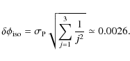
As a consequence the Poissonian noise will be neglected. Following Alard (2009) Sect. 4.6.3, the error on the reconstruction of the potential iso-contours
.
As a consequence the Poissonian noise will be neglected. Following Alard (2009) Sect. 4.6.3, the error on the reconstruction of the potential iso-contours
![]() is
is
![\begin{figure}
\par\includegraphics[angle=0,width=8cm,clip]{13398f9.ps}
\end{figure}](/articles/aa/full_html/2010/05/aa13398-09/img53.png)
|
Figure 9: Histogram of normalized residual (black curve) superposed to the Gaussian expectation (red curve). |
| Open with DEXTER | |
6 Properties of the lens
The perturbative expansion is related directly to the properties of the lens potential. In particular Eq. (C.1) in Alard (2009) relates f0 to the potential isocontours.
6.1 Potential isocontours
The solution of the perturbative lens equation (Eq. (5)) depends
on
![]() ,
i=0,1, and x0, y0, the source impact parameters. The potential isocontour is related
to f0 by the equation
,
i=0,1, and x0, y0, the source impact parameters. The potential isocontour is related
to f0 by the equation
![]() (see Alard 2009, Eq. (C.1)). Since only
(see Alard 2009, Eq. (C.1)). Since only
![]() is known, and since the impact parameters are unknown the first order Fourier terms of f0 are unknown.
The first order Fourier terms correspond to the centering of the potential and do not affect the shape
of the potential isocontour (see Alard 2009, Sect. 6). As a
consequence the shape of the potential isocontours will be computed
with the Fourier expansion of
is known, and since the impact parameters are unknown the first order Fourier terms of f0 are unknown.
The first order Fourier terms correspond to the centering of the potential and do not affect the shape
of the potential isocontour (see Alard 2009, Sect. 6). As a
consequence the shape of the potential isocontours will be computed
with the Fourier expansion of
![]() from order two
to the maximum order (order three). However, the
inner potential isocontour does not depend on the impact parameters, as
a consequence of which the relevant first order terms are meaningful. But the
corresponding terms are very small, indicating that the center of the
inner potential isocontour is very close to the center of light.
An important asset of the singular
perturbative approach is that the inner and outer contribution of the mass
distribution to the
potential can be separated. The potential generated by the lens
projected density inside the critical circle corresponds to the
coefficients an and bn in the expansion of the potential (see
Eqs. (B.1) and (B.2) in Alard 2009). The potential generated by the the projected density outside the critical circle corresponds to cn and dn. Equation (B.3) in Alard (2009) relates the Fourier expansion of the
perturbative fields to an, bn, cn and dn. As a consequence
it is possible to reconstruct the potential corresponding to the
projected density within and outside the critical circle.
The potential near the critical circle is dominated by the outer
contribution (see Fig. 10). Furthermore, the shape of the inner
and outer potential are not the same. Both the ellipticity and orientation of
the inner mass are very different. Using the second order
Fourier terms it is straightforward to estimate the elliptical
parameters for the inner and outer potential. The elliptical contour
equation in a coordinate system aligned with the ellipse axis reads
from order two
to the maximum order (order three). However, the
inner potential isocontour does not depend on the impact parameters, as
a consequence of which the relevant first order terms are meaningful. But the
corresponding terms are very small, indicating that the center of the
inner potential isocontour is very close to the center of light.
An important asset of the singular
perturbative approach is that the inner and outer contribution of the mass
distribution to the
potential can be separated. The potential generated by the lens
projected density inside the critical circle corresponds to the
coefficients an and bn in the expansion of the potential (see
Eqs. (B.1) and (B.2) in Alard 2009). The potential generated by the the projected density outside the critical circle corresponds to cn and dn. Equation (B.3) in Alard (2009) relates the Fourier expansion of the
perturbative fields to an, bn, cn and dn. As a consequence
it is possible to reconstruct the potential corresponding to the
projected density within and outside the critical circle.
The potential near the critical circle is dominated by the outer
contribution (see Fig. 10). Furthermore, the shape of the inner
and outer potential are not the same. Both the ellipticity and orientation of
the inner mass are very different. Using the second order
Fourier terms it is straightforward to estimate the elliptical
parameters for the inner and outer potential. The elliptical contour
equation in a coordinate system aligned with the ellipse axis reads
To first order in
Considering that
An identification with the potential isocontour equation
![\begin{figure}
\par\includegraphics[width=8.5cm,clip]{13398f10.ps}\vspace*{3mm}
\end{figure}](/articles/aa/full_html/2010/05/aa13398-09/img67.png)
|
Figure 10: The potential isocontours. The black curve corresponds to the potential generated by the whole mass distribution, the blue curve corresponds to the potential generated by the outer projected mass distribution and the red curve corresponds the potential generated by the projected mass distribution inside the critical circle. Note that the first order Fourier terms have not been included in the expansion (due to a degeneracy with the impact parameters). As a consequence the position of the contour center is unknown for the outer distribution. In this plot the direction of the vertical axis is parallel to the North (North is up and East is left). To improve the readability of the plot, the amplitude of the noncircular distortion has been exaggerated (by a factor of five). |
| Open with DEXTER | |
6.2 Comparison to observational properties of the lens
It is interesting to compare the inner potential isocontour with the isocontours of the galaxy situated at the center of the lens. To estimate the photometric properties of the lens a Sersic profile was fitted to the light distribution. A similar procedure was already performed by Tu et al. (2009). The surface mass density profile is identical to Tu et al. (2009), Eq. (1), except that the quantity6.2.1 Mass distribution outside the critical circle
Let us now turn to the contribution of the outer
projected distribution to the potential. Tu et al. (2009) pointed out
that the central galaxy is close to a group of galaxies observed by Geach
et al. (2007). The great difference between the outer and inner
mass distribution is due to the influence of this group on the outer
component. A simple model considers two isothermal components
for the central galaxy dark matter halo and for the mass of the group.
Let us assume that these two isothermal components have a
velocity respectively dispersion of ![]() and
and ![]() .
The potential for an isothermal system then reads
.
The potential for an isothermal system then reads
![]() ,
where c0 is a
constant. The central galaxy is very close to the center of the
coordinate system, thus
,
where c0 is a
constant. The central galaxy is very close to the center of the
coordinate system, thus

In a coordinate system where the center of the group is on the abscissa axis at a distance r1 ll 1, the potential of the group reads
The critical condition implies that
![]() ,
thus
,
thus
![]() ,
and as a consequence
,
and as a consequence
To estimate the contribution of the group to the field f0,
we will evaluate
![]() at r=1. To second order in
at r=1. To second order in
![]()
The coefficient of the second order Fourier term of f0 at r=1 is
![]() .
An identification with the
isocontour equation (Eq. (6)) shows that
.
An identification with the
isocontour equation (Eq. (6)) shows that

In the former section it was estimated that
![]() ,
and
adopting the position of the center of the group proposed by Tu et al.
(2009),
,
and
adopting the position of the center of the group proposed by Tu et al.
(2009),
![]() (in units of the critical radius). As a consequence,
(in units of the critical radius). As a consequence,
![]() .
Geach et al. estimate that
.
Geach et al. estimate that
![]() km s-1 from the
km s-1 from the
![]() relation and
relation and
![]() km s-1 from the X-ray temperature. Tu et al. (2009)
estimate from photometric data that
km s-1 from the X-ray temperature. Tu et al. (2009)
estimate from photometric data that
![]() .
Assuming that the mass is dominated by the
dark halo, this means respectively
.
Assuming that the mass is dominated by the
dark halo, this means respectively
![]() and
and
![]() .
Both value are compatible
with
.
Both value are compatible
with
![]() inferred from the outer
contribution to the potential estimated using the perturbative approach.
Let us now estimate the compatibility between the inclination
angles. The group center is situated in a direction at
inferred from the outer
contribution to the potential estimated using the perturbative approach.
Let us now estimate the compatibility between the inclination
angles. The group center is situated in a direction at
![]() from the abscissa axis. Since the uncertainty of the group
center position is 10 arcsecs (Tu et al. 2009) this translates into an error in
from the abscissa axis. Since the uncertainty of the group
center position is 10 arcsecs (Tu et al. 2009) this translates into an error in ![]() of
of
![]() .
This angle should match the inclination angle of the elliptical contour of the outer potential which is
.
This angle should match the inclination angle of the elliptical contour of the outer potential which is
![]() .
Considering the errors, these two angles
are consistent.
.
Considering the errors, these two angles
are consistent.
7 Discussion
The reconstruction of the lens SL2S02176-0513 with the perturbative method indicates that the gravitational field in this lens is dominated by an outer contribution from a nearby group of galaxies. The separation of the inner and outer potential contribution using the perturbative method is free of any assumptions. Furthermore the perturbative analysis shows that the inner potential contribution is small but statistically significant. The orientation of the inner potential isocontour is consistent with the shape of the central galaxy luminosity contours, which illustrates the accuracy of the perturbative re-construction. The outer potential isocontour reconstructed with the perturbative method is consistent with the perturbation introduced by the group of galaxies. Both the ellipticity and orientation match the group properties. The analysis of this gravitational lens demonstrates the ability of the perturbative approach to separate the inner and outer mass contribution to the potential without making any particular assumptions. This lens is very special since the outer contribution to the potential is well identified and dominates other contributions to the outer potential. For other lenses the identification of the perturbators situated outside the critical radius is generally not obvious, and with conventional methods the ability to reconstruct the proper lens potential is compromised. Since the perturbative approach does not contain these flaws, and as the inner and outer contribution to the potential can be separated it is clear, that an unbiased reconstruction of the lens properties can be performed. This ability of the perturbative method to reconstruct the inner properties of the lens are especially useful to interpret complex gravitational lenses (see Alard 2009). This analysis will be also very useful in the statistical analysis of the perturbation introduced by substructures in dark matter halos (see Alard 2008; Peirani et al. 2008).
AcknowledgementsThis work is based on HST data, credited to STScI and prepared for NASA under Contract NAS 5-26555.
References
- Alard, C. 2000, A&AS, 144, 363 [NASA ADS] [CrossRef] [EDP Sciences] [Google Scholar]
- Alard, C. 2007, MNRAS, 382, L58 [NASA ADS] [Google Scholar]
- Alard, C. 2008, MNRAS, 388, 375 [NASA ADS] [CrossRef] [Google Scholar]
- Alard, C. 2009, A&A, 506, 609 [NASA ADS] [CrossRef] [EDP Sciences] [Google Scholar]
- Alard, C., & Lupton, R. 1998, ApJ, 503, 325 [NASA ADS] [CrossRef] [Google Scholar]
- Bartelmann, M., & Meneghetti, M. 2004, A&A, 418, 413 [NASA ADS] [CrossRef] [EDP Sciences] [Google Scholar]
- Blandford, R. D., & Kovner, I. 1988, Phys. Rev. A, 38, 4028 [NASA ADS] [CrossRef] [PubMed] [Google Scholar]
- Clowe, D., Bradac, M., Gonzalez, A., et al. 2006, ApJ, 648, L109 [NASA ADS] [CrossRef] [Google Scholar]
- Geach, J., Simpson, C., Rawlings, S., Read, A. M., & Watson, M. 2007, MNRAS, 381, 1369 [NASA ADS] [CrossRef] [Google Scholar]
- Krist, J. 1995, ASPC, 77, 349 [Google Scholar]
- Nelder, J., & Mead, R. 1965, Comp. J., 7, 308 [Google Scholar]
- Saha, P., & Williams, L. 2006, ApJ, 653, 936S [NASA ADS] [CrossRef] [Google Scholar]
- Tu, H., & 9 co-hautors 2009, A&A, 501, 475 [NASA ADS] [CrossRef] [EDP Sciences] [Google Scholar]
- Vegetti, S., & Koopmans, L. 2009, MNRAS, 392, 945 [NASA ADS] [CrossRef] [Google Scholar]
- Zhao, H. S., & Qin, B. 2003, ApJ, 582, 2 [NASA ADS] [CrossRef] [Google Scholar]
All Figures
|
|
Figure 1: The red contours indicate the four bright areas visible in the image of the source formed by the lens. The flux in these areas is similar, which suggests that these area corresponds to the same part of the source plane. The yellow contour indicates a detail associated with the 4 other bright details by Tu et al. (2009). |
| Open with DEXTER | |
| In the text | |
|
|
Figure 2:
The shape of
|
| Open with DEXTER | |
| In the text | |
|
|
Figure 3:
The shape of
|
| Open with DEXTER | |
| In the text | |
|
|
Figure 4:
The raw HST flux in each photometric bands normalized by the total flux
in the three bands. The red line represents the color of the fifth
bright area (yellow contour in Fig. 1),
the other lines represent the color of the other four bright areas
(red contours in Fig. 1). The color line of the fifth bright area
is different at the 4 |
| Open with DEXTER | |
| In the text | |
|
|
Figure 5:
The perturbative solution,
|
| Open with DEXTER | |
| In the text | |
|
|
Figure 6: Perturbative reconstruction of SL2S2176-0513. The HST image is on the upper right, the perturbative reconstruction on the upper left, the subtraction between the perturbative reconstruction and the HST data is on the lower left, the last image presents an image of the source. |
| Open with DEXTER | |
| In the text | |
|
|
Figure 7: The caustic system of the lens (red curve) and the source isocontours (black curve). The parts of the source inside and outside the caustics have different image multiplicity. Most of the images are associated with the two bright source regions situated inside the caustics. The fifth bright spot (yellow contour in Fig. 1) is associated with the lower part of the source situated below the caustic curve, very close to the curve. See Fig. 8 for a local zoom. |
| Open with DEXTER | |
| In the text | |
|
|
Figure 8: A zoom image of the source and caustics. |
| Open with DEXTER | |
| In the text | |
|
|
Figure 9: Histogram of normalized residual (black curve) superposed to the Gaussian expectation (red curve). |
| Open with DEXTER | |
| In the text | |
|
|
Figure 10: The potential isocontours. The black curve corresponds to the potential generated by the whole mass distribution, the blue curve corresponds to the potential generated by the outer projected mass distribution and the red curve corresponds the potential generated by the projected mass distribution inside the critical circle. Note that the first order Fourier terms have not been included in the expansion (due to a degeneracy with the impact parameters). As a consequence the position of the contour center is unknown for the outer distribution. In this plot the direction of the vertical axis is parallel to the North (North is up and East is left). To improve the readability of the plot, the amplitude of the noncircular distortion has been exaggerated (by a factor of five). |
| Open with DEXTER | |
| In the text | |
Copyright ESO 2010
Current usage metrics show cumulative count of Article Views (full-text article views including HTML views, PDF and ePub downloads, according to the available data) and Abstracts Views on Vision4Press platform.
Data correspond to usage on the plateform after 2015. The current usage metrics is available 48-96 hours after online publication and is updated daily on week days.
Initial download of the metrics may take a while.