| Issue |
A&A
Volume 513, April 2010
|
|
|---|---|---|
| Article Number | A14 | |
| Number of page(s) | 9 | |
| Section | Planets and planetary systems | |
| DOI | https://doi.org/10.1051/0004-6361/200912871 | |
| Published online | 15 April 2010 | |
Order statistics and heavy-tailed distributions for planetary perturbations on Oort cloud comets
R. S. Stoica1 - S. Liu1 -
Yu. Davydov1 - M. Fouchard2,3,![]() - A. Vienne2,3 -
G. B. Valsecchi4
- A. Vienne2,3 -
G. B. Valsecchi4
1 - University Lille 1, Laboratoire Paul Painlevé, 59655 Villeneuve d'Ascq Cedex, France
2 - University Lille 1, LAL, 59000 Lille, France
3 - Institut de Mécanique Céleste et Calcul d'Ephémérides, 77 av. Denfert-Rochereau, 75014 Paris, France
4 - INAF - IASF, via Fosso del Cavaliere 100, 00133 Roma, Italy
Received 12 July 2009 / Accepted 19 November 2009
Abstract
Aims. This paper tackles important aspects of comet dynamics
from a statistical point of view. Existing methodology uses numerical
integration to compute planetary perturbations to simulate such
dynamics. This operation is highly computational. It is reasonable to
investigate a way in which a statistical simulation of the
perturbations can be handled more easily.
Methods. The first step to answer such a question is to provide
a statistical study of these perturbations in order to determine their
main features. The statistical tools used are order statistics and
heavy-tailed distributions.
Results. The study carried out indicated a general pattern
exhibited by the perturbations around the orbits of the planets. These
characteristics were validated through statistical testing and a
theoretical study based on the Öpik theory.
Key words: methods: statistical - celestial mechanics - Oort Cloud
1 Introduction
Comet dynamics are among the most difficult phenomena to model in celestial mechanics. Indeed their dynamics is strongly chaotic, which makes individual motions of known comets hardly reproducible for more than a few orbital periods. When the origin of comets is under investigation, one has to fall back on the use of statistical tools in order to model the motion of a huge number of comets supposed to be representative of the actual population. Ideally, statistical modelling should also be reliable on a time scale comparable to the age of the solar system.
Due to their very elongated shapes, comet trajectories are affected by planetary perturbations during close encounters with planets. In particular, the perturbations induced by the major planets are fundamental in determining the evolution of comet trajectories. Consequently, it is of major importance to model these perturbations in a way which is statistically reliable and which needs the shortest computing time.
A direct numerical integration of a six-bodies-restricted problem (Sun, Jupiter, Saturn, Uranus, Neptune, Comet) for each time a comet enters the planetary region of the solar system is not possible due to the cost in computer time.
Looking for an alternative approach, we can take advantage of the fact that planetary perturbations for the Oort cloud comets are uncorrelated. In fact the orbital periods of such comets are so much longer than those of the planets that when the comet returns, the phases of the latter can be taken at random. Thus we can build a synthetic integrator à la Froeschlé and Rickman (Froeschlé & Rickman 1981) to speed up the modeling. The criticism by Fouchard et al. (2003) to such an approach does not apply in the present case because, as was pointed out above, successive planetary perturbations of Oort cloud comets are uncorrelated.
The aim of this paper is to give a statistical description of a large set of planetary perturbations assumed to be representative of those acting on Oort cloud comets entering the planetary region. To this purpose we use order statistics and heavy-tailed distributions.
The rest of this paper is organised as follows. Section 2 is devoted to the presentation of the mechanism producing the data, i.e. the planetary perturbations and the statistical tools used to analyse the data. These tools are order statistics and heavy-tail distributions, which respectively allow the study and the modeling of the data distribution, with special attention to its symmetry, skewness and tail fatness. The obtained results are shown and interpreted in the third section. The results are finally analysed from a more theoretical point of view using the Öpik theory in Sect. 4. The paper closes with conclusions and perspectives.
2 Statistical tools
2.1 Data compilation
By planetary perturbations we mean the variations of the orbital
parameters between their values before entering the planetary region
of the solar system, i.e. the barycentric orbital element of the
osculating cometary orbit
![]() (where q, i,
(where q, i, ![]() ,
,
![]() are the perihelion distance, the
inclination, the argument of perihelion and the longitude of the
ascending node and z=-1/a with a the semi-major axis), and their
final values
are the perihelion distance, the
inclination, the argument of perihelion and the longitude of the
ascending node and z=-1/a with a the semi-major axis), and their
final values
![]() that is either
when the comet is at its aphelion or when it is back on a Keplerian
barycentric orbit.
that is either
when the comet is at its aphelion or when it is back on a Keplerian
barycentric orbit.
Between its initial and final values, the system Sun + Jupiter +
Saturn + Uranus + Neptune + comet is integrated using the RADAU
integrator at the 15th order (Everhart 1985) for a maximum of
2000 yrs. Then the planetary perturbations obtained through this
integration are
![]() .
The details on the numerical experiment used
to perform the integrations may be found in Rickman et al. (2001).
.
The details on the numerical experiment used
to perform the integrations may be found in Rickman et al. (2001).
Repeating the above experiment with a huge number of comets (namely
9 600 000), one gets a set of planetary perturbations. The comets
are chosen with uniform distribution of the perihelion distance
between 0 and 32 AU, the cosine of the ecliptic inclination between -1 and
1 and the argument of perihelion, and the longitude of the ascending node between 0 and ![]() .
The initial mean anomaly is chosen in a way that the
perihelion passage on its initial Keplerian orbit occurs randomly with
a uniform distribution between 500 and 1500 years after the
beginning of the integration.
.
The initial mean anomaly is chosen in a way that the
perihelion passage on its initial Keplerian orbit occurs randomly with
a uniform distribution between 500 and 1500 years after the
beginning of the integration.
In the present study each perturbation is
associated to the couple
![]() because the perturbations are mainly depending
on qi and
because the perturbations are mainly depending
on qi and ![]() (Fernández 1981). Similarly, since the
orbital energy is the main quantity which is affected by the planetary
perturbations, we will consider only these perturbations here.
(Fernández 1981). Similarly, since the
orbital energy is the main quantity which is affected by the planetary
perturbations, we will consider only these perturbations here.
Consequently, our data are composed by a set of triplets
![]() where Z=zf-zi denotes the perturbations of the cometary
orbital energy by the planets, and
where Z=zf-zi denotes the perturbations of the cometary
orbital energy by the planets, and
![]() a point in a
space denoted by K. We call Z the perturbation mark for the remainder of the paper.
a point in a
space denoted by K. We call Z the perturbation mark for the remainder of the paper.
2.2 Exploratory analysis based on order statistics
Let
![]() be a sequence of independent identically
distributed random variables and let
be a sequence of independent identically
distributed random variables and let
![]() be
the corresponding cumulative distribution function. Let us consider
also
be
the corresponding cumulative distribution function. Let us consider
also ![]() ,
the set of permutations on
,
the set of permutations on
![]() .
.
The order statistics of the sample
![]() is the
rearrangement of the sample in increasing order and it is denoted by
is the
rearrangement of the sample in increasing order and it is denoted by
![]() .
Hence
.
Hence
![]() ,
and there exists a random permutation
,
and there exists a random permutation
![]() in the form of
in the form of
Below some classical results from the literature are presented (Delmas & Jourdain 2006; David 1981). If F is continuous, then almost surely
A major characteristic of order statistics is that they allow quantiles approximations. The quantiles are one of the most easy-to-use tools for characterising a probability distribution. In practice, the data distribution can be described by such empirical quantiles.
Two prominent aspects are now presented. The first one shows how to
compute empirical quantiles using order statistics. Let us assume that
F is continuous and that there exists a unique solution zq to the
equation F(z) = q with
![]() .
Clearly, zq is the q-quantile of
F. Let
.
Clearly, zq is the q-quantile of
F. Let
![]() be an integer sequence with
be an integer sequence with
![]() and
and
![]() .
Then the sequence of the empirical quantiles
.
Then the sequence of the empirical quantiles
![]() converges almost surely towards zq.
converges almost surely towards zq.
The second aspect allows the computation of confidence intervals and
hypothesis testing. If Z1 has a continuous probability density
f with
f(zq) > 0 for
![]() and if it is supposed
that
and if it is supposed
that
![]() ,
then
Z(k(n),n) converges in
distribution towards zq as follows:
,
then
Z(k(n),n) converges in
distribution towards zq as follows:

The exploratory analysis we propose for the perturbation data sets is based on the computation of empirical quantiles. There are several reasons motivating such a choice. First, little is known about the prior distribution concerning the perturbation marks, except that they are distributed around zero and that they are uniformly located in K. This implies that very few hypotheses with respect to the data can be made. Clearly, in order to apply such an analysis the only assumptions needed are the conditions of validity for the central limit theorem. From a practical point of view, an empirical quantiles-based analysis allows the checking of the tails, the symmetry and the general spatial pattern of the data distribution. From a theoretical point of view, the mathematics behind this tool allow us a rather rigorous analysis.
2.3 Stable distribution models
Stable laws are a rich class of probability distributions that allow
heavy tails and skewness and have many nice mathematical properties. They
are also known in the literature under the name of ![]() -stable,
stable Paretian or Lévy stable distributions. These models were
introduced by Levy (1925). Below some basic notions and
results on stable distributions are given (Borak et al. 2005; Samorodnitsky & Taqqu 1994; Feller 1971).
-stable,
stable Paretian or Lévy stable distributions. These models were
introduced by Levy (1925). Below some basic notions and
results on stable distributions are given (Borak et al. 2005; Samorodnitsky & Taqqu 1994; Feller 1971).
A random variable Z has a stable distribution if for any
A,B>0, there is a C>0 and
![]() in a way that
in a way that
where Z1 and Z2 are independent copies of Z, and ``
A stable distribution is characterised by four parameters
![]() ,
,
![]() ,
,
![]() and
and
![]() and it is denoted by
and it is denoted by
![]() .
The role of each parameter is as
follows:
.
The role of each parameter is as
follows: ![]() determines the rate at which the distribution
tail converges to zero,
determines the rate at which the distribution
tail converges to zero, ![]() controls the skewness of the
distribution, whereas
controls the skewness of the
distribution, whereas ![]() and
and ![]() are the scale and shift
parameters, respectively. Figure 1 shows the
influence of these parameters on the distribution shape.
are the scale and shift
parameters, respectively. Figure 1 shows the
influence of these parameters on the distribution shape.
![\begin{figure}
\par a)\includegraphics[width=7.25cm,height=5.25cm,clip]{FIGURES/...
...ludegraphics[width=7cm,height=5.25cm,clip]{FIGURES/stablepdfsd.eps}
\end{figure}](/articles/aa/full_html/2010/05/aa12871-09/img52.png)
|
Figure 1:
Influence of the parameters on the shape of a stable distribution: a) |
| Open with DEXTER | |
The linear transformation of a stable random variable is also a stable
variable. If
![]() ,
then
,
then
![]() for any
for any
![]() and
and
![]() for any
for any
![]() .
The
distribution is Gaussian if
.
The
distribution is Gaussian if ![]() .
The stable variable with
.
The stable variable with
![]() has an infinite variance, and the corresponding distribution
tails are asymptotically equivalent to a Pareto
law (Skorokhod 1961). More precisely
has an infinite variance, and the corresponding distribution
tails are asymptotically equivalent to a Pareto
law (Skorokhod 1961). More precisely
where
One of the technical difficulties in the study of stable distribution is that except for a few cases (Gaussian, Cauchy and Lévy), there is no explicit form for the densities. The characteristic function can be used instead to describe the distribution. There exist numerical methods able to approximate the probability density and the cumulative distribution functions (Nolan 1997). Simulation algorithms for sampling stable distribution can be found in Borak et al. (2005); Chambers et al. (1976).
Due to the previous considerations, parameter estimation is still an
open and challenging problem. Several methods are available in the
literature (Press 1972; McCulloch 1986; Fama & Roll 1971; Mittnik et al. 1999; Nolan 2001). Nevertheless,
these methods all have the same drawback in the sense that the data
is supposed to be a sample of a stable law. It is a well known fact
that if the data come from a different distribution, the inference of
the tail index may be strongly misleading. A solution to this problem
is to estimate the tail exponent (Hill 1975) and then estimate
distribution parameters if
![]() .
.
Still, there remains the problem of the parameter estimation
whenever the tail exponent is greater than 2. Under these
circumstances, distributions with regularly varying tails can be
considered. A random variable has a distribution with regularly
varying tails of an index of
![]() if
if
![]() and a slowly varying function L, i.e.
and a slowly varying function L, i.e.
![]() for any
for any
![]() ,
so that
,
so that
It is important to notice that the conditions (2) can be obtained from (3) whenever
The parameter estimation algorithm proposed
by Davydov & Paulauskas (2004,1999) is constructed under the assumption
that the sample distribution has the asymptotic
property (2). The algorithm gives three estimated values
![]() .
The
.
The
![]() can be computed easily whenever
can be computed easily whenever
![]() ,
by
approximating it using the empirical mean of the samples. This
parameter estimation method can be used for stable distribution and in
this case,
,
by
approximating it using the empirical mean of the samples. This
parameter estimation method can be used for stable distribution and in
this case,
![]() should indicate positive values lower
than 2. At the same time, the strong point of the method is that it
can be used for data which do not follow stable distributions. In this case
the data distribution is assumed to have regularly varying tails. The
weak point of this algorithm is that in this case it does not give
indications concerning the body of the distribution.
Nevertheless this method allows in both cases a rather complete characterisation of a
wide panel of probability distributions. The code implementing the
algorithm is available just by simple demand to the authors.
should indicate positive values lower
than 2. At the same time, the strong point of the method is that it
can be used for data which do not follow stable distributions. In this case
the data distribution is assumed to have regularly varying tails. The
weak point of this algorithm is that in this case it does not give
indications concerning the body of the distribution.
Nevertheless this method allows in both cases a rather complete characterisation of a
wide panel of probability distributions. The code implementing the
algorithm is available just by simple demand to the authors.
![\begin{figure}
\par\subfigure[]{\includegraphics[width=7cm,clip]{gray-tail01_08_...
...re[]{\includegraphics[width=7cm,clip]{gray-tail25_32_heavy.eps} }\end{figure}](/articles/aa/full_html/2010/05/aa12871-09/img81.png)
|
Figure 2:
Empirical quantiles based difference indicator
|
| Open with DEXTER | |
3 Results
3.1 Empirical quantiles
The lack of stationarity of the perturbation marks imposes the
partitioning of the location space in a finite number of cells. Let us
consider such a partition
![]() .
The cells Ki are
disjoint, and they all have the same volume. The size of the volume has to
be big enough in order to contain a sufficient number of
perturbations. At the same time, the volume has to be small enough to
allow for stationarity assumptions for the perturbation marks inside a
cell. After several trial and errors, we have opted for a partition
made of square cells Ki, all having the same volume
.
The cells Ki are
disjoint, and they all have the same volume. The size of the volume has to
be big enough in order to contain a sufficient number of
perturbations. At the same time, the volume has to be small enough to
allow for stationarity assumptions for the perturbation marks inside a
cell. After several trial and errors, we have opted for a partition
made of square cells Ki, all having the same volume
![]() AU,
so that each cell contains about 1500 perturbations.
AU,
so that each cell contains about 1500 perturbations.
We were interested in three questions concerning the perturbation marks distributions. The first two questions are related to the tails and the symmetry of the data distribution. The third question is related to a more delicate problem. It is a well known fact that the perturbation locations follow an uniform distribution in K. Nevertheless, little is known about the spatial distribution of the perturbation marks, except that they are highly dependent on their corresponding locations. So, the third question to be formulated is the following: do the distributions of the perturbation marks exhibit any pattern depending on the perturbation location?
For this purpose, empirical q-quantiles were computed in each cell. Most of these values indicate that the perturbation marks are distributed around the origin, while no particular spatial pattern is exhibited in the perturbation location space.
On the other hand, the situation is completely different for extreme
q-values such as
0.01,0.05,0.95,0.99. These quantiles indicate
rather important values around the semi-major axis of each
planet. In order to check if these values may reveal heavy tail
distributions, the difference based indicator
![]() was built. The first term of this indicator
represents an empirical q-quantile. The second term is the
theoretical q-quantile of the normal law with mean and standard
deviation given by z0.50 and
0.5(z0.84-z0.16). Hence, for
values of q approaching 1, positive values of the indicator may
suggest heavy-tail behaviour for the data. Clearly, this indicator may
be used also for quantiles approaching 0. In this case, it is the
negative sign that reveals the fatness of the distribution tail.
was built. The first term of this indicator
represents an empirical q-quantile. The second term is the
theoretical q-quantile of the normal law with mean and standard
deviation given by z0.50 and
0.5(z0.84-z0.16). Hence, for
values of q approaching 1, positive values of the indicator may
suggest heavy-tail behaviour for the data. Clearly, this indicator may
be used also for quantiles approaching 0. In this case, it is the
negative sign that reveals the fatness of the distribution tail.
In Fig. 2 the values obtained for the
difference indicator
![]() are shown. It can
be observed that its rather important values appeared whenever the
perturbations are located in the vicinity of a planet orbit. All these
values tend to form a spatial pattern similar to an arrow-like
shape. As it can be observed, this shape is situated around the planet
orbit and points from the right to left. It tends to vanish
when the cosine of the inclination angle approaches -1. The
prominence of this arrow shape clearly depends on the closest planet:
the bigger the planet, the sharper is the arrow-like shape. This can be
observed by looking at the change of values for the
difference indicator with respect to the size of the planet. These
observations fulfil some common sense expectations: the comet
perturbations tend to be more important whenever a comet crosses the
orbit of a giant planet.
are shown. It can
be observed that its rather important values appeared whenever the
perturbations are located in the vicinity of a planet orbit. All these
values tend to form a spatial pattern similar to an arrow-like
shape. As it can be observed, this shape is situated around the planet
orbit and points from the right to left. It tends to vanish
when the cosine of the inclination angle approaches -1. The
prominence of this arrow shape clearly depends on the closest planet:
the bigger the planet, the sharper is the arrow-like shape. This can be
observed by looking at the change of values for the
difference indicator with respect to the size of the planet. These
observations fulfil some common sense expectations: the comet
perturbations tend to be more important whenever a comet crosses the
orbit of a giant planet.
Since these phenomena are observed for extremal q-quantiles, they indicate that the distribution tails may be an important feature for the data. Hence, a statistical model for the data should be able to reproduce these characteristics of the perturbation marks.
Empirical quantiles can be also used in a straightforward way as symmetry indicators of the data distribution. Clearly, by just checking whenever the difference zq - |z1-q| tends to 0, this may suggest a rather symmetric data distribution. Figure 3 shows the computation of such differences for each data cell. The values obtained are rather low all over the studied region. Nevertheless, there are some regions, and especially around the Jupiter's orbit we may suspect the data distributions to be a little bit skewed. Still, since the perturbations have comparatively low numerical values, assessing the symmetry using the proposed indicator has to be done cautiously.
It is reasonable to expect a more reliable answer concerning this question by using a statistical model. Clearly, such a model should be able to reproduce the symmetry of the data distribution as well.
![\begin{figure}
\par\includegraphics[width=8cm,clip]{gray-sym01_08.eps}
\end{figure}](/articles/aa/full_html/2010/05/aa12871-09/img85.png)
|
Figure 3: Exploring the symmetry using empirical quantiles difference z0.99 - |z0.01| for the perturbation marks around Jupiter. Axis are as for Fig. 2. The range interval is [-0.0025,0.0014]. |
| Open with DEXTER | |
The central limit theorem available for the order statistics allows
the construction of an hypothesis test. Since our analysis leads us
towards heavy-tailed distribution models, a
statistical test was performed as a precaution to verify wether a more simple model can
be fit to the data. The normality assumption was considered as the null
hypothesis for the test. The test was performed for the data in each
cell, by considering that the normal distribution parameters are given
by the empirical quantiles as explained previously. The p-values were
computed using a ![]() distribution. In this context, the local
normality assumption for the perturbation marks is globally
rejected. Figure 4 shows the result of testing
the normality of the z0.95 empirical quantile computed around the
Jupiter's orbit.
distribution. In this context, the local
normality assumption for the perturbation marks is globally
rejected. Figure 4 shows the result of testing
the normality of the z0.95 empirical quantile computed around the
Jupiter's orbit.
Indeed, there exist regions where the normality assumptions cannot be rejected for the considered quantile. Still, the regions where this hypothesis is rejected clearly indicate that normality cannot be assumed throughout. Therefore, a parametric statistical model has to be able to reflect this situation and indicate the cases for ``heavy'' or stable distribution tails.
![\begin{figure}
\par\includegraphics[width=8cm,clip]{gray-test01_08.eps}
\end{figure}](/articles/aa/full_html/2010/05/aa12871-09/img86.png)
|
Figure 4: p-values computed to test the normality of the empirical quantiles z0.95 around Jupiter. |
| Open with DEXTER | |
The only parameter used during this exploratory analysis was the partitioning of the location domain K. There is one more question to answer: do the obtained results depend on the patterns exhibited by the data, or they are just a consequence of the partitioning in cells of the data locations? To answer this question, a bootstrap procedure and a permutation test were implemented (Davison & Hinkley 1997).
Bootstrap samples were randomly selected by uniformly
choosing 20%
from the entire perturbations data set. Difference indicators were
computed for this special data set. This operation was repeated
100 times. At the end of the procedure, the empirical means of the
difference indicators were computed. In
Fig. 5a the bootstrap mean of the
indicator
![]() around Jupiter's orbit is
showed. As expected, the same pattern is obtained as in
Fig. 2a: important values are grouped around
the planet's orbit and exhibit an arrow-like shape pointing from
right to left.
around Jupiter's orbit is
showed. As expected, the same pattern is obtained as in
Fig. 2a: important values are grouped around
the planet's orbit and exhibit an arrow-like shape pointing from
right to left.
The permutation test follows the same steps as the bootstrap procedure
except that the perturbations are previously permuted. This means that
all the perturbations are modified as follows: for a given
perturbation the mark is kept while its location is exchanged with
the location of another randomly chosen perturbation. This procedure
should destroy any pre-existing structure in the data. In this case,
we expect that applying a bootstrap procedure on this new data set
will indicate no relevant patterns. In
Fig. 5b the result of such a permutation
test is shown. The experiment was carried out in the vicinity of
Jupiter's orbit. After permuting the perturbations as indicated, the
previously described bootstrap procedure was applied in order to
estimate bootstrap means of the difference indicator
![]() .
The result confirmed our expectations in the
sense that no particular structure or pattern is observed. This
clearly indicates that the analysis results were due mainly to the
original data structure and not to the partitioning of the
perturbations location domain in cells.
.
The result confirmed our expectations in the
sense that no particular structure or pattern is observed. This
clearly indicates that the analysis results were due mainly to the
original data structure and not to the partitioning of the
perturbations location domain in cells.
At the same time, the permutation test is also a verification of the proposed exploratory methodology. This methodology depends on a precision parameter to characterise the hidden structure or pattern exhibited by the data. Still, whenever such a structure does not exist at all, the present method detects nothing.
![\begin{figure}
\par\subfigure[]{\includegraphics[width=7cm,clip]{gray-boot01_08_...
...ure[]{\includegraphics[width=7cm,clip]{gray-perm01_08_heavy.eps} }\end{figure}](/articles/aa/full_html/2010/05/aa12871-09/img87.png)
|
Figure 5:
Validation of the analysis based on the computation of the difference indicator
|
| Open with DEXTER | |
3.2 Inference using heavy-tail distributions
The empirical observations of the perturbation marks distributions indicated fat tails and skewness behaviour. This leptokurtic character of the perturbation distributions was observed especially in the vicinity of the planets'orbits. In response to this empirical evidence heavy-tail distribution modeling was chosen.
The same cell partitioning as for the exploratory analysis is maintained. The previously mentioned algorithm to estimate stable law parameters was run for the data in each cell.
In Fig. 6 the estimation result of the tail
exponent is shown. A region can be clearly observed which is formed by the
cells corresponding to estimated ![]() values lower than 2. This
kind of region may be located around each orbit which corresponds to a big
planet. The shape of this region is less picked than the region
obtained using empirical quantiles. Still, the two results are
coherent. Both results indicate that the heavy-tailed character of the
perturbations distributions exhibits a spatial pattern. This spatial
pattern is located around the orbits of the major planets.
values lower than 2. This
kind of region may be located around each orbit which corresponds to a big
planet. The shape of this region is less picked than the region
obtained using empirical quantiles. Still, the two results are
coherent. Both results indicate that the heavy-tailed character of the
perturbations distributions exhibits a spatial pattern. This spatial
pattern is located around the orbits of the major planets.
![\begin{figure}
\par\subfigure[]{\includegraphics[width=7.3cm,clip]{gray-alpha01_...
...figure[]{\includegraphics[width=7.3cm,clip]{gray-alpha25_32.eps} }\end{figure}](/articles/aa/full_html/2010/05/aa12871-09/img88.png)
|
Figure 6:
Estimation result of the tail exponent |
| Open with DEXTER | |
The skewness of the data distribution can be analysed by looking at the results shown in Fig. 7. Indeed, it can be observed that there are cells containing perturbations following a skewed distribution. The obtained results indicate neither the presence of a pattern by such distributions nor the presence of such a pattern around the orbits of the major planets.
![\begin{figure}
\par\includegraphics[width=8.5cm,clip]{gray-beta01_08.eps}
\end{figure}](/articles/aa/full_html/2010/05/aa12871-09/img89.png)
|
Figure 7:
Estimation result of the skewness parameter |
| Open with DEXTER | |
The estimation results for the ![]() and
and ![]() parameters are
presented in Fig. 8. The scale parameter
indicates how heavy the distribution tails are. It may be observed in
Fig. 8a that the most
important values of
parameters are
presented in Fig. 8. The scale parameter
indicates how heavy the distribution tails are. It may be observed in
Fig. 8a that the most
important values of ![]() tend to form a spatial pattern similar
to the patterns formed by the difference indicator based on order
statistics and the tail exponent, respectively. The results
obtained for the
tend to form a spatial pattern similar
to the patterns formed by the difference indicator based on order
statistics and the tail exponent, respectively. The results
obtained for the ![]() parameter indicate that a shift of the
perturbation may exist around the orbit of the corresponding big
planets.
parameter indicate that a shift of the
perturbation may exist around the orbit of the corresponding big
planets.
![\begin{figure}
\par\subfigure[]{\includegraphics[width=8.5cm,clip]{gray-sigma01_...
...figure[]{\includegraphics[width=8.5cm,clip]{gray-delta01_08.eps} }\end{figure}](/articles/aa/full_html/2010/05/aa12871-09/img90.png)
|
Figure 8:
Estimation result of the scale parameter |
| Open with DEXTER | |
To check these results a statistical test using the central
limit theorem for order statistics was built. This result can
be used to verify if the empirical quantiles from a cell are
coming from the distribution characterised by the parameters
previously estimated. Figure 9 shows the result of a
test verifying that the z0.99 quantiles around the Jupiter's
orbit are originated from a heavy-tail distribution, while the
quantiles outside this region are coming instead from Pareto
distribution. It can be observed that high results for the p-values
are spread around the entire region: for ![]() of the cells we
cannot reject the null hypothesis. This result is obviously a far
better characterisation of the distribution tails of the perturbations
than the test for the normality assumption performed in the preceding
section.
of the cells we
cannot reject the null hypothesis. This result is obviously a far
better characterisation of the distribution tails of the perturbations
than the test for the normality assumption performed in the preceding
section.
| Figure 9: p-values computed to test if the empirical quantiles z0.99 around the Jupiter's orbit are originated from a heavy-tail distribution. |
|
| Open with DEXTER | |
The previous test certifies that the perturbations distributions tails
exhibit a stable or regular variation behaviour. If the perturbations
are close
to the orbit of a big planet they have mainly a stable
behaviour. Figure 10 shows the p-values of
a ![]() -test implemented for the perturbations with an estimated tail
exponent
-test implemented for the perturbations with an estimated tail
exponent
![]() .
This test allows us to check the perturbations
also for their distribution body. It can be observed that in almost
all these regions the assumption of stable distributions is accepted.
.
This test allows us to check the perturbations
also for their distribution body. It can be observed that in almost
all these regions the assumption of stable distributions is accepted.
![\begin{figure}
\par\subfigure[]{\includegraphics[width=6.5cm,height=4.5cm,clip]{...
...cs[width=6.5cm,height=4.5cm,clip]{gray-q25_32_10-chi-stable.eps} }\end{figure}](/articles/aa/full_html/2010/05/aa12871-09/img93.png)
|
Figure 10:
p-values of a |
| Open with DEXTER | |
For the perturbations with a tail exponent greater than 2, an
alternative family of distributions with regularly varying tails was
considered for modelling. Its expressions is given below:
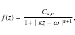
with
The parameter estimation for such distributions was done in several
steps. First, the tail exponent ![]() was obtained from
the previous algorithm. Second, the location parameter
was obtained from
the previous algorithm. Second, the location parameter ![]() was
estimated by the empirical mean of the data samples. Finally, the
normalising constant
was
estimated by the empirical mean of the data samples. Finally, the
normalising constant
![]() and the scale parameter
and the scale parameter
![]() were estimated using the method of moments.
were estimated using the method of moments.
A ![]() statistical test was done for the perturbations with
statistical test was done for the perturbations with
![]() .
The null hypothesis considered was that the
considered perturbations follow a regularly varying tail
distribution (4) with parameters given by the
previously described procedure. The obtained p-values are shown in
Fig. 11. It can be noticed that in the majority of
considered cells the null hypothesis is accepted.
.
The null hypothesis considered was that the
considered perturbations follow a regularly varying tail
distribution (4) with parameters given by the
previously described procedure. The obtained p-values are shown in
Fig. 11. It can be noticed that in the majority of
considered cells the null hypothesis is accepted.
![\begin{figure}
\par\subfigure[]{\includegraphics[width=6.5cm,height=4.5cm,clip]{...
...idth=6.5cm,height=4.5cm,clip]{gray-q25_32_10-chi-vr-nonstab.eps} }\end{figure}](/articles/aa/full_html/2010/05/aa12871-09/img97.png)
|
Figure 11:
p-values of a |
| Open with DEXTER | |
4 Discussion and interpretation
Some of the features present in the Figures can be explained in the framework of the analytical theory of close encounters (Greenberg et al. 1988; Valsecchi & Manara 1997; Opik 1976; Carusi et al. 1990).
Let us consider the magnitude of the perturbations in the vicinity of
a=aJ=5.2 AU (Jupiter). The
colour coding of Fig. 2 is related to the magnitude P of the perturbation, corresponding to
where a and h are the orbital semi-major axis and the orbital energy of the heliocentric Keplerian motion of the comet respectively. The subscripts i and f stand, respectively, for initial and final, i.e., before and after the interaction with Jupiter.
Perturbations at planetary encounters are characterised by large and in general asymmetric tails, as was shown by various authors (Everhart 1969; Oikawa & Everhart 1979; Froeschlé & Rickman 1981); an analytical explanation of these features was given by Carusi et al. (1990) and by Valsecchi et al. (2000), and the consequences on the orbital evolution of comets was discussed by Valsecchi & Manara (1997).
We now consider the case of parabolic initial orbits (our orbits are in fact very close to parabolic), and discuss the conditions under which we can expect asymmetric tails in the energy perturbation distributions.
The condition for the tails of the energy perturbation distribution to be symmetric is (Valsecchi et al. 2000; Carusi et al. 1990):

where we have for a parabolic orbit:

where ap is the orbital semi-major axis of the planet encountered, and U is the planetocentric velocity of the comet at encounter, in units of the orbital velocity of the planet itself. Making the appropriate substitutions, the condition

Anyway, the finite size of the available perturbation sample must be taken into account, as the tails would become sufficiently populated to show any asymmetry only for very large samples.
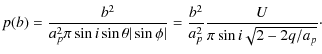
Turning our attention now more generally to the tails of the energy perturbation
distributions, we consider that in different regions of the q-![]() plane the probability p for
the comet on a parabolic orbit to pass within a given unperturbed minimum distance b from
the planet (the so-called impact parameter) would be, according to Opik (1976)
plane the probability p for
the comet on a parabolic orbit to pass within a given unperturbed minimum distance b from
the planet (the so-called impact parameter) would be, according to Opik (1976)
We note that p(b) can also be considered to be the probability with which the comet passes within any circle of a given radius b on the target plane (the plane centred on the planet, and perpendicular to the unperturbed planetocentric velocity of the comet).
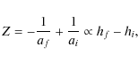
As for the size of the perturbation, Valsecchi et al. (2000) show that, in the target plane, the locus of points
through which the comet has to pass in order to undergo an energy perturbation

(where ai and af are the semi-major axes of the orbit before and after the encounter with the planet) is a circle of radius

where, for a pre-encounter parabolic orbit,

in our case, in which ap/ai=0 and z=-ap/af, this radius is:

Thus, the probability of an energy perturbation of a size equal or greater than z is proportional to the surface of the circle of radius R(z).
Moreover, as noted above, the probability that a comet passes within a circle of a given radius, say R(z), on the target plane can be computed using Öpik's expression (6); we therefore conclude that the probability P(z) that the comet undergoes an energy perturbation of a size equal or greater than z is
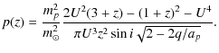
Equation (7) may be inverted to derive the value z of the energy perturbation for which the probability to have a perturbation greater in absolute value than z is equal to a given p. We obtain two solutions, z+ and z-, one for the positive perturbations and one for the negative ones. Each solution is given by

with
Figure 12 shows the level curves of z+ for p=0.01, which is consistant with Fig. 2. As can be seen, the main features of Fig. 2 are reproduced. The arrow-like shape observed during the statistical study can be now observed on the definition domain imposed by the definition of z+. This strenghtens our interpretation of the features of Fig. 2 as due to the geometry of close approaches described by the Öpik theory.
![\begin{figure}
\par\includegraphics[angle=270,width=7.2cm,clip]{level_curves.eps}
\end{figure}](/articles/aa/full_html/2010/05/aa12871-09/img115.png)
|
Figure 12: Level curves of z+ around the semi-major axis of Jupiter. The level of each curve is indicated on the figure. |
| Open with DEXTER | |
5 Conclusion and perspectives
In this paper a statistical study of the planetary perturbations on Oort cloud comets was carried out. The exploratory analysis of the perturbation distributions based on order statistics indicated the tail behaviour as a determining feature. Following this idea, parametric inference for heavy-tail distributions was implemented. The obtained results indicated that the perturbations follow heavy-tail stable distributions which are not always symmetric while tending to form a spatial pattern. This pattern is shaped arrow-like and is situated around the orbits of the major planets. A theoretical study was carried out, and it was observed that this pattern is similar to the theoretical curves derived from the Öpik theory. The perturbations outside this arrow-shaped region were not exhibiting a stable character and they were modelled by a family of distributions with regularly varying tails. In both cases, stable and non-stable distributions, the modelling choices were confirmed by a statistical test.
Clearly, these choices and the estimation parameter estimation procedures can be further improved. Nevertheless, the obtained results give good indications and also good reasons for developing a probabilistic methodology able to simulate such planetary perturbations.
AcknowledgementsThe authors are grateful to Alain Noullez for very useful comments and remarks. They are also gratful to John J. Matese, the referee of the paper, for his helpful comments. Part of this research was supported by the University of Lille 1 through the financial BQR program.
References
- Borak, S., Härdle, W., & Weron, R. 2005, in Statistical tools for finance and insurance, ed. P. Cizek, W. Härdle, & R. Weron, 21, Springer [Google Scholar]
- Carusi, A., Valsechi, G. B., & Greenberg, R. 1990, Celestial Mechanics and Dynamical Astronomy, 49, 111 [Google Scholar]
- Chambers, J., Mallows, C., & Stuck, B. 1976, Journal of the American Statistical Association, 70, 340 [CrossRef] [MathSciNet] [Google Scholar]
- David, H. A. 1981, Order statistics (John Wiley and Sons) [Google Scholar]
- Davison, A. C., & Hinkley, D. V. 1997, Bootstrap methods and their application (Cambrdige University Press) [Google Scholar]
- Davydov, Y., & Paulauskas, V. 1999, Acta Applicandae Mathematicae, 58, 107 [CrossRef] [Google Scholar]
- Davydov, Y., & Paulauskas, V. 2004, Fields Institute Communications, 44, 127 [Google Scholar]
- Delmas, J.-F., & Jourdain, B. 2006, Mathématiques et Applications (SMAI), 57, Modèles aléatoires. Application aux sciences de l'ingénieur et du vivant (Springer) [Google Scholar]
- Everhart, E. 1969, AJ, 74, 735 [NASA ADS] [CrossRef] [Google Scholar]
- Everhart, E. 1985, in Dynamics of Comets: Their Origin and Evolution, ed. A. Carusi & G. B. Valsecchi, ASSL, 115, IAU Colloq. 83:185 [Google Scholar]
- Fama, E., & Roll, R. 1971, Journal of the American Statistical Association, 66, 331 [CrossRef] [Google Scholar]
- Feller, W. 1971, An introduction to probability theory and its applications - II (Wiley) [Google Scholar]
- Fernández, J. 1981, A&A, 96, 26 [NASA ADS] [Google Scholar]
- Fouchard, M., Froeschlé, C., & Valsecchi, G. B. 2003, MNRAS, 344, 1283 [NASA ADS] [CrossRef] [Google Scholar]
- Froeschlé, C., & Rickman, H. 1981, Icarus, 46, 400 [NASA ADS] [CrossRef] [Google Scholar]
- Greenberg, R., Carusi, A., & Valsecchi, G. B. 1988, Icarus, 75, 1 [NASA ADS] [CrossRef] [Google Scholar]
- Hill, B. M. 1975, Annals of Statistics, 3, 1163 [Google Scholar]
- Levy, P. 1925, Calcul des probabilités (Gauthier Villars) [Google Scholar]
- McCulloch, J. H. 1986, Communications in Statistics - Simulation and Computation, 15, 1109 [Google Scholar]
- Mittnik, S., Doganoglu, T., & Chenyao, D. 1999, Mathematical and Computer Modelling, 29, 235 [CrossRef] [Google Scholar]
- Nolan, J. P. 1997, Communications in Statistics - Stochastic Models, 13, 759 [Google Scholar]
- Nolan, J. P. 2001, in Lévy Processes [Google Scholar]
- Oikawa, S., & Everhart, E. 1979, AJ, 84, 134 [NASA ADS] [CrossRef] [Google Scholar]
- Opik, E. J. 1976, Interplanetary encounters: close-range gravitational interactions, ed. E. J. Opik [Google Scholar]
- Press, S. J. 1972, Journal of the American Statistical Association, 67, 842 [CrossRef] [Google Scholar]
- Rickman, H., Valsecchi, G. B., & Froeschlé, C. 2001, MNRAS, 325, 1303 [NASA ADS] [CrossRef] [Google Scholar]
- Samorodnitsky, G., & Taqqu, M. S. 1994, Stable non-Gaussian random processes: stochastic models with infinite variance (Chapman & Hall/CRC) [Google Scholar]
- Skorokhod, A. 1961, in Selected Translations in Mathematical Statistics and Probability 1, 157 [Google Scholar]
- Valsecchi, A., & Manara, G. B. 1997, A&A, 323, 986 [NASA ADS] [Google Scholar]
- Valsecchi, G. B., Milani, A., Gronchi, G. F., et al. 2000, Celestial Mechanics and Dynamical Astronomy, 78, 83 [Google Scholar]
Footnotes
All Figures
|
|
Figure 1:
Influence of the parameters on the shape of a stable distribution: a) |
| Open with DEXTER | |
| In the text | |
|
|
Figure 2:
Empirical quantiles based difference indicator
|
| Open with DEXTER | |
| In the text | |
|
|
Figure 3: Exploring the symmetry using empirical quantiles difference z0.99 - |z0.01| for the perturbation marks around Jupiter. Axis are as for Fig. 2. The range interval is [-0.0025,0.0014]. |
| Open with DEXTER | |
| In the text | |
|
|
Figure 4: p-values computed to test the normality of the empirical quantiles z0.95 around Jupiter. |
| Open with DEXTER | |
| In the text | |
|
|
Figure 5:
Validation of the analysis based on the computation of the difference indicator
|
| Open with DEXTER | |
| In the text | |
|
|
Figure 6:
Estimation result of the tail exponent |
| Open with DEXTER | |
| In the text | |
|
|
Figure 7:
Estimation result of the skewness parameter |
| Open with DEXTER | |
| In the text | |
|
|
Figure 8:
Estimation result of the scale parameter |
| Open with DEXTER | |
| In the text | |
| |
Figure 9: p-values computed to test if the empirical quantiles z0.99 around the Jupiter's orbit are originated from a heavy-tail distribution. |
| Open with DEXTER | |
| In the text | |
|
|
Figure 10:
p-values of a |
| Open with DEXTER | |
| In the text | |
|
|
Figure 11:
p-values of a |
| Open with DEXTER | |
| In the text | |
|
|
Figure 12: Level curves of z+ around the semi-major axis of Jupiter. The level of each curve is indicated on the figure. |
| Open with DEXTER | |
| In the text | |
Copyright ESO 2010
Current usage metrics show cumulative count of Article Views (full-text article views including HTML views, PDF and ePub downloads, according to the available data) and Abstracts Views on Vision4Press platform.
Data correspond to usage on the plateform after 2015. The current usage metrics is available 48-96 hours after online publication and is updated daily on week days.
Initial download of the metrics may take a while.