| Issue |
A&A
Volume 513, April 2010
|
|
|---|---|---|
| Article Number | A52 | |
| Number of page(s) | 30 | |
| Section | Extragalactic astronomy | |
| DOI | https://doi.org/10.1051/0004-6361/200912482 | |
| Published online | 27 April 2010 | |
The globular cluster system of
NGC 1399![[*]](/icons/foot_motif.png) ,,
,,
V. dynamics of the cluster system out to 80 kpc
Y. Schuberth1,2 - T. Richtler2 - M. Hilker3 - B. Dirsch2 - L. P. Bassino4 - A. J. Romanowsky5,2 - L. Infante6
1 - Argelander-Institut für Astronomie, Universität Bonn, Auf dem Hügel
71, 53121 Bonn, Germany
2 - Universidad de Concepción, Departamento de Astronomia, Casilla
160-C, Concepción, Chile
3 - European Southern Observatory, Karl-Schwarzschild-Str. 2,
85748 Garching, Germany
4 - Facultad de Ciencias Astronómicas y Geofísicas, Universidad
Nacional de La Plata, Paseo del Bosque S/N, 1900-La Plata, Argentina;
and Instituto de Astrofísica de La Plata (CCT La Plata -
CONICET - UNLP)
5 - UCO/Lick Observatory, University of California, Santa Cruz, CA
95064, USA
6 - Departamento de Astronomía y Astrofísica, Pontificia Universidad
Católica de Chile, Casilla 306, Santiago 22, Chile
Received 13 May 2009 / Accepted 16 October 2009
Abstract
Globular clusters (GCs) are tracers of the gravitational
potential of their host galaxies. Moreover, their kinematic properties
may provide clues for understanding the formation of GC systems and
their host galaxies. We use the largest set of GC velocities obtained
so far of any elliptical galaxy to revise and extend the previous
investigations (Richtler et al. 2004) of the dynamics
of NGC 1399,
the central dominant galaxy of the nearby Fornax cluster of galaxies.
The GC velocities are used to study the kinematics,
their relation with population properties, and the dark matter halo of
NGC 1399.
We have obtained 477 new medium-resolution spectra (of these, 292 are
spectra from 265 individual GCs, 241 of which are not in the previous
data set). with the VLT FORS 2 and Gemini South GMOS
multi-object spectrographs. We revise velocities for the old spectra
and measure velocities for the new spectra, using the same templates to
obtain an homogeneously treated data set. Our entire sample now
comprises velocities for almost 700 GCs
with projected galactocentric radii between 6 and 100 kpc. In
addition, we use velocities of GCs at larger distances published
elsewhere. Combining the kinematic data with wide-field photometric
Washington data, we study the kinematics of the metal-poor and
metal-rich subpopulations. We discuss in detail the velocity
dispersions of subsamples and perform spherical Jeans modelling.
The most important results are: the red GCs resemble the stellar field population of NGC 1399 in the region of overlap. The blue GCs behave kinematically more erratic. Both subpopulations are kinematically distinct and do not show a smooth transition. It is not possible to find a common dark halo which reproduces simultaneously the properties of both red and blue GCs. Some velocities of blue GCs are only to be explained by orbits with very large apogalactic distances, thus indicating a contamination with GCs which belong to the entire Fornax cluster rather than to NGC 1399. Also, stripped GCs from nearby elliptical galaxies, particularly NGC 1404, may contaminate the blue sample.
We argue in favour of a scenario in which the majority of the blue cluster population has been accreted during the assembly of the Fornax cluster. The red cluster population shares the dynamical history of the galaxy itself. Therefore we recommend to use a dark halo based on the red GCs alone.
The dark halo which fits best is marginally less massive than the halo quoted previously. The comparison with X-ray analyses is satisfactory in the inner regions, but without showing evidence for a transition from a galaxy to a cluster halo, as suggested by X-ray work.
Key words: galaxies: elliptical and lenticular, cD - galaxies: kinematics and dynamics - galaxies: individual: NGC 1399
1 Introduction
1.1 The globular cluster systems of central elliptical galaxies
Shortly after M 87 revealed its rich globular cluster system (GCS) (Baum 1955; Racine 1968) it became obvious that bright ellipticals in general host globular clusters in much larger numbers than spiral galaxies (Harris & Racine 1979). Moreover, the richest GCSs are found for elliptical galaxies in the centres of galaxy clusters, for which M 87 in the Virgo cluster and NGC 1399 in the Fornax cluster are the nearest examples. For recent reviews of the field, see Brodie & Strader (2006), and Richtler (2006).
The galaxy cluster environment may act in different ways to produce these very populous GCSs. Firstly, there is the paradigm of giant elliptical galaxy formation by the merging of disk galaxies (e.g. Toomre 1977; Renzini 2006). That early-type galaxies can form through mergers is evident by the identification of merger remnants and many kinematical irregularities in elliptical galaxies (counter-rotating cores, accreted dust and molecular rings).
In fact, starting from the bimodal colour distribution of GCs in some giant ellipticals, Ashman & Zepf (1992) predicted the efficient formation of GCs in spiral-spiral mergers, before this was confirmed observationally (Schweizer & Seitzer 1993). In their scenario, the blue clusters are the metal-poor GCSs of the pre-merger components while the red (metal-rich) GCs are formed in the material which has been enriched in the starbursts accompanying the early merger (gaseous merger model).
However, Forbes et al. (1997) pointed out that the large number of metal-poor GCs found around giant ellipticals cannot be explained by the gaseous merger model. These authors proposed a ``multi-phase collapse model'' in which the blue GCs are created in a pre-galactic phase along with a relatively low number of metal-poor field stars. The majority of field stars, i.e. the galaxy itself and the red GCs, are then formed from the enriched gas in a secondary star formation epoch. This scenario is also supported by the findings of Spitler et al. (2008) who studied an updated sample of 25 galaxies spanning a large range of masses, morphological types and environments. They confirmed that the spirals generally show a lower fraction of GCs normalised to host galaxy stellar mass than massive ellipticals, thus ruling out the possibility that the GCSs of massive ellipticals are formed through major wet mergers. Further, Spitler et al. suggest that the number of GCs per unit halo mass is constant - thus extending the work by Blakeslee et al. (1997) who found that in the case of central cluster galaxies the number of GCs scales with the cluster mass. These are findings which point towards an early formation of the GCs.
In some scenarios (e.g. Côté et al. 1998,2002; Beasley et al. 2002; Hilker et al. 1999), the accretion of mostly metal-poor GCs is responsible for the richness of the GCSs of central giant ellipticals.
But only during the last years it has become evident that accretion may be important even for GCSs of galaxies in relatively low density regions like the Milky Way (e.g. Helmi 2008), the most convincing case being the GCs associated with the Sagittarius stream (Bellazzini et al. 2003; Ibata et al. 2001). Therefore, GC accretion should plausibly be an efficient process for the assembly of a GCS in the central regions of galaxy clusters.
Given this scenario one expects huge dark matter halos around central giant ellipticals, perhaps even the sum of a galaxy-size dark halo and a cluster dark halo (e.g. Ikebe et al. 1996). However, dark matter studies in elliptical galaxies using tracers other than X-rays were long hampered by the lack of suitable dynamical tracers. Due to the rapidly declining surface brightness profiles, measurements of stellar kinematics are confined to the inner regions, just marginally probing the radial distances at which dark matter becomes dominant. One notable exception is the case of NGC 6166, the cD galaxy in Abell 2199, for which Kelson et al. (2002) measured the velocity dispersion profile out to a radius of 60 kpc. Another one is the case of NGC 2974 where an HI disk traces the mass out to 20 kpc (Weijmans et al. 2008).
Only with the advent of 8 m-class
telescopes and multi-object spectrographs it has become feasible to
study the dynamics of globular cluster systems (GCSs) of galaxies as
distant as 20 Mpc. Early attempts
(Grillmair
et al. 1994; Huchra & Brodie 1987; Minniti
et al. 1998; Cohen & Ryzhov 1997; Kissler-Patig et al. 1998)
were
restricted to the very brightest GCs, and even today there are only a
handful of galaxies with more than 200 GC velocities measured. Large (
![]() )
samples of GC radial velocities have been
published for M 87 (Côté
et al. 2001) and NGC 4472 (Côté et al. 2003) in Virgo
and NGC 1399 in Fornax (Richtler
et al. 2004, hereafter
Paper I). Also the GCS dynamics of the nearby (
)
samples of GC radial velocities have been
published for M 87 (Côté
et al. 2001) and NGC 4472 (Côté et al. 2003) in Virgo
and NGC 1399 in Fornax (Richtler
et al. 2004, hereafter
Paper I). Also the GCS dynamics of the nearby (![]()
![]() )
disturbed galaxy Cen A (NGC 5128) has been studied
extensively
(Peng
et al. 2004; Woodley et al. 2007),
with 340 GC velocities available to
date.
)
disturbed galaxy Cen A (NGC 5128) has been studied
extensively
(Peng
et al. 2004; Woodley et al. 2007),
with 340 GC velocities available to
date.
Investigating the kinematics and dynamics of GCSs of elliptical galaxies has a twofold objective. Firstly, kinematical information together with the population properties of GCs promise to lead to a deeper insight into the formation history of GCSs with their different GC subpopulations. Secondly, GCs can be used as dynamical tracers for the total mass of a galaxy and thus allow the determination of the dark matter profile, out to large galactocentric distances which are normally inaccessible to studies using the integrated light. These results then can be compared to X-ray studies. A large number of probes is a prerequisite for the analysis of these dynamically hot systems. Therefore, giant ellipticals, known to possess extremely populous and extended GCSs with thousands of clusters, have been the preferred targets of these studies.
Regarding the formation history of GCSs, a clear picture has not yet emerged. Adopting the usual bimodal description of a GCS by the distinction between metal-poor and metal-rich GCs, the kinematical properties seem to differ from galaxy to galaxy. For example, in M 87 the blue and red GCs do not exhibit a significant difference in their velocity dispersion (Côté et al. 2001, with a sample size of 280 GCs). Together with their different surface density profiles, Côté et al. concluded that their orbital properties should be different: the metal-poor GCs have preferentially tangential orbits while the metal-rich GCs prefer more radial orbits.
In NGC 4472, on the other hand, the metal-rich GCs have a significantly lower velocity dispersion than their blue counterparts (found for a sample 250 GCs, Côté et al. 2003), and these authors conclude that the cluster system as a whole has an isotropic orbital distribution.
NGC 1399, the object
of our present study, is a galaxy, which, as a central cluster galaxy,
is similar to M 87 in many respects (see Dirsch et al. 2003).
Here, the
metal-poor GCs show a distinctly higher velocity dispersion than
the metal-rich GCs, but more or less in agreement with their
different density profiles (with a sample size of ![]() 470 GCs). A
similar behaviour has been found for NGC 4636 (Schuberth et al. 2006).
470 GCs). A
similar behaviour has been found for NGC 4636 (Schuberth et al. 2006).
In most other studies, the sample sizes are still too small to permit stringent conclusions or the separate treatment of red and blue GCs, but dark matter halos have been found in almost all cases.
1.2 The case of NGC 1399
NGC 1399 has long been known to host a very populous globular cluster system (e.g. Dirsch et al. 2003 and references therein). With the photometric study by Bassino et al. (2006) it became clear that the GCS of NGC 1399 extends to about 250 kpc, which is comparable to the core radius of the cluster (Ferguson & Sandage 1989). Accordingly, it has always been an attractive target for studying the dynamics of its GCS. One finds there the largest sample of GC velocities (469) available so far (Richtler et al. 2004 (Paper I); Dirsch et al. 2004). It was shown in Paper I that blue and red GCs are kinematically different, as was expected from their different number density profiles: the red GCs exhibit a smaller velocity dispersion than the blue GCs in accordance with their respective density profiles. Evidence for strong anisotropies has not been found. The radial velocity dispersion profile was found to be constant for red and blue GCs. However, as we think now, this could have been a consequence of a velocity cut introduced to avoid outliers. A dark halo of the NFW type under isotropy reproduced the observations satisfactorily. No rotation was detected apart from a slight signal for the outer blue GCs. It was shown that some of the extreme radial velocities in conjunction with the derived dark halo were only understandable if they were being caused by orbits with very large apogalactic distances. In this paper, we extend our investigation of the NGC 1399 GCS to larger radii (80 kpc). We simultaneously revise the old velocities/spectra in order to have an homogeneously treated sample. The case of Modified Newtonian Dynamics (MOND) has already been discussed in Richtler et al. (2008), where it has been shown that MOND still needs additional dark matter of the order of the stellar mass. We do not come back to this issue in the present contribution.
The GCS of NGC 1399 is very extended. One can trace the blue GCs out to about 250 kpc, the red GCs only to 140 kpc (Bassino et al. 2006). Regarding total numbers, there are only half as many red GCs as there are blue, suggesting that the formation of GCs in mergers is not the dominant mechanism producing a high specific frequency, even if in the central regions of a proto-cluster the merger rate is supposed to be particularly high.
Following Paper I, we assume a distance modulus of
31.40. At
the distance of 19 Mpc,
![]() corresponds
to 92 pc, and
corresponds
to 92 pc, and
![]() corresponds
to 5.5 kpc.
corresponds
to 5.5 kpc.
This paper is organised as follows: in Sect. 2, we describe the observations and the data reduction. The velocity data base is presented in Sect. 3. In Sect. 4, we present the photometric properties and the spatial distribution of our GC velocity sample. The contamination by interlopers is discussed in Sect. 5. The properties of the line-of-sight velocity distribution are studied in Sect. 6. In Sect. 7 we test our GC sample for rotation. The line-of-sight velocity dispersion and the higher order moments of the velocity distributions are calculated in Sect. 8. The Jeans modelling and the derived mass models are described in Sects. 9 and 10. The results are discussed and summarised in Sects. 11 and 12.
2 Observations and data reduction
![\begin{figure}
\par {\includegraphics[width=8cm,clip]{12482f01.eps} }\end{figure}](/articles/aa/full_html/2010/05/aa12482-09/img62.png)
|
Figure 1: Spatial distribution of spectroscopically confirmed GCs with respect to NGC 1399 (0,0). Dots represent GCs from Paper I. Circles and squares are the new GCs, measured using VLT/FORS 2 and Gemini/GMOS, respectively. North is to the top and East is to the left. The positions of NGC 1399 and NGC 1404 are marked by crosses. |
| Open with DEXTER | |
The location of the GCs on the plane of the sky is shown in Fig. 1. The GCs from Paper I (shown as dots) occupy the inner region, and open symbols represent the GCs added in the present study, raising the number of GC velocities to almost 700 and extending the radial range by almost a factor of two.
2.1 Photometric data
Wide-field imaging in the metallicity-sensitive Washington system
obtained for several fields in the Fornax cluster using the CTIO
MOSAIC camera![]() forms the basis for the
photometry used
in this work. The central field (Dirsch
et al. 2003) encompasses the area
covered by our spectroscopic study. As in Paper I, these data
were
used for target selection, and the photometric properties of our
velocity-confirmed GCs are presented in Sect. 4.1.
forms the basis for the
photometry used
in this work. The central field (Dirsch
et al. 2003) encompasses the area
covered by our spectroscopic study. As in Paper I, these data
were
used for target selection, and the photometric properties of our
velocity-confirmed GCs are presented in Sect. 4.1.
Further, the analysis of the outer fields presented by Bassino et al. (2006) provides the number density profiles of the GC subpopulations out to large radii (cf. Sect. 9.2) which are required for the dynamical modelling.
2.2 VLT-FORS2/MXU spectroscopy
Table 1: Summary of VLT FORS 2/MXU observations (programme ID 70.B-0174).
Table 2: Summary of Gemini South GMOS observations (program IDs GS 2003B Q031 and GS 2004B Q029).
The spectroscopic observations of 11 masks in seven fields (see Table 1 for details) were carried out in visitor mode during three nights (2002 December 1-3) at the European Southern Observatory Very Large Telescope (VLT) facility on Cerro Paranal, Chile. We used the FORS 2 (Focal Reducer/low dispersion Spectrograph) instrument equipped with the Mask Exchange Unit (MXU).
Our spectroscopic targets were selected from the
wide-field photometry by Dirsch et al. (2003,
hereafter D+03). The masks were designed using the FIMS software. To
maximise the number of objects per mask, we observed objects and sky
positions through separate slits of
![]() length.
This strategy
has previously been used for the study of NGC 1399
(Dirsch et al. 2004,
D+04 hereafter) and NGC 4636
(Schuberth et al. 2006).
length.
This strategy
has previously been used for the study of NGC 1399
(Dirsch et al. 2004,
D+04 hereafter) and NGC 4636
(Schuberth et al. 2006).
All observations were performed using the
grism 600 B which provides a spectral resolution of
![]()
![]() (as
measured from the line-widths of the
wavelength calibration exposures).
(as
measured from the line-widths of the
wavelength calibration exposures).
The reduction of the FORS2/MXU spectra was performed in the
same
way as described in Dirsch
et al. (2004), so we just give a brief
description here. After the basic reduction steps (bias subtraction,
flat fielding, and trimming), the science and calibration frames were
processed using the apextract package in IRAF.
The wavelength
calibration was performed using identify.
Typically 18 lines
of the Hg-Cd-He arc lamp were used to fit the dispersion relation,
and the residuals were of the order
![]() .
To perform the
sky subtraction for a given GC-spectrum, the spectra of two or three
nearby sky-slits were averaged and subsequently subtracted using the
skytweak task.
.
To perform the
sky subtraction for a given GC-spectrum, the spectra of two or three
nearby sky-slits were averaged and subsequently subtracted using the
skytweak task.
2.3 Gemini GMOS spectroscopy
We used the Gemini Multi-Object Spectrograph (GMOS) on Gemini-South,
and the observations were carried out in queue mode in
November 2003
and December 2004. A total of ten spectroscopic masks in five
fields
were observed. Table 2
summarises the observations. The
mask layout was defined using the GMOS Mask Design software. Again,
we selected the GC candidates from the D+03 photometry. We
chose slits
of ![]() width and
width and ![]() length. We used the B600+_G5323
grating, centred on
length. We used the B600+_G5323
grating, centred on
![]() ,
giving a resolution of
,
giving a resolution of
![]() per (binned) pixel.
The spectral resolution is
per (binned) pixel.
The spectral resolution is
![]()
![]() .
.
The GMOS field of view is
![]() ,
and the
detector array consists of three
,
and the
detector array consists of three
![]() CCDs
arranged in a
row (
CCDs
arranged in a
row (![]() binning results in a pixel scale of
binning results in a pixel scale of
![]() ).
Thus, with the chip gaps being
perpendicular to the dispersion direction, two gaps show up in the
spectra. For each mask, the observations typically consisted of three
consecutive 1300 s exposures, which were bracketed by
exposures of
a CuAr arc lamp and screen flat exposures.
).
Thus, with the chip gaps being
perpendicular to the dispersion direction, two gaps show up in the
spectra. For each mask, the observations typically consisted of three
consecutive 1300 s exposures, which were bracketed by
exposures of
a CuAr arc lamp and screen flat exposures.
The data were reduced using version 1.6 of the gemini.gmos
IRAF-package in
conjunction with a number of customised scripts. The two prominent
``bad columns'' on the CCD-mosaic were corrected for using
fixpix, with the interpolation restricted to the
dispersion
direction. Cosmic ray (CR) rejection was done by combining the
science exposures using gemcombine with the CR
rejection
option. The wavelength calibration was performed using
gswavelength: Chebyshev polynomials of the 4th
order
were used to fit the dispersion relation. The number of lines used in
these fits varied depending on the location of the slit, but typically
![]() 70 lines
were identified, and the residuals (rms) were of
the order
70 lines
were identified, and the residuals (rms) were of
the order ![]() .
We carefully inspected all calibration
spectra in order to exclude blended lines and lines in the proximity
of the chip gaps. In the next step, the wavelength calibration was
applied to the science spectra using gstransform.
The sky
subtraction was done using the source-free regions of the slit, by
using the gsskysub task in interactive mode. The
final
one-dimensional spectra were extracted using gsextract:
the
apertures were typically 1
.
We carefully inspected all calibration
spectra in order to exclude blended lines and lines in the proximity
of the chip gaps. In the next step, the wavelength calibration was
applied to the science spectra using gstransform.
The sky
subtraction was done using the source-free regions of the slit, by
using the gsskysub task in interactive mode. The
final
one-dimensional spectra were extracted using gsextract:
the
apertures were typically 1
![]() wide, and the tracing was done
using Chebyshev polynomials of the 4th-8th order.
wide, and the tracing was done
using Chebyshev polynomials of the 4th-8th order.
3 The velocity data base
In this section, we detail how we build our velocity data base. The
radial velocities are measured using Fourier-cross-correlation.
Coordinates, colours and magnitudes are taken from the D+03 Washington
photometry. We anticipate here that we adopt C-R=1.55
to divide
blue (metal-poor) from red (metal-rich) GCs
(cf. Sect. 4.1),
and the division between foreground
stars and bona-fide GCs is made at
![]() (cf. Sect. 3.7).
(cf. Sect. 3.7).
To obtain a homogeneous data set, we also re-measure the velocities for the spectra used in Paper I (the velocities are tabulated in D+04).
3.1 Radial velocity measurements
The radial velocities are obtained using the IRAF-fxcor
task, which implements the Fourier cross-correlation technique by
Tonry & Davis (1979).
The templates (i.e. reference spectra) are the
FORS 2/MXU spectrum of NGC 1396
![]() ,
which was already used by D+04,
and the spectrum of a bright GC in the NGC 4636 GCS
,
which was already used by D+04,
and the spectrum of a bright GC in the NGC 4636 GCS![]() .
The latter has a heliocentric velocity of
.
The latter has a heliocentric velocity of
![]() ,
its
colour is C-R=1.62 and the R-magnitude
is 19.9. Since the
spectral resolution for both datasets is similar, we use these
templates
for the FORS 2/MXU as well as the GMOS data.
,
its
colour is C-R=1.62 and the R-magnitude
is 19.9. Since the
spectral resolution for both datasets is similar, we use these
templates
for the FORS 2/MXU as well as the GMOS data.
The cross-correlation is performed on the wavelength interval
![]() .
The upper
bound excludes sky-subtraction residuals from the most prominent
telluric emission line at
.
The upper
bound excludes sky-subtraction residuals from the most prominent
telluric emission line at ![]() ,
and the lower bound
ensures that we are well within the region for which the
FORS 2
wavelength calibration is reliable. For the GMOS data, we did not
interpolate over the chip gaps. Hence these features are easily
identified and excluded from the spectral regions used for the
cross-correlation.
,
and the lower bound
ensures that we are well within the region for which the
FORS 2
wavelength calibration is reliable. For the GMOS data, we did not
interpolate over the chip gaps. Hence these features are easily
identified and excluded from the spectral regions used for the
cross-correlation.
Our spectral database contains velocities for 1036 spectra where we could identify a clear peak in the cross-correlation function (CCF). This number does not include obviously redshifted background galaxies.
For each spectrum, we adopt as velocity the fxcor
measurement with the highest value of the quality parameter
![]() (which is inversely
proportional to the velocity
uncertainty
(which is inversely
proportional to the velocity
uncertainty ![]() ,
see Tonry & Davis 1979
for details).
For 973 spectra, both templates yielded a velocity
measurement. For the
remaining 63 spectra, only one of the templates returned a
robust
result.
,
see Tonry & Davis 1979
for details).
For 973 spectra, both templates yielded a velocity
measurement. For the
remaining 63 spectra, only one of the templates returned a
robust
result.
3.2 Velocity uncertainties of the GCs
The left panel of Fig. 2 shows the velocity uncertainties (as computed by fxcor) for the GCs as a function of R-magnitude. As expected, the fainter GCs have larger velocity uncertainties. Red and blue GCs show the same trend, yet the offset between the median values shows that the blue GCs, on average, have larger velocity uncertainties.
The right panel shows the uncertainties versus C-R colour. One indeed finds that the uncertainties increase as the GCs become bluer. While this might partly be due to template mismatching, the paucity of absorption features in the spectra of the metal-poor GCs by itself leads to larger uncertainties. We compared the velocity measurements of some of the bluest objects using the spectrum of a bright blue GC as template and did not find any significant difference in the derived velocities or uncertainties compared to the results obtained with the other templates.
![\begin{figure}
\par {\includegraphics[width=8.5cm,clip]{12482f02.eps} }\end{figure}](/articles/aa/full_html/2010/05/aa12482-09/img88.png)
|
Figure 2: Velocity uncertainties of the GC spectra as computed by fxcor. In both panels, crosses and dots represent blue and red GCs, respectively. Left panel: fxcor-uncertainties versus R-magnitude. Narrow and wide box-plots show the data for red and blue GCs, respectively. Right panel: fxcor-uncertainties vs. C-R colour overlaid with box-plots. The long-dashed line at C-R=1.55shows the division between blue and red GCs. In both panels, the short-dashed lines show the cuts used for assigning the quality flags (cf. Sect. 3.3). The boxes show the interquartile range (IQR), with the band marking the median. The whiskersextend to 1.5 times the IQR or the outermost data point, if closer. |
| Open with DEXTER | |
3.3 Quality flags
Given that our spectroscopic targets have R-magnitudes
in the range
![]() ,
the accuracy of the velocity
determinations varies strongly, as illustrated in the left panel of
Fig. 2.
With decreasing S/N, the risk of
confusing a prominent random peak of the CCF with the ``true'' peak of
the function increases. With the goal of weeding out spurious and
probably inaccurate velocity determinations, we therefore assign
quality flags (Class A or B) to the spectra: if at least one
of the
criteria listed below is fulfilled, the velocity measurement is
regarded as ``uncertain'' and the corresponding spectrum is flagged as
``Class B'':
,
the accuracy of the velocity
determinations varies strongly, as illustrated in the left panel of
Fig. 2.
With decreasing S/N, the risk of
confusing a prominent random peak of the CCF with the ``true'' peak of
the function increases. With the goal of weeding out spurious and
probably inaccurate velocity determinations, we therefore assign
quality flags (Class A or B) to the spectra: if at least one
of the
criteria listed below is fulfilled, the velocity measurement is
regarded as ``uncertain'' and the corresponding spectrum is flagged as
``Class B'':
- only one template yields a velocity measurement;
- velocities measured with the two templates deviate by more
than
 ;
;
- velocity uncertainty
 ;
;
- quality parameter
 ;
;
- relative height of the CCF peak
 ;
;
- width of the CCF peak
 ;
;
- R-magnitude limit:
 .
.
Assigning these quality flags to the spectra yields 723 Class A and 313 Class B measurements.
3.4 The new spectra
For the new data set, velocities were determined for 477 spectra, 179 (139) of which were obtained with GMOS, and 298 (200) with FORS 2, where the numbers in brackets refer to the Class A measurements. The slightly higher fraction of Class A spectra found for the GMOS data is probably due to the different treatment of the sky which, for the GMOS data, was subtracted prior to the extraction.
![\begin{figure}
\includegraphics[width=8cm,clip]{12482f03.eps}
\end{figure}](/articles/aa/full_html/2010/05/aa12482-09/img99.png)
|
Figure 3:
fxcor parameters and data classification.
The panels
show the histograms for all (unfilled histograms) and the
``Class A''
(grey histogram bars) GC spectra. Top left:
velocity
uncertainty, cut at |
| Open with DEXTER | |
3.5 Re-measuring the spectra from Paper I
Table 3: Descriptive statistics of the line-of-sight velocity distribution.
Our re-analysis of the spectral data set from Paper I yielded 559 fxcor velocities (GCs and foreground stars). Our database and the D+04 catalogues have 503 (GCs and foreground stars) spectra in common, and the results are compared below.The GC catalogue by D+04 (their Table 3) lists the
velocities![]() for
502 GC spectra, and the authors quote 468 as the
number of individual GCs. This number drops to 452 after accounting for
doubles overlooked in the published list.
for
502 GC spectra, and the authors quote 468 as the
number of individual GCs. This number drops to 452 after accounting for
doubles overlooked in the published list.
We determine fxcor velocities for 455 (of the 502) spectra, which belong to 415 individual GCs. With a median R-magnitude of 22.5, the 47 spectra for which no unambiguous fxcor velocity measurement could be achieved belong to the fainter objects in our data set.
The difference between our measurements and the values presented in Table 3 of D+04 are plotted against the R-magnitude in the upper panel of Fig. 4. For most spectra, the agreement is very good, but a couple of objects show disturbingly large discrepancies. For faint objects, deviations of the order several hundred km s-1 are possibly due to multiple peaks in the CCF which occur in low S/N-spectra.
However, we also find very large
(>200 km s-1)
differences for seven ``Class A'' spectra (marked with squares
in
Fig. 4).
Of these GCs, one is also present on a
second mask: object 90:2 (the labelled object at
![]() ,
,
![]() )
was observed with GMOS
(spectrum GS04-M07:171,
)
was observed with GMOS
(spectrum GS04-M07:171,
![]() ),
thus
confirming our new measurement. The remaining six spectra (in order of
decreasing brightness: 86:19, 75:9, 90:2, 77:84, 78:102, 81:5, 75:24,
and 86:114), and the spectrum 81:55 (for which no photometry is
available) are re-classified as ``Class B''.
),
thus
confirming our new measurement. The remaining six spectra (in order of
decreasing brightness: 86:19, 75:9, 90:2, 77:84, 78:102, 81:5, 75:24,
and 86:114), and the spectrum 81:55 (for which no photometry is
available) are re-classified as ``Class B''.
Since, for three of
the very discrepant spectra (75:9, 78:102, and 90:2), the
line-measurements (
![]() )
by D+04 lie within just
)
by D+04 lie within just
![]() of our new values, we suspect
that, in some
cases, typographical errors in the published catalogue might be the
cause of the deviations.
of our new values, we suspect
that, in some
cases, typographical errors in the published catalogue might be the
cause of the deviations.
Table 4 in D+04 lists the velocities for 72
spectra![]() of
foreground stars with velocities in the range
of
foreground stars with velocities in the range
![]() .
Our data base contains measurements
for 48 of these spectra (44 objects). The overall
agreement is good, but objects 77:6 and 91:82 show
large
>
.
Our data base contains measurements
for 48 of these spectra (44 objects). The overall
agreement is good, but objects 77:6 and 91:82 show
large
>
![]() deviations
and are re-classified as GCs
(spectra of Class B). For the remaining spectra, the velocity
differences are of the order of the uncertainties
deviations
and are re-classified as GCs
(spectra of Class B). For the remaining spectra, the velocity
differences are of the order of the uncertainties
Finally, our database contains velocities for 56 (55 objects) spectra (eleven are foreground stars and 45 (44) GCs) that do not appear in the lists of D+04.
The reason for this discrepancy is unknown.
3.6 Duplicate measurements
![\begin{figure}
\par\includegraphics[width=8cm,clip]{12482f04.eps}\par\end{figure}](/articles/aa/full_html/2010/05/aa12482-09/img118.png)
|
Figure 4:
Comparison to the velocity measurements by Dirsch
et al. (2004).
Velocity difference vs. R-magnitude. Dots
and crosses represent red
and blue GCs, respectively. The dashed (dotted) lines are drawn at
|
| Open with DEXTER | |
![\begin{figure}
\par\mbox{{\includegraphics[width=8.4cm,clip]{12482f05.eps} }\hsp...
...\hspace*{4mm}
{\includegraphics[width=8.4cm,clip]{12482f08.eps} }}\end{figure}](/articles/aa/full_html/2010/05/aa12482-09/img127.png)
|
Figure 5:
Duplicate measurements: velocity differences vs. apparent
magnitude. Crosses and dots are blue and red GCs,
respectively. Foreground stars are shown as diamonds. The error-bars
are the uncertainties of the two velocity measurements added in
quadrature. Small symbols indicate objects where at least one of the
spectra is classified as ``Class B''. In all panels, the
dashed lines
are drawn at |
| Open with DEXTER | |
In this section, we use the duplicate measurements to assess the quality and robustness of our velocity determinations. First, we compare the velocities obtained when exposing the same mask on two different occasions. Secondly, we have objects which are present on more than one spectroscopic mask (but the instrument is the same). Then, we compare the results for objects observed with both FORS 2 and GMOS. Finally, we compare common objects to values found in the literature where a different instrument (FLAMES) was used.
3.6.1 Double exposures of GMOS masks
For the GMOS dataset, two masks (marked by an asterisk/dagger in
Table 2)
were exposed during both observing campaigns.
As can be seen from the upper left panel of Fig. 5 where
we plot the velocity differences versus the R-magnitude,
the
velocities agree fairly well within the uncertainties. The offset of
![]() is negligible and the
rms is about
is negligible and the
rms is about ![]() .
.
3.6.2 Objects observed on different FORS 2 masks
The upper right panel of Fig. 5 compares the
velocities measured for
82 objects present on different FORS 2 masks. The agreement
is good, and the differences are compatible with the velocity
uncertainties. The two outliers, GCs with deviations of the order
![]() (objects
89:92 = 90:94, mR=21.43 mag,
and
81:8 = 82:22, mR=21.0 mag)
are both from the data set analysed in
Paper I. Also in Table 3 of D+04, the correlation
velocities of
these objects differ significantly (by 153 and
(objects
89:92 = 90:94, mR=21.43 mag,
and
81:8 = 82:22, mR=21.0 mag)
are both from the data set analysed in
Paper I. Also in Table 3 of D+04, the correlation
velocities of
these objects differ significantly (by 153 and
![]() ,
respectively). We therefore assign these
objects (which nominally have ``Class A'' spectra) to
Class B.
,
respectively). We therefore assign these
objects (which nominally have ``Class A'' spectra) to
Class B.
3.6.3 GMOS and FORS 2 spectra
There are 15 objects which were measured with both FORS 2
and GMOS. All of them are GCs, and for all but two photometry is
available. The bottom left panel of Fig. 5 shows the
velocity differences against the R-magnitude. The
offset of
![]()
![]() is
negligible, and the rms is
is
negligible, and the rms is
![]()
![]() .
.
3.6.4 The measurements by Bergond et al. (2007)
Bergond et al. (2007,
B+07 hereafter) used the FLAMES
fibre-spectrograph on the VLT to obtain very accurate (
![]() )
velocities for 149 bright GCs in the
Fornax cluster. Of these objects, 24 (21 of which have Washington
photometry) were also targeted in this study, and the velocities are
compared in the bottom right panel of Fig. 5. The
offset is
)
velocities for 149 bright GCs in the
Fornax cluster. Of these objects, 24 (21 of which have Washington
photometry) were also targeted in this study, and the velocities are
compared in the bottom right panel of Fig. 5. The
offset is ![]()
![]() ,
and the rms is
,
and the rms is
![]()
![]() .
With the exception of two outliers
(9:71 = gc216.7, 9:43 = gc.154.7),
the agreement is excellent. The
reason for the deviation of these two objects remains unknown.
.
With the exception of two outliers
(9:71 = gc216.7, 9:43 = gc.154.7),
the agreement is excellent. The
reason for the deviation of these two objects remains unknown.
3.6.5 Accuracy and final velocities
The repeat measurements of two GMOS masks shows that our results are reproducible. The absence of systematic differences/offsets between the different spectrographs indicates that the instrumental effects are small.
For the GCs for which duplicate measurements exist, we
list as final velocity the mean of the respective Class A
measurements (using the
![]() values
as weights). In
case all spectra were classified as Class B, the weighted mean
of
these velocities is used.
values
as weights). In
case all spectra were classified as Class B, the weighted mean
of
these velocities is used.
3.7 Separating GCs from foreground stars
To separate GCs from foreground stars we plot, in the upper panel of
Fig. 6,
colours versus heliocentric velocity.
The data points fall into two regions: the highest concentration of
objects is found near the systemic velocity of NGC 1399 (
![]() ,
Paper I). These are the GCs, and we
note that all of them have colours well within the interval used by
D+03 to identify GC candidates (horizontal dashed lines). The second
group of objects, galactic foreground stars, is concentrated towards
zero velocity and occupies a much larger colour range
,
Paper I). These are the GCs, and we
note that all of them have colours well within the interval used by
D+03 to identify GC candidates (horizontal dashed lines). The second
group of objects, galactic foreground stars, is concentrated towards
zero velocity and occupies a much larger colour range![]() . The velocity histograms
shown in the lower
panel of Fig. 6
illustrate that the total sample,
including those objects for which no photometry is available (unfilled
histogram), exhibits the same velocity structure as the one found for
the
objects with MOSAIC photometry (grey histogram).
Most importantly, the domains of GCs and foreground stars are
separated by a gap of
. The velocity histograms
shown in the lower
panel of Fig. 6
illustrate that the total sample,
including those objects for which no photometry is available (unfilled
histogram), exhibits the same velocity structure as the one found for
the
objects with MOSAIC photometry (grey histogram).
Most importantly, the domains of GCs and foreground stars are
separated by a gap of ![]()
![]() .
Guided by
Fig. 6,
we therefore regard all objects within
the velocity range
.
Guided by
Fig. 6,
we therefore regard all objects within
the velocity range
![]() as
bona fide NGC 1399 GCs.
as
bona fide NGC 1399 GCs.
![\begin{figure}
\par {\includegraphics[width=8.2cm,clip]{12482f09.eps} }\end{figure}](/articles/aa/full_html/2010/05/aa12482-09/img139.png)
|
Figure 6:
Separating GCs from foreground stars: Upper panel:
C - R colour
vs. heliocentric velocity for objects with velocities
in the range
|
| Open with DEXTER | |
3.8 The final velocity catalogue
We determined fxcor velocities for a total of 1036 spectra. These objects are foreground stars and GCs. Background galaxies were discarded at an earlier stage of the data analysis, and there were no ambiguous cases, since there is a substantial velocity gap behind the Fornax cluster (Drinkwater et al. 2001).
Our
final velocity catalogue comprises 908 unique objects, 830 of
which have MOSAIC photometry. This database contains 693 (656
with
photometry) GCs, 210 (174 with photometry) foreground stars
and
five Fornax galaxies (NGC 1404, NGC 1396,
FCC 208, FCC 222, and
FCC 1241). Of the GCs, 471 have velocities classified as
Class A,
the remaining 222 have Class B measurements. The velocities
for
the GCs and the foreground stars are available in electronic form
(Tables B.1 and B.2 for GCs and stars,
respectively). For each spectrum, the tables give the coordinates,
the fxcor-velocity measurement, the
![]() -parameter,
and the quality flag. The
final velocities and the cross-identifications are also given.
-parameter,
and the quality flag. The
final velocities and the cross-identifications are also given.
4 Properties of the globular cluster sample
![\begin{figure}
\par\mbox{{\includegraphics[width=8cm,clip]{12482f10.eps} }\hspac...
... }\hspace*{4mm}
{\includegraphics[width=8cm,clip]{12482f13.eps} }}\end{figure}](/articles/aa/full_html/2010/05/aa12482-09/img141.png)
|
Figure 7:
NGC 1399 spectroscopic GC sample: photometric properties and
spatial distribution. Upper left: GC luminosity
distribution
(bin width =0.2 mag). The dotted line at mR=23.3
indicates the
turn-over magnitude of the GCS. The thin solid, thick solid and
dashed lines show the kernel density estimates for all, the blue, and
the red GCs, respectively. Upper right panel:
colour
distribution. The dashed histogram shows the distribution of all
656 velocity-confirmed GCs for which MOSAIC photometry is
available, and the solid (unfilled) histogram are the GCs fainter than
mR=21.1,
and the grey histogram shows the distribution of the 144
brightest (
mR
< 21.1) GCs.
The dashed, solid and dot-dashed curves shows the respective kernel
density estimate for the same data; a bandwidth of 0.075 mag
was used
(same as histogram bins). The dotted line at
C
- R=1.55 indicates the limit
dividing blue from red GCs. Lower left: radial
distribution. The histogram (upper
sub-panel) shows all 693 GCs with velocity measurements. The
thin solid, thick solid and dashed lines show the kernel density
estimates for all, the blue and the red GCs, respectively. The radial
completeness, i.e. the number of GCs with velocity
measurements with
respect to the number of GC candidates (
0.9<C
- R<2.2) from the
D+03 photometry is shown in the lower sub-panel.
The black
dots (grey squares) show the values for a faint-end magnitude limit
of 23.0 (22.75). Lower right: azimuthal
distribution of the
GCs. The position angle (PA) is measured North over East, and the
dashed vertical lines indicate the photometric major axis of
NGC 1399
( |
| Open with DEXTER | |
4.1 Colour and luminosity distributions
The luminosity distribution of our GC sample is plotted in the upper left panel of Fig. 7. The turn-over magnitude (TOM) of mR=23.3 (D+03) is shown for reference. It illustrates that our spectroscopic study only probes the bright part of the globular cluster luminosity function (GCLF). The distributions for red and blue GCs, shown as kernel density estimates (e.g. Venables & Ripley 2002), are very similar. The median R-magnitude of the GCs is mR=21.75. The brightest (faintest) cluster has a magnitude of mR=18.8 (22.97).
Can our spectroscopic dataset, which contains 656 GCs with
known colours, be regarded as a photometrically representative
subsample of the NGC 1399 GCS? As mentioned in
Sect. 2.1,
the colours and magnitudes of our GC sample
are taken from the D+03 photometric study. These authors found a
bimodal colour distribution for GCs in the magnitude range
21 < mR
< 23. The brightest GCs, however, were discovered
to have a unimodal distribution, peaking at an intermediate colour of
![]() .
.
Figure 7
(upper right
panel) shows the colour distribution of our sample. The main features
described by D+03 are also found for the spectroscopic data set: the
distribution is clearly bimodal, and the blue GCs show a peak near
![]() .
Following D+03 (and Paper I), we adopt
.
Following D+03 (and Paper I), we adopt
![]() as the colour dividing blue
from red GCs.
as the colour dividing blue
from red GCs.
Further, the brightest clusters ( mR < 21.1, grey histogram) do not seem to follow a bimodal distribution.
Given that the brightest GCs show no signs of colour bimodality, the division of these GCs into ``blue'' and ``red'' is be somewhat arbitrary/artificial. As will be shown in Sect. 5.4, the brightest GCs form indeed a kinematically distinct subgroup.
4.2 Spatial distribution
The lower left panel of Fig. 7 shows the
radial
distribution of the GCs with velocity measurements. Within the central
5![]() there are more red than blue GCs, which is a
consequence of the steeper number-density profile of the former (see
Sect. 9.2).
At large radii, there are slightly more
blue than red GCs. The median (projected) distance from
NGC 1399 is
there are more red than blue GCs, which is a
consequence of the steeper number-density profile of the former (see
Sect. 9.2).
At large radii, there are slightly more
blue than red GCs. The median (projected) distance from
NGC 1399 is
![]() ,
,
![]() ,
and
,
and ![]() for all, the blue and the red GCs, respectively. The galactocentric
distances of the GCs
lie in the range
for all, the blue and the red GCs, respectively. The galactocentric
distances of the GCs
lie in the range
![]() ,
i.e.
,
i.e. ![]() .
For comparison,
the data set analysed in Paper I covered
the range
.
For comparison,
the data set analysed in Paper I covered
the range
![]() .
The lower sub-panel plots an estimate for the radial completeness of
our spectroscopic
sample: dots and squares show the number of GCs with velocity
measurements divided by the number of GC candidates from the
D+03photometric catalogue for two different faint-end magnitude
limits. Considering the brighter half of our GC sample (grey
squares), the completeness lies above 50 per cent for radii between
2
.
The lower sub-panel plots an estimate for the radial completeness of
our spectroscopic
sample: dots and squares show the number of GCs with velocity
measurements divided by the number of GC candidates from the
D+03photometric catalogue for two different faint-end magnitude
limits. Considering the brighter half of our GC sample (grey
squares), the completeness lies above 50 per cent for radii between
2![]() and 8
and 8![]() ,
and at about 14
,
and at about 14![]() ,
it drops below 25 per cent.
,
it drops below 25 per cent.
The bottom right panel in Fig. 7 shows the
azimuthal
distribution of the GCs (the position angle (PA) is measured North
through East). The upper sub-panel plots radial distance versus PA,
and the azimuthal completeness decreases drastically beyond ![]()
![]() .
The lower sub-panel shows the histogram of the azimuthal
distribution. The paucity of GCs around
.
The lower sub-panel shows the histogram of the azimuthal
distribution. The paucity of GCs around
![]() and
and
![]() results
from
the choice of mask positions on the plane of the sky
(cf. Fig. 1).
results
from
the choice of mask positions on the plane of the sky
(cf. Fig. 1).
5 Sample definition and interloper removal
![\begin{figure}
\par\includegraphics[width=8cm,clip]{12482f14.eps}
\end{figure}](/articles/aa/full_html/2010/05/aa12482-09/img157.png)
|
Figure 8:
Velocity dispersion as function of R-magnitude. For
all
GCs with mR>
20, the dispersion is calculated using Gaussian kernels
with a width of
|
| Open with DEXTER | |
5.1 GC subpopulations
The principal division is the distinction between red and blue GCs,
which, as shown in Paper I and D+03, respectively, behave
differently
with regard to kinematics and spatial distribution. However, one also
has to consider that the brightest GCs seem to have a unimodal colour
distribution (cf. Sect. 4.1, D+03). To
see how the
kinematic properties of the GC populations change with the luminosity
we plot in Fig. 8
the velocity dispersion as a function of R-magnitude.
We divide the spectroscopic GC sample into
blue and red GCs and calculate the line-of-sight velocity dispersion
as a function of R-magnitude using a Gaussian
window function (note
that GCs brighter than mR=20.0
are omitted because of their sparse
spacing along the x-axis). For all three kernels
(
![]() ),
the results are similar: for GCs
with
),
the results are similar: for GCs
with ![]() ,
the dispersions of ``blue'' and ``red''
GCs are indistinguishable. For fainter GCs, down to about
,
the dispersions of ``blue'' and ``red''
GCs are indistinguishable. For fainter GCs, down to about
![]() ,
the blue and red GCs become well separated, and the respective
dispersions do not appear to depend on the magnitude. For GCs fainter
than
,
the blue and red GCs become well separated, and the respective
dispersions do not appear to depend on the magnitude. For GCs fainter
than ![]() ,
however, the dispersions increase towards fainter
magnitudes - probably a result of the larger velocity uncertainties
(see Sect. 3.2).
The quality selection (i.e. the
inclusion of Class B measurements, shown as dashed curves in
Fig. 8),
does not have any impact on the detected
features.
,
however, the dispersions increase towards fainter
magnitudes - probably a result of the larger velocity uncertainties
(see Sect. 3.2).
The quality selection (i.e. the
inclusion of Class B measurements, shown as dashed curves in
Fig. 8),
does not have any impact on the detected
features.
Guided by Fig. 8, we define the following samples for the dynamical analysis:
- B(lue) and
 and
and  (256 GCs);
- R(ed) and
and
 (256 GCs);
- F(aint) and
(512 GCs);
- BR(right) and mR< 21.1 (144 GCs);
- The full sample contains A(ll) 693 GCs with radial velocity measurements.
As can already be seen from Fig. 1, our sample
probably
contains a number of GCs belonging to NGC 1404
(
![]() ). Our
approach to identify
these objects is detailed in Sect. 5.2.
). Our
approach to identify
these objects is detailed in Sect. 5.2.
Secondly, the presence of GCs with high relative velocities at large galactocentric radii (see Fig. 9, left panel) potentially has a large impact on the derived mass profiles. The treatment of these GCs with extreme velocities is discussed in Sect. 5.3.
In Sect. 5.4, we label the subsamples obtained from the samples defined above after the interloper removal.
5.2 NGC 1404 GC interloper removal
![\begin{figure}
\par\mbox{{\includegraphics[width=8cm,clip]{12482f15.eps} }\hspace*{4mm}
{\includegraphics[width=8cm,clip]{12482f16.eps} }}\end{figure}](/articles/aa/full_html/2010/05/aa12482-09/img165.png)
|
Figure 9: NGC 1399 GC velocities. Left panel: velocities vs. galactocentric distance for the blue and red GC sample (shown in the upper and lower sub-panel, respectively). Large and small dots show GCs with ``Class A'' and ``B'' velocity measurements, respectively. Objects brighter than mR=21.1 are marked by circles. The dashed line at 54 kpc shows the projected distance of NGC 1404. The solid and dashed horizontal lines indicate the systemic velocities of NGC 1399 and NGC 1404, respectively. Right: densities for the data points for the blue and red samples (BIII and RIII cf. 5.4) shown as grey-scale and contour plot. The blue subsample appears to exhibit substructure which is not present in the red. |
| Open with DEXTER | |
![\begin{figure}
\par\mbox{{\includegraphics[width=8cm,clip]{12482f17.eps} }\hspace*{4mm}
{\includegraphics[width=7.8cm,clip]{12482f18.eps} }}
\end{figure}](/articles/aa/full_html/2010/05/aa12482-09/img167.png)
|
Figure 10:
Interloper removal. Left: velocities
vs. distance
from NGC 1404. Crosses and dots represent blue and red GCs,
respectively. Large and small symbols refer to Class A and B
velocity
measurements, respectively. Bright GCs (
mR
< 21.1 mag) are marked
by a circle. The systemic velocities of NGC 1399 and
NGC 1404 are
shown as solid and dashed lines, respectively. The dotted line at
3 |
| Open with DEXTER | |
In the sky, NGC 1404 is the closest (giant) neighbour of
NGC 1399.
It lies ![]() southeast of NGC 1399, which corresponds to a
projected distance of only 54 kpc. Its systemic velocity is
southeast of NGC 1399, which corresponds to a
projected distance of only 54 kpc. Its systemic velocity is
![]() (NED
(NED![]() ), which is inside
the velocity range of GCs belonging to NGC 1399. Although
NGC 1404
is reported to have an unusually low specific frequency of only
), which is inside
the velocity range of GCs belonging to NGC 1399. Although
NGC 1404
is reported to have an unusually low specific frequency of only
![]() (Forbes
et al. 1998; Richtler et al. 1992),
it is probable that GCs
found in its vicinity belong to NGC 1404 rather than to
NGC 1399.
These GCs contaminate the NGC 1399 sample and would - if
unaccounted
for - lead us to overestimate the line-of-sight velocity
dispersion and influence the measurement of the higher moments of the
velocity distribution.
(Forbes
et al. 1998; Richtler et al. 1992),
it is probable that GCs
found in its vicinity belong to NGC 1404 rather than to
NGC 1399.
These GCs contaminate the NGC 1399 sample and would - if
unaccounted
for - lead us to overestimate the line-of-sight velocity
dispersion and influence the measurement of the higher moments of the
velocity distribution.
In Fig. 10
(left panel) we
show the radial velocities of the GCs versus the projected distance
from
NGC 1404. Within 3![]() from NGC 1404, the velocity distribution
is skewed towards higher velocities, with two thirds of the GCs having
velocities within
from NGC 1404, the velocity distribution
is skewed towards higher velocities, with two thirds of the GCs having
velocities within ![]() of the NGC 1404 systemic
velocity. The mean and median velocity of all GCs in this area are
1785 and
of the NGC 1404 systemic
velocity. The mean and median velocity of all GCs in this area are
1785 and ![]() ,
respectively (the corresponding
values are indicated by the dashed and solid arrows). Beyond
3
,
respectively (the corresponding
values are indicated by the dashed and solid arrows). Beyond
3![]() from NGC 1404, the velocity field is clearly dominated by
NGC 1399 GCs, and for the GCs within 3
from NGC 1404, the velocity field is clearly dominated by
NGC 1399 GCs, and for the GCs within 3![]() -5
-5![]() of
NGC 1404, we find a mean (median) velocity of
1510(1475)
of
NGC 1404, we find a mean (median) velocity of
1510(1475)
![]() .
Guided by these findings, we exclude
all 23 (13 red and 10 blue) GCs within
.
Guided by these findings, we exclude
all 23 (13 red and 10 blue) GCs within
![]() (
(![]()
![]() )
of NGC 1404 from our analysis of the
NGC 1399 GCS.
)
of NGC 1404 from our analysis of the
NGC 1399 GCS.
To distinguish the resulting sub-samples, we use Roman numerals as labels, assigning ``I'' to the unaltered samples listed in Sect. 5.1, and ``II'' to the data excluding the GCs in the vicinity of NGC 1404.
Beyond the scope of this paper remains the question whether the velocity structure in the vicinity of NGC 1404 is a superposition in the plane of the sky, or if it traces a genuine interaction between the galaxies and their GCSs (as modelled by Bekki et al. 2003). A more complete spatial coverage of the NGC 1404 region as well as a larger number of GC velocities in this area are required to uncover the presence of possible tidal structures.
5.3 Velocity diagrams and extreme velocities
Having dealt with the identification of GCs likely to belong to the neighbouring galaxy, we now study the velocity diagrams for the blue and red GC subpopulations. The main difference between red and blue GCs shown in Fig. 9 is that the red GCs are more concentrated towards the systemic velocity of NGC 1399, while the blue GCs have a larger range of velocities, implying a higher velocity dispersion for the latter. The red GCs occupy a wedge-shaped region in the diagram, suggesting a declining velocity dispersion.
We further find in both sub-panels GCs with large relative velocities which appear to deviate from the overall velocity distribution. The derived mass profile hinges on the treatment of these objects. As can be seen from Table 5 in Schuberth et al. (2006), the inclusion of only two interlopers at large radii is enough to significantly alter the parameters of the inferred dark matter halo.
The right panel of Fig. 9 shows the densities of the data points for the samples which will be used in the dynamical analysis. One notes that the (low-level) contours for the blue GCs are more irregular than those of the red GCs. Also, for radii between 20 and 40 kpc, the blue GCs seem to avoid the systemic velocity of NGC 1399. The velocity structure found for the blue GCs appears to be much more complex than that of red GCs.
The very concept of interlopers is inherently problematic: if we regard interlopers as an unbound population, we are able to identify only the extreme velocities and leave many undetected. Here we are primarily interested in a practical solution. To locate possible interlopers, we therefore chose an approach similar to the one described by Perea et al. (1990), who studied the effect of unbound particles on the results returned by different mass estimators (namely the virial mass estimator and the projected mass estimator as defined in Heisler et al. 1985). Perea et al. used a statistical ``Jacknife'' technique to identify interlopers in their N-body simulations of galaxy clusters. Since the spatial distributions of the GC subpopulations around NGC 1399 do not follow the mass distribution (which is at variance with the underlying assumption of the virial mass estimator), we choose the tracer mass estimator (TME, Evans et al. 2003) which can be generalised to the case where the number density of the tracer population is different from the overall mass density.
The method we use works as follows: for a set of N
GCs, we first calculate the quantity mN:
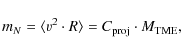
which is proportional to
|
(2) |
the expression for the remaining (N-1) GCs. This procedure is repeated and, in the right panel of Fig. 10, we plot the magnitude of the derivative of mN with respect to n, the number of eliminated GCs.
Obviously, selectively culling the high
relative velocities at large distances drastically lowers the estimate
for the total mass, resulting in large values of
![]() .
Once the algorithm with increasing n starts
removing objects from the overall velocity field, the mass difference
between steps becomes smaller.
.
Once the algorithm with increasing n starts
removing objects from the overall velocity field, the mass difference
between steps becomes smaller.
As can be seen from the right panel of Fig. 10, a convergence is reached after removing four GCs from the red subsample RII. For the blue GCs (BII), the situation is not as clear, and we decide to remove six GCs. For the bright GCs, we remove three GCs.
As opposed to
the constant velocity cuts (at
![]() and
and
![]() )
used in Paper I, this algorithm does not
introduce a de facto upper limit on line-of-sight velocity
dispersion.
)
used in Paper I, this algorithm does not
introduce a de facto upper limit on line-of-sight velocity
dispersion.
Compared to schemes which use a jackknife to search
for ![]() deviations in a local (
deviations in a local (![]() 15
neighbours) velocity
field (which may be ill-defined in the sparsely sampled outer
regions), our approach also works when the rejected GC is not the only
deviant data point in its neighbourhood.
15
neighbours) velocity
field (which may be ill-defined in the sparsely sampled outer
regions), our approach also works when the rejected GC is not the only
deviant data point in its neighbourhood.
5.4 Defining the subsamples
To assess the impact of the interloper removal discussed in the preceding sections, we assign the following labels: the primary label indicates the parent sample (All, BRight, Faint, Blue, and Red, cf. Sect. 5.1), and the Roman numerals I-IV refer to the sequence of interloper removal applied:
- I:
- full data set, no interloper removal;
- II:
- GCs within 3
 of NGC 1404 removed (Sect. 5.2);
- III:
- extreme velocities removed via TME algorithm (Sect. 5.3);
- IV:
- restriction to Class A velocity measurements.
The basic statistical properties of the samples defined above are listed in Table 3 and discussed in the following section.
6 The line-of-sight velocity distribution
We expect the line-of-sight velocity distribution (LOSVD) to be nearly Gaussian. Deviations from Gaussianity may be caused by orbital anisotropies, the presence of interlopers, strong variations of the velocity dispersion profiles with radius, or rotation. Our sample, being the largest of its kind so far, allows us to test the statistical properties of the LOSVD in detail.
Table 3
summarises the statistical properties of the
velocity samples defined in Sect. 5.4.
Besides the
first four moments of the distributions (i.e. mean,
dispersion,
skewness, and kurtosis), we list the p-values
returned by the
Anderson-Darling (AD) and Kolmogorov-Smirnov (KS), and the
Shapiro-Wilks (SW) tests for normality. With the exception of the
dispersion which we
calculate using the expressions given in Pryor
& Meylan (1993), the data listed
in Table 3
were obtained using the functions of the
e1071 and nortest packages
in R-statistics
software![]() for the higher moments and
the normality tests, respectively.
for the higher moments and
the normality tests, respectively.
![\begin{figure}
\par {\includegraphics[width=7.6cm,clip]{12482f19.eps} }\end{figure}](/articles/aa/full_html/2010/05/aa12482-09/img186.png)
|
Figure 11:
Velocity histograms. a): the unfilled histogram
shows all 693 GCs (AI). The solid
histogram bars are the
faint (mR>21.1)
GCs outside the 3 |
| Open with DEXTER | |
The SW test
(Royston
1982; Shapiro
& Wilk 1965) is one of the most popular tests for
normality which also works for small samples. The Anderson-Darling
(Stephens 1974) test is a
variant of the KS-test tailored to be
more sensitive in the wings of the distribution. The SW and
AD tests are among the tests recommended by D'Agostino
& Stephens (1986); note
that these authors caution against the use of the KS test which has a
much smaller statistical power. A detailed
discussion of the application of the AD test in the context of galaxy
group dynamics is given in Hou
et al. (2009). These authors compare the
performance of the AD test to the more commonly used KS and ![]() tests and
find that the AD test is the most powerful of the
three. They conclude that it is a suitable statistical tool to detect
departures from normality, which allows the identification of
dynamically
complex systems.
tests and
find that the AD test is the most powerful of the
three. They conclude that it is a suitable statistical tool to detect
departures from normality, which allows the identification of
dynamically
complex systems.
The velocity histograms for
the entire, the ``bright'', the red and the blue sample are shown in
Fig. 11.
In all four sub-panels, we plot the
corresponding samples prior to any interloper removal (unfilled
histograms). The solid histogram bars show the data after removing
GCs in the vicinity of NGC 1404 and the GCs identified by the
![]() -algorithm (in panel a,
the solid histogram
also excludes the bright GCs). The dashed bars show these
samples when restricted to ``Class A'' velocity measurements.
The
striking difference between the velocity distributions of red and blue
GCs is that the red GCs seem to be well represented by a Gaussian
while the blue GCs appear to avoid the systemic velocity. Also the
distribution of the bright GCs seems to be double-peaked.
-algorithm (in panel a,
the solid histogram
also excludes the bright GCs). The dashed bars show these
samples when restricted to ``Class A'' velocity measurements.
The
striking difference between the velocity distributions of red and blue
GCs is that the red GCs seem to be well represented by a Gaussian
while the blue GCs appear to avoid the systemic velocity. Also the
distribution of the bright GCs seems to be double-peaked.
Below we examine whether these distributions are consistent with being Gaussian.
6.1 Tests for normality
Adopting ![]() as criterion for rejecting the Null hypothesis of
normality, we find that none of the bright
subsamples
(BRI-BRIV) is
consistent with being drawn from a normal
distribution.
as criterion for rejecting the Null hypothesis of
normality, we find that none of the bright
subsamples
(BRI-BRIV) is
consistent with being drawn from a normal
distribution.
The fact that the full sample (AI, AII,
AV) deviates from
Gaussianity (at the ![]() 90
per level) appears to be due to the
presence of the bright GCs: the velocity distribution of objects
fainter than
90
per level) appears to be due to the
presence of the bright GCs: the velocity distribution of objects
fainter than ![]() (sample FII is the union of BII
and RII) cannot be distinguished from a
Gaussian.
(sample FII is the union of BII
and RII) cannot be distinguished from a
Gaussian.
For the red subsamples (RI through RIV), a Gaussian seems to be a valid description. Only the ``extended'' sample (RV) performs worse (probably because it encompasses bright GCs), where the hypothesis of normality is rejected at the 91% level by the KS-test.
While the full blue data set and the sample after removing the GCs near NGC 1404 (BI and BII) are consistent with being Gaussian, the outlier rejection (BIII) and restriction to the ``Class A'' velocities (BIV) lead to significantly lower p-values. In the case of the latter, all tests rule out a normal distribution at the 90% level, which appears reasonable given that the distribution has a pronounced dip (cf. Fig. 11, panel (c), dashed histogram).
Below we address in more detail the deviations from Gaussianity, as quantified by the higher moments of the LOSVD.
6.2 Moments of the LOSVD
6.2.1 Mean
Assuming that the GCs are bound to NGC 1399, the first moment
of the
LOSVD is expected to coincide with the systemic velocity of the
galaxy, which is
![]() (Paper I).
As can be
seen from the third column in Table 3, this is,
within
the uncertainties, the case for all subsamples, with the exception of
R I, where the GCs in the vicinity of
NGC 1404 are responsible
for increasing the mean velocity.
(Paper I).
As can be
seen from the third column in Table 3, this is,
within
the uncertainties, the case for all subsamples, with the exception of
R I, where the GCs in the vicinity of
NGC 1404 are responsible
for increasing the mean velocity.
6.2.2 Dispersion
The second moments (Table 3,
Col. 5), the dispersions,
are calculated using the maximum-likelihood method presented by
Pryor & Meylan (1993),
where the individual velocities are weighted by their
respective uncertainties. Note that these estimates do not differ from
the standard deviations
given in Col. 4 by more than
![]() .
The interloper
removal, by construction, lowers the velocity dispersion. The largest
decrease can be found for the blue GCs, where the difference between
B I and B III
is
.
The interloper
removal, by construction, lowers the velocity dispersion. The largest
decrease can be found for the blue GCs, where the difference between
B I and B III
is ![]() .
For the red sample,
the corresponding value is
.
For the red sample,
the corresponding value is
![]() .
We only consider at
this stage the full radial range of the sample. As will
be shown later, the effect of the interloper removal on the dispersion
calculated for individual radial bins can be much larger.
.
We only consider at
this stage the full radial range of the sample. As will
be shown later, the effect of the interloper removal on the dispersion
calculated for individual radial bins can be much larger.
The
main feature is that the dispersions for the blue and red GCs differ
significantly, with values of ![]() and
and
![]() for
the blue and red samples
(BIII and RIII),
respectively. The corresponding
values given in Paper I (Table 2) are
for
the blue and red samples
(BIII and RIII),
respectively. The corresponding
values given in Paper I (Table 2) are
![]() and
and
![]() .
The agreement for the red GCs is good, and the discrepancy found for
the blue GCs is due to the different ways of treating extreme
velocities: in Paper I such objects were culled from the
sample by
imposing radially constant velocity cuts (at 800 and
.
The agreement for the red GCs is good, and the discrepancy found for
the blue GCs is due to the different ways of treating extreme
velocities: in Paper I such objects were culled from the
sample by
imposing radially constant velocity cuts (at 800 and
![]() ),
while the method employed here (see
Sect. 5.3)
does not operate with fixed upper/lower
limits, which leads to a larger dispersion.
),
while the method employed here (see
Sect. 5.3)
does not operate with fixed upper/lower
limits, which leads to a larger dispersion.
6.2.3 Skewness
Coming back to the issue of Gaussianity, we calculate the third moment
of the LOSVD: the skewness is a measure of the symmetry of a
distribution (the Gaussian, being symmetric with respect to the mean,
has a skewness of zero):
![\begin{displaymath}{\rm {skew}}= \frac{1}{N} \sum_{j=1}^{N} \left[ \frac{x_j -
\bar{x}}{\sigma} \right]^3 \cdot
\end{displaymath}](/articles/aa/full_html/2010/05/aa12482-09/img197.png)
|
(3) |
The uncertainties were estimated using a bootstrap (with 999 resamplings). We consistently find a negative skewness for the bright subsamples (BRI-BRIV, Fig. 11b), i.e. there are more data points in the low-velocity tail of the distribution.
The blue GCs also show a negative skewness, which is significant for the samples BIII and BIV (cf. Fig. 11c). A similar finding was already described in Paper I.
The distribution of the red GCs is symmetric with respect to the systemic velocity, as is to be expected for a Gaussian distribution (cf. Fig. 11d).
6.2.4 Kurtosis
In the following, ![]() denotes the reduced kurtosis, or
kurtosis excess (to assign the value zero to a
normal
distribution), i.e.:
denotes the reduced kurtosis, or
kurtosis excess (to assign the value zero to a
normal
distribution), i.e.:
![\begin{displaymath}\kappa = \frac{1}{N} \sum_{j=1}^{N} \left[ \frac{x_j -
\bar{x}}{\sigma} \right]^4 - 3 ~.
\end{displaymath}](/articles/aa/full_html/2010/05/aa12482-09/img198.png)
|
(4) |
The reduced kurtosis
The blue samples (BI-BIV), on the other hand, have a negative kurtosis, indicative of a more flat-topped distribution which might be the result of a tangential orbital bias.
The red GCs are
consistent with ![]() ,
which would be expected in the case of
isotropic orbits.
,
which would be expected in the case of
isotropic orbits.
6.3 Summary of the statistical tests
We briefly summarise the main findings from the above statistical considerations. The velocity dispersions of the red and blue subsamples are, as in Paper I, significantly different, with the blue GCs showing a larger dispersion. We note that the dispersions of the bright (mR < 21.1) subsamples have values in between those found for the red and blue GCs.
The entirety of the GCs (AI, AII) is not Gaussian, which is most likely due to the pronounced skewness of the brightest GCs.
The blue subsamples, although formally consistent with being Gaussian, show (after the outlier rejection) significantly negative values for both skewness and kurtosis.
The red GCs are well represented by a Gaussian, which would be expected in the case of isotropic orbits.
7 Rotation
The amount of rotation found in a GCS and among its subpopulations might be indicative of the host galaxy merger history. The presence of rotation (rather than the absence thereof, since one only observes projected rotation), might help constrain GCS formation scenarios.
![\begin{figure}
\par {\includegraphics[width=8cm,clip]{12482f20.eps} }\end{figure}](/articles/aa/full_html/2010/05/aa12482-09/img203.png)
|
Figure 12:
Rotation of the NGC 1399 GCS. Velocities versus position
angle. The upper panel shows the data for the
blue sample
BIII (i.e. the data after the removal of the
GCs in the
vicinity of NGC 1404 and the outlier rejection) for the
azimuthally
complete radial interval
|
| Open with DEXTER | |
In Paper I, we did not find any signature of rotation, with
the
exception of the outer (
![]() )
metal-poor
GCs, for which a marginal rotation amplitude of
)
metal-poor
GCs, for which a marginal rotation amplitude of
![]() was
detected (for a position angle of
was
detected (for a position angle of
![]() ).
Our revised and extended
data set provides the opportunity to re-examine this finding.
).
Our revised and extended
data set provides the opportunity to re-examine this finding.
We apply the method used in Paper I, which consists
of fitting a
sine-curve to the velocities plotted versus the position angle (as
shown in Fig. 12):
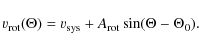
Further, to ensure that the rotation signal is not merely an artifact of the inhomogeneous spatial and azimuthal coverage, we calculate the rotation amplitude for 1000 Monte Carlo (MC) realizations, in which we keep the positions of our original dataset but permutate the velocities. From this we determine the fraction f of MC runs for which a rotation amplitude larger than the observed one was found: i.e. the smaller the value of f, the higher the significance of the rotation signal.
Table 4
lists the values
for various GC subsamples. Since, as can be seen from
Fig. 7
(bottom right panel), the azimuthal coverage
becomes very patchy for galactocentric distances beyond about
![]()
![]() ,
we also give the results for
the radial range
,
we also give the results for
the radial range
![]() ,
where the spatial
coverage is more uniform and the completeness
(cf. Fig. 7,
bottom left panel) is relatively
high. This selection is then further divided into an ``inner''
(
,
where the spatial
coverage is more uniform and the completeness
(cf. Fig. 7,
bottom left panel) is relatively
high. This selection is then further divided into an ``inner''
(
![]() )
and an ``outer''
(
)
and an ``outer''
(
![]() )
region.
)
region.
Table 4: Rotation amplitudes and angles for the different subsamples.
7.1 Rotation of the brightest GCs
The brightest GCs ( mR < 21.1), show no sign of rotation. For all selections (BRI-BRIV) and radial intervals considered in Table 4, the rotation amplitude is consistent with being zero.
7.2 Rotation of the metal-rich GCs
For the metal-rich GCs, only the sample RIII
(i.e. the data set obtained after
masking the GCs in the vicinity of NGC 1404 and applying the
outlier
rejection algorithm) shows a weak rotation signal
(
![]() )
for the
``outer sample''. The data and the fit are shown in the lower panel of
Fig. 12.
The corresponding f-value of 0.27 shows
that a rotation signal of this magnitude arises from the randomised
data with a probability of 27 per cent, meaning no significant
rotation is detected for the red GCs. Moreover, this weak rotation
signal vanishes completely when only the ``Class A'' velocity
measurements are considered (RIV).
)
for the
``outer sample''. The data and the fit are shown in the lower panel of
Fig. 12.
The corresponding f-value of 0.27 shows
that a rotation signal of this magnitude arises from the randomised
data with a probability of 27 per cent, meaning no significant
rotation is detected for the red GCs. Moreover, this weak rotation
signal vanishes completely when only the ``Class A'' velocity
measurements are considered (RIV).
7.3 Rotation of the metal-poor GCs
Within the central
![]()
![]() ,
none of the blue
GC subsamples shows any rotation signal. For the ``outer samples'',
however, the rotation amplitudes lie in the range
110-126
,
none of the blue
GC subsamples shows any rotation signal. For the ``outer samples'',
however, the rotation amplitudes lie in the range
110-126
![]() ,
and the values obtained for
,
and the values obtained for
![]() agree within
the uncertainties. For the blue GCs
BII (after removal of GCs near
NGC 1404), the amplitude is
agree within
the uncertainties. For the blue GCs
BII (after removal of GCs near
NGC 1404), the amplitude is
![]() ,
and
,
and ![]() (see
Fig. 12,
upper panel), which agrees with the rotation
values quoted in Paper I. After further restricting this
sample to ``Class A''
velocities, the results agree very well, although the smaller number
of data points leads to larger uncertainties. We
caution, however, that the probability of such an amplitude resulting
from the randomised data still is
about 10 per cent.
(see
Fig. 12,
upper panel), which agrees with the rotation
values quoted in Paper I. After further restricting this
sample to ``Class A''
velocities, the results agree very well, although the smaller number
of data points leads to larger uncertainties. We
caution, however, that the probability of such an amplitude resulting
from the randomised data still is
about 10 per cent.
7.4 NGC 1399 and the rotation of its GCS
As stated above, we find no rotation for the red (metal-rich)
GC population. In this respect, the red GCs appear to reflect
the
properties of the stellar body of NGC 1399 for which the
spectroscopic study by Saglia
et al. (2000) found only a small (![]()
![]() )
rotation along the major axis (an equally small
signal was found for the slightly off-centre slit position parallel
to the minor axis).
)
rotation along the major axis (an equally small
signal was found for the slightly off-centre slit position parallel
to the minor axis).
For the blue GCs, a significant rotation
signature is found for the radial range between 4 and 8
arcminutes. The axis of rotation is consistent with the photometric
major axis of NGC 1399 (
![]() ). Due to the very patchy
angular coverage for radii beyond about 8
). Due to the very patchy
angular coverage for radii beyond about 8![]() ,
no statement about
the rotation of the GCs beyond
,
no statement about
the rotation of the GCs beyond ![]()
![]() can be made.
can be made.
In
the literature the amount of rotation is quantified in terms of the
parameter
![]() ,
(i.e. the
ratio of rotational velocity to velocity dispersion). For
NGC 1399
we find
,
(i.e. the
ratio of rotational velocity to velocity dispersion). For
NGC 1399
we find ![]() for the metal-rich GCs and
for the metal-rich GCs and
![]() for
the metal-poor GCs.
for
the metal-poor GCs.
8 Radial velocity dispersion profiles
The line-of-sight velocity dispersion as a function of the projected radius is the quantity we aim to reproduce with the Jeans models described in Sect. 9. The histograms displayed in Fig. 11 and the data given in Table 3 show that the blue and red subpopulations have significantly different velocity distributions, as is already known from Paper I. We calculate the dispersion profiles separately for both subpopulations. First, we determine the dispersion values using the same annular bins for both subpopulations and divide our data into radial bins covering the full radial range (starting at 1.0,3.5,5.5,7.5,9.5,12.5,15.5, and 30.0 arcmin). The limits of the bins are shown as dotted lines in the upper and middle panels of Fig. 13.
The middle panels of Fig. 13 show the radial dispersion profiles for the red and blue GCs. Circles show the values obtained for the GCs fainter than mR=21.1, prior to any interloper removal (samples RI and BI for red and blue GCs, respectively). The corresponding profiles obtained after removing the GCs in the vicinity of NGC 1404 and the most extreme velocities (samples RIII and BIII) are shown as filled squares. For the extended samples RV and BV, shown as diamonds, the number of GCs in a bin is given in parenthesis. The dispersion profiles for the fixed radial bins for the samples RI through RV and BI-BV are given in Table A.1.
Next, to obtain data points with similar statistical uncertainties, we fix the number of GCs per bin (and thereby allow for a larger range in radial extent of the bins). In the bottom panels of Fig. 13, we use a moving window containing 35 GCs to plot the samples RIII and BIII together with the extended samples containing the B+07 measurements RV and BV. The corresponding values are listed in Table A.2.
![\begin{figure}
\par\includegraphics[width=14cm,clip]{12482f21.eps}
\end{figure}](/articles/aa/full_html/2010/05/aa12482-09/img234.png)
|
Figure 13: Velocity diagrams and line-of-sight velocity dispersion profiles. Upper left: radial velocity vs. galactocentric distance for the red GCs. Dots and circles show faint and bright ( mR < 21.1 mag) GCs, respectively. Large and small triangles are the data points from Bergond et al. (2007) with Class A and B velocity measurements, respectively (see text for details). Squares mark GCs rejected on account of their proximity to NGC 1404; crosses are the GCs removed by the TME rejection algorithm. The solid and dashed horizontal lines are the systemic velocities of NGC 1399 and NGC 1404, respectively. The vertical dashed line shows the (projected) distance of NGC 1404. The dotted vertical lines show the radial bins for which the dispersion shown in the middle panels is calculated. Upper right: the same for the blue GCs. Middle panels: the dispersion profiles for fixed radial bins. Circles are the values obtained for the full samples (RI and BI) prior to any interloper removal. Filled squares show the values after removing GCs in the vicinity of NGC 1404 and the outliers identified by the TME algorithm (samples RIII and BIII). The dispersion profiles for the extended samples (RV and BV) including the velocities from Bergond et al. (2007) are shown as diamonds. The labels in parentheses give the number of GCs in a given bin. Bottom panels: filled squares are the profiles for RIII and BIII obtained for a moving bin comprising 35 GCs. Diamonds show the same for the samples RV and BV. These moving-bin profiles which are used for the modelling in Sect. 10 are listed in Table A.2. |
| Open with DEXTER | |
8.1 Dispersion of the metal-rich subpopulation
For RIII and RV,
shown in the middle left panel of
Fig. 13,
we find that the velocity dispersion
declines for radii beyond ![]()
![]() ,
while the values for
the sample RI (prior to any interloper
rejection) even show
an increasing dispersion. The removal of the GCs in the vicinity of
NGC 1404 mostly affects the 4th bin where the
dispersion
drops from
,
while the values for
the sample RI (prior to any interloper
rejection) even show
an increasing dispersion. The removal of the GCs in the vicinity of
NGC 1404 mostly affects the 4th bin where the
dispersion
drops from ![]() to
to ![]() .
Removing the
three potential outliers in the 5th bin by means of the
TME-algorithm lowers the dispersion by about
.
Removing the
three potential outliers in the 5th bin by means of the
TME-algorithm lowers the dispersion by about
![]() .
.
The bottom left panel of
Fig. 13
compares the moving-bin results for the
samples RIII and RV.
Both samples show again a
smooth decline of the dispersion for larger radii. The marginally
higher values found for the RV data which
include the B+07
velocities is likely due to the inclusion of brighter (
![]() )
clusters which have a higher velocity dispersion than
the fainter red GCs. The 3rd bin for RIII
has a
surprisingly high dispersion of
)
clusters which have a higher velocity dispersion than
the fainter red GCs. The 3rd bin for RIII
has a
surprisingly high dispersion of
![]() which
is
50 (67)
which
is
50 (67) ![]() higher than the value found in the previous
(next) bin. This rise is caused by a number of GCs at high velocities
(cf. Fig. 9),
leading to a mean velocity which
exceeds the systemic velocity of NGC 1399 by
higher than the value found in the previous
(next) bin. This rise is caused by a number of GCs at high velocities
(cf. Fig. 9),
leading to a mean velocity which
exceeds the systemic velocity of NGC 1399 by
![]()
![]() .
In the upper panel of
Fig. 14,
where we show the dispersion in a
semi-logarithmic plot, the deviation of this data point becomes even
more evident. In the modelling presented in
Sect. 10
this data point (marked by an asterisk in
Table A.2)
is omitted.
.
In the upper panel of
Fig. 14,
where we show the dispersion in a
semi-logarithmic plot, the deviation of this data point becomes even
more evident. In the modelling presented in
Sect. 10
this data point (marked by an asterisk in
Table A.2)
is omitted.
8.2 Dispersion of the metal-poor subpopulation
For the blue GCs (shown in the right panels of
Fig. 13)
the situation is more complicated in so far as the dispersion profile
is not as smooth. For the full sample
BI as shown in the middle right panel of
Fig. 13,
the dispersion rises quite sharply by over
![]() for
the range between
for
the range between ![]() 10
and
10
and
![]() where it reaches almost
where it reaches almost
![]() before
levelling out at
before
levelling out at ![]()
![]() .
The effect of the
interloper removal is strongest for the fifth bin where removing five
GCs (four of which are in the vicinity of NGC 1404 and one GC
is
rejected by the TME algorithm, sample BIII)
decreases the
dispersion by more than
.
The effect of the
interloper removal is strongest for the fifth bin where removing five
GCs (four of which are in the vicinity of NGC 1404 and one GC
is
rejected by the TME algorithm, sample BIII)
decreases the
dispersion by more than
![]() .
For the sixth bin,
however, the dispersion is again somewhat higher (although the values
agree within the uncertainties). For the sample BI
and
BIII no clear trend for the behaviour of the
GCs towards
larger radii is discernible.
.
For the sixth bin,
however, the dispersion is again somewhat higher (although the values
agree within the uncertainties). For the sample BI
and
BIII no clear trend for the behaviour of the
GCs towards
larger radii is discernible.
Taking into account the velocities for the outer GCs by B+07 shows however, that also the blue GCs have a declining velocity dispersion profile (sample BV, shown as diamonds).
The lower right panel of Fig. 13 shows the velocity dispersion profiles for the samples BIII and BV for a moving window containing 35 GCs. Compared to the red GCs these profiles appear less continuous. This behaviour is likely due to inhomogeneities and substructures in the velocity field as illustrated in the right panel of Fig. 9.
8.3 Comparison to the stellar data
In Fig. 14
we compare our values to the results
presented by Saglia et al.
(2000). These authors used
Gauss-Hermite polynomials to analyse absorption-line spectra of the
stellar body of NGC 1399 out to
![]() (
(![]()
![]() .
The radial ranges covered by both data sets only have a marginal
overlap.
.
The radial ranges covered by both data sets only have a marginal
overlap.
Stellar velocity dispersion profile:
in the upper panel of Fig. 14 we plot the velocity dispersion profiles for the blue and red GCs (BIII, RIII) obtained for moving bins of 35 GCs (same as the bottom panels in Fig. 13). With the exception of the third data point, the red GCs appear to follow the trend shown by the stars in NGC 1399. Only the innermost blue data point is comparable to the stellar data, all subsequent bins show a much higher dispersion.The fourth moment:
in the lower panel of Fig. 14 we compare Gauss-Hermite h4 values given by Saglia et al. to the corresponding values for the GCs which were converted from the
We find that the value for the blue GCs (sample BIII) lies significantly below the stellar values, while the value for the red GCs (RIII) seems to agree with the h4 values of the stars. This figure also demonstrates that
![\begin{figure}
\par {\includegraphics[width=7.8cm,clip]{12482f22.eps} }
\par\vspace*{2mm}
{\includegraphics[width=7.8cm,clip]{12482f23.eps} }\end{figure}](/articles/aa/full_html/2010/05/aa12482-09/img248.png)
|
Figure 14: Comparison to the stellar kinematics presented by Saglia et al. (2000). Upper panel: line-of-sight velocity dispersion profiles. Diamonds show the stellar kinematics, dots and crosses are our measurements of the red (R III) and blue (B III) GCs, respectively. Lower panel: Gauss-Hermite parameter h4 (Eq. (6)) vs. projected radius. The values for the blue and red GCs are shown as long-dashed and dashed rectangle, respectively. The solid grey rectangle shows the value for the combined red and blue sample. The values derived from absorption-line spectroscopy by Saglia et al. (2000) are shown as diamonds, and the dashed line represents their best fit model (cf. their Fig. 5). |
| Open with DEXTER | |
9 Jeans models
The mass profile of NGC 1399 is estimated by comparing the values derived from spherical, non-rotating Jeans models to the observed line-of-sight velocity dispersions. The assumption of spherical symmetry is justified by the near-spherical appearance of the galaxy. To account for the degeneracy between mass and orbital anisotropy, which can only be broken using much larger datasets than ours, we calculate models for different (constant) values of the anisotropy parameter9.1 The Jeans equation
The spherical, non-rotating Jeans equation reads:
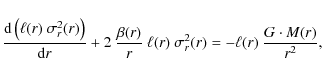
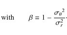
Here, r is the true 3D radial distance from the centre and
For our
analysis, we use the expressions given by e.g. Mamon & okas (2005),
see also van der Marel
& Franx (1993). Given a mass distribution M(r),
a
three-dimensional number density of a tracer population ![]() ,
and a constant anisotropy parameter
,
and a constant anisotropy parameter ![]() ,
the solution to
the Jeans equation (Eq. (7))
reads:
,
the solution to
the Jeans equation (Eq. (7))
reads:
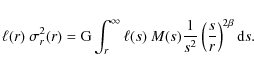
This expression is then projected using the following integral:
![\begin{displaymath}\sigma_{{\rm los}}^{2}(R)= \frac{2}{N(R)} \left[ \int_{R}^{\i...
...\ell \sigma_{r}^{2}~ {\rm d}r}{r \sqrt{r^{2}-R^{2}}} \right]~,
\end{displaymath}](/articles/aa/full_html/2010/05/aa12482-09/img256.png)
where N(R) is the projected number density of the tracer population, and
9.2 Globular cluster number density profiles
Table 5: Globular cluster number density profiles.
The GCS of NGC 1399 has been the target of two wide-field photometric studies. The work presented by (Bassino et al. 2006, hereafter B+06) extends the earlier D+03 study upon which the analysis presented in Paper I was based. For our analysis, we use a cored power-law profile (Reynolds-Hubble law) to fit the data from B+06: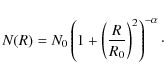
Here, R0 is the core radius, and
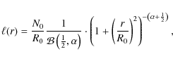
where
Figure 15
shows the number density
profiles for the blue (open squares) and red GCs (circles) as given in
B+06, together with the corresponding fits. One clearly sees that the
red GCs have a steeper number density profile than the blue
GCs. For reference, the surface brightness profile of NGC 1399
(as given by D+03, but scaled to match the red GC profile) is shown
with diamonds. Note that in the region of overlap (
![]() )
the slope of the densities of the stars and
the red GCs are indistinguishable.
)
the slope of the densities of the stars and
the red GCs are indistinguishable.
![\begin{figure}
\par {\includegraphics[width=7.8cm,clip]{12482f24.eps} }\end{figure}](/articles/aa/full_html/2010/05/aa12482-09/img268.png)
|
Figure 15: GC number density profiles. The data from B+06 are shown together with the fits to Eq. (10). Circles and squares represent the red and blue GCs, respectively. The fits to the red and the blue number density distributions are shown as dashed and solid line, respectively. The coefficients are listed in Table 5. The dashed and solid arrows indicate the core radii R0 as returned from the fits for the red and blue GCs, respectively. Diamonds show the surface brightness profile of NGC 1399, as given in Table 4 of D+03 (the data points have been shifted for comparison with the red GC number density profile). |
| Open with DEXTER | |
9.3 Luminous matter
In order to assess the dark matter content of NGC 1399, we first need a model for the luminous matter. Moreover, the spatial distribution of the stars is needed to model the stellar velocity dispersion profile (see Sect. 10.4.2).
9.3.1 Deprojection of the surface brightness profile
D+03 give the following fit to the R-band surface
brightness profile
of NGC 1399:
![\begin{displaymath}\mu(R)= 2.125 \log \left[ 1+ \left(\frac{R}{0\hbox{$.\mkern-4mu^\prime$ }055}
\right)^2\right] + 15.75 ,
\end{displaymath}](/articles/aa/full_html/2010/05/aa12482-09/img269.png)
where R is the projected radius. Assuming an absolute solar luminosity of
![\begin{displaymath}I(R) = 1.10\times 10^4 \left[1+ \left( \frac{R}{0\hbox{$.\mkern-4mu^\prime$ }055}\right)^2
\right]^{-0.85} .
\end{displaymath}](/articles/aa/full_html/2010/05/aa12482-09/img272.png)
At a distance of 19 Mpc,
![\begin{displaymath}j(r)\left[ \frac{L_{\odot}}{\rm {pc}^{3}} \right] = 16.33 \le...
... \left( \frac{r}{304~\rm {pc}}\right)^2
\right]^{-1.35} \cdot
\end{displaymath}](/articles/aa/full_html/2010/05/aa12482-09/img276.png)
We now compare this to the deprojected profile given in D+03. These authors obtained the three-dimensional luminosity distribution by numerically projecting a cored power-law and compare the result to the fitted surface brightness profile. The luminosity density profile they obtained using this procedure reads:
![\begin{displaymath}L_{\rm {T_1}}\left[ \frac{L_{\odot}}{\rm {pc}^{3}} \right]= 101 \left[ 1+ \frac{r}{221~\rm {pc}} \right]^{-2.85} \cdot
\end{displaymath}](/articles/aa/full_html/2010/05/aa12482-09/img277.png)
One notes that the central luminosity density of this profile is more than six times higher than what we find in Eq. (14). Further, the profile presented by D+03 is slightly steeper.
To show the difference between the two deprojections, we plot in Fig. 16 the surface brightness profile of NGC 1399 as given in Table 4 of D+03, together with the fit (Eq. (12), solid line) and the re-projection of their luminosity density profile (dashed line). The latter overestimates the measured surface brightness of NGC 1399 and therefore results in a larger stellar mass.
![\begin{figure}
\par {\includegraphics[width=8.4cm,clip]{12482f25.eps} }\end{figure}](/articles/aa/full_html/2010/05/aa12482-09/img278.png)
|
Figure 16: Comparison between different deprojections of the surface brightness profile of NGC 1399: the dashed curve is the re-projection of the luminosity density profile as given in D+03 (Eq. (15)). The solid curve shows the fit to the data (Eq. (12)), which corresponds to there-projection of Eq. (14). |
| Open with DEXTER | |
9.3.2 Stellar mass-to-light ratio
In Paper I, Richtler et al. quote an R-band
stellar
mass-to-light ratio of M/LR=5.5,
which they obtained by
converting the B-band value derived by Saglia et al. (2000).
Recently,
Gebhardt et al. (2007)
used the Hubble Space Telescope to
obtain kinematics for the very central part of NGC 1399 in
order to
measure the mass of the nuclear black hole. From their dynamical
models, these authors find a best-fit
![]() for
a
distance of
for
a
distance of
![]() .
At a distance of
.
At a distance of ![]() ,
as
assumed in this study, this corresponds to
,
as
assumed in this study, this corresponds to
![]() ,
which
is in excellent agreement with the value given in Paper I. We
thus
adopt a stellar mass-to-light ratio of
,
which
is in excellent agreement with the value given in Paper I. We
thus
adopt a stellar mass-to-light ratio of
![]() .
.
9.3.3 Enclosed stellar mass
We obtain the enclosed stellar mass by integrating Eq. (14):
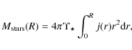
|
(16) |
which can be expressed in terms of the hypergeometric function:
![\begin{displaymath}M(R) = C_1 \cdot \frac{3}{4} \pi \Upsilon_{\star}~ R^3
~_{2}...
...a \right],\left[ \frac{5}{2}\right],
-\frac{R^2}{B^2} \right),
\end{displaymath}](/articles/aa/full_html/2010/05/aa12482-09/img285.png)
where C1=16.33 is the constant,
In practice, the
hypergeometic function can be calculated to arbitrary precision
(e.g. Press et al. 1992),
but the computation of the integral
over M(R) becomes very
time-consuming. In the programme calculating
the Jeans-models, we therefore apply a piece-wise definition of the
mass profile, using only standard functions: for radii smaller than
3430 pc, we use a 6th-order polynomial, and a
3rd-order polynomial in the range
![]() .
For
.
For ![]() the following expression is a good
approximation to Eq. (17):
the following expression is a good
approximation to Eq. (17):
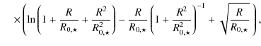
|
(18) |
where
9.5 The
anisotropy parameter 
The solutions to the Jeans equation given in Eq. (8) are
defined for constant values of the anisotropy
parameter. Since ![]() cannot
be determined from the data itself, we calculate our models for
a set of anisotropy parameters. The higher moments derived in
Sect. 8.3
suggest that the red cluster population is most
likely isotropic, possibly slightly radial, while the blue GCs might
show a mild tangential bias. We therefore use
cannot
be determined from the data itself, we calculate our models for
a set of anisotropy parameters. The higher moments derived in
Sect. 8.3
suggest that the red cluster population is most
likely isotropic, possibly slightly radial, while the blue GCs might
show a mild tangential bias. We therefore use
![]() for
modelling the GCs.
for
modelling the GCs.
9.5 Dark matter profiles
Numerical cosmological simulations predict cuspy dark matter density
profiles (e.g. Bullock
et al. 2001). However, the very
inner shape apparently depends on numerical details (e.g. Diemand et al. 2005),
while agreement is reached regarding the outer
profile which declines as R-3.
Here we use an NFW (Navarro
et al. 1997) halo to represent a cuspy dark
component. The
density profile is given by:
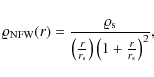
and the cumulative mass reads:
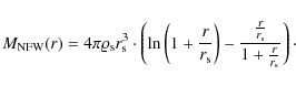
However, in low surface brightness galaxies, where dark matter contributes significantly already in the central regions, most observations are not compatible with a cuspy halo (Gentile et al. 2007) but rather with a cored density profile. We therefore also model a dark matter density profile with a core. One possibility is to use the density profile, which Burkert (1995) introduced to represent the dark matter halo of dwarf galaxies. For this halo, the density profile is:
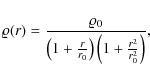
and the cumulative mass is given by the following expression:
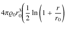
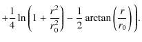
10 Mass models for NGC 1399
In this section, we present the results of the Jeans modelling. First, we treat the tracer populations separately, i.e. we fit the velocity dispersion profiles of the red and blue GC samples using NFW halos. In a second step, we search for a set of parameters to describe both populations. The stellar velocity dispersion profile by Saglia et al. (2000) is then used to put further constraints on the mass model of NGC 1399. Finally, the results for the NFW halos are compared to cored Burkert halo models.
10.1 Jeans analysis
To obtain an estimate for the NGC 1399 mass profile, we
compare the
observed velocity dispersion profiles to Jeans models
(Eq. (9)).
The stellar mass-to-light ratio is assumed to be constant (see
Sect. 9.3),
and the (constant) anisotropy parameter
takes the values ![]() ,
or +0.5 (corresponding to a mild
tangential, isotropic, and a slightly radial orbital bias). To find
the best Jeans model, we adjust the parameters of the dark halo.
,
or +0.5 (corresponding to a mild
tangential, isotropic, and a slightly radial orbital bias). To find
the best Jeans model, we adjust the parameters of the dark halo.
The dark matter halos considered here (NFW and Burkert halos)
are
characterised by two parameters, a scale radius
![]() and
a
density
and
a
density ![]() .
For a given tracer population and
anisotropy
.
For a given tracer population and
anisotropy ![]() ,
we calculate a grid of models where the density
acts as free parameter while the radii have discrete values,
i.e.
,
we calculate a grid of models where the density
acts as free parameter while the radii have discrete values,
i.e.
![]() .
The results
of this modelling are summarised in Table 6, which
quotes the best-fit halo parameters and the corresponding
.
The results
of this modelling are summarised in Table 6, which
quotes the best-fit halo parameters and the corresponding ![]() values for
the different tracer populations and anisotropies.
values for
the different tracer populations and anisotropies.
The
confidence level (CL) contours are calculated using the definition by
Avni (1976),
i.e. using the difference
![]() above
the
minimum
above
the
minimum ![]() value. With two free parameters,
e.g.
value. With two free parameters,
e.g.
![]() the
68, 90, and 99 per
cent contours correspond to
the
68, 90, and 99 per
cent contours correspond to
![]() ,
and 9.21,
respectively.
,
and 9.21,
respectively.
To facilitate the comparison of the results for the
NFW halos to values in the literature, we use the equations given in
Bullock et al. (2001)
to express the (
![]() )
pairs in terms
of the virial parameters (
)
pairs in terms
of the virial parameters (
![]() ).
These authors
define the virial radius
).
These authors
define the virial radius ![]() such that the mean density
within this radius is
such that the mean density
within this radius is
![]() times
the mean density
of the universe, and the concentration parameter is defined as
times
the mean density
of the universe, and the concentration parameter is defined as
![]() .
The confidence contours in
Fig. 17
are shown in the
(
.
The confidence contours in
Fig. 17
are shown in the
(
![]() )
parameter space.
)
parameter space.
Table 6: Jeans modelling best fit parameters.
![\begin{figure}
\par\mbox{\includegraphics[width=4cm,clip]{12482f26.eps}\hspace*{...
...s}\hspace*{0.5cm}
\includegraphics[width=4cm,clip]{12482f34.eps} }\end{figure}](/articles/aa/full_html/2010/05/aa12482-09/img328.png)
|
Figure 17:
Mass models (NFW halo): confidence level contours (68%, 90%, and 99%).
The x-axis plots the virial mass (
|
| Open with DEXTER | |
![\begin{figure}
\par\mbox{{\includegraphics[width=4.8cm,clip]{12482f35.eps} }\hsp...
...space*{0.5cm}
{\includegraphics[width=4.8cm,clip]{12482f37.eps} }}\end{figure}](/articles/aa/full_html/2010/05/aa12482-09/img329.png)
|
Figure 18:
Best fit Jeans models (NFW halo). Left panel:
NGC 1399 GC data and modelled velocity dispersion profiles.
Crosses
and dots show the red (RIII) and blue (BIII)
velocity dispersion profiles (for a moving bin of 35 GCs,
cf. Fig. 13,
lower panels), respectively. The
thin curves are the best fit models obtained
for the red
(models a1-a3) and the blue GCs (models a4-a6)
separately. The thick lines (with labels) show
the dispersions
for the combined model for red and blue GCs (models a7
and
a8). Middle panel: the
same for the ``extended'' samples
including the Bergond
et al. (2007) measurements (samples RV
and
BV). Right panel: red
GCs and stars. Diamonds show
the stellar velocity dispersion (Saglia
et al. 2000), the red GCs
(RIII) are shown as dots. The thin lines are
the models for
the individual tracer populations, i.e. models c1
and c2
for the stars and models a1-a3 for the red GCs.
The thick
curves are the joint solutions, i.e. models a9
and a10.
In all panels, solid lines are isotropic models, and the models with
|
| Open with DEXTER | |
One immediately notices that the contours for the GCs (shown in the top and middle row of Fig. 17) are quite elongated, with a negative correlation between the virial mass and concentration. Below we discuss the results obtained for the different tracer populations.
10.2 NFW-models for the metal-rich population
The top row of Fig. 17
shows the NFW model parameters
for the metal-rich (red) GCs. For a given value of ![]() ,
the
halos derived for the sample RIII
(i.e. metal-rich GCs
fainter than mR=21.1,
after removal of GCs in the vicinity of
NGC 1404 and the outlier-rejection as described in
Sect. 5)
are somewhat less massive and less
concentrated than the halos found for the ``extended'' sample
RV. The reason is that the latter includes
bright GCs for
which we found a larger velocity dispersion
(e.g. Fig. 13,
lower left panel). Note however
that the models for RIII and RV
agree within their
respective 90% contours. The results also agree well with the halo
parameters presented in Paper I (shown as a circle in
Fig. 17).
,
the
halos derived for the sample RIII
(i.e. metal-rich GCs
fainter than mR=21.1,
after removal of GCs in the vicinity of
NGC 1404 and the outlier-rejection as described in
Sect. 5)
are somewhat less massive and less
concentrated than the halos found for the ``extended'' sample
RV. The reason is that the latter includes
bright GCs for
which we found a larger velocity dispersion
(e.g. Fig. 13,
lower left panel). Note however
that the models for RIII and RV
agree within their
respective 90% contours. The results also agree well with the halo
parameters presented in Paper I (shown as a circle in
Fig. 17).
The modelled dispersion profiles are
compared to the observational data in the left and middle panel of
Fig. 18.
For both RIII and RV,
the
agreement between models and data is very good, and the best-fit
models (shown as thin lines) for the different values of the
anisotropy parameter ![]() are indistinguishable. The model
parameters listed in Table 6 illustrate the
mass-anisotropy degeneracy, where the virial mass increases with
are indistinguishable. The model
parameters listed in Table 6 illustrate the
mass-anisotropy degeneracy, where the virial mass increases with
![]() .
.
10.3 NFW models for the metal-poor GCs
The shape of the velocity dispersion profiles of the metal-poor GCs
is not as smooth as that of the metal-rich GC population. The ``jumps''
in the profiles may be caused by the presence of interlopers. Since
the dispersion values of adjacent bins show quite strong variations,
the ![]() values derived when modelling the blue GCs are
substantially larger than those found for the red GCs.
values derived when modelling the blue GCs are
substantially larger than those found for the red GCs.
The parameters derived for the sample BIII and the ``extended'' sample BV differ significantly: as can be seen from the middle row in Fig. 17, the solutions for the extended sample (solid contours) have a smaller virial mass and a larger concentration.
Compared to the models for the red GCs, the dark halos derived from the dispersion profile of the blue GCs are up to an order of magnitude more massive and about four times less concentrated which, as will be detailed below, considerably complicates the task of finding a common solution.
10.4 Finding joint solutions
Given that the different tracer populations (i.e. metal-rich and
metal-poor GCs, and stars) move in the same potential, it is necessary
to find a joint solution. For a set of tracer populations (labelled
a and b), we determine the
combined parameters by minimising the
sum ![]() in the
in the
![]() )-parameter
space. Since the
tracer populations may have different orbital anisotropies, this
procedure is performed for different combinations of
)-parameter
space. Since the
tracer populations may have different orbital anisotropies, this
procedure is performed for different combinations of ![]() .
.
10.4.1 Combining red and blue GCs
First, we assume that ![]() for both blue and red GCs. The
dispersion profiles for the combinations BIII
+RIII (model a7)
and the ``extended'' samples
BV + RV (model b7)
are compared to the
observations in the left and middle panel of Fig. 18,
respectively: the thick solid lines (labelled 7B and 7R for blue and
red GCs, respectively) do not agree with the data in the sense that
the models fail to reproduce the large difference one observes
regarding the dispersions of red and blue GCs.
for both blue and red GCs. The
dispersion profiles for the combinations BIII
+RIII (model a7)
and the ``extended'' samples
BV + RV (model b7)
are compared to the
observations in the left and middle panel of Fig. 18,
respectively: the thick solid lines (labelled 7B and 7R for blue and
red GCs, respectively) do not agree with the data in the sense that
the models fail to reproduce the large difference one observes
regarding the dispersions of red and blue GCs.
To find a better
agreement between model and data, we combine the most massive halo
found for the red GCs (i.e.
![]() )
with the least
massive halo compatible with the blue GCs
(
)
with the least
massive halo compatible with the blue GCs
(
![]() ).
).
The modelled dispersions for blue and red GCs are shown as thick dashed and long-dashed lines (labelled 8B and 8R) in the left and middle panel of Fig. 18. Again, the agreement between data and model is poor.
The bottom right panel of Fig. 17 shows the
contours
for this combination: the joint solution (shown as a diamond) for the
blue ``extended'' sample (BV,
![]() )
and the red sample
(RV,
)
and the red sample
(RV,
![]() )
lies outside the
)
lies outside the ![]() contour levels of
the individual tracer populations.
contour levels of
the individual tracer populations.
10.4.2 Red GCs and the stellar velocity dispersion profile
The stellar velocity dispersion profile given by Saglia et al.
(2000) is used to put
constraints on the mass
profile. To be consistent, we use the same stellar mass profile as
for the calculations of the GC dispersion profiles (see
Sect. 9.3).
Since this profile is an approximation
valid for ![]() ,
we only consider the Saglia et
al. data points outside
,
we only consider the Saglia et
al. data points outside
![]() .
The spatial density of the stars
is given by Eqs. (13)
and (14).
.
The spatial density of the stars
is given by Eqs. (13)
and (14).
The detailed
modelling by Saglia et al.
(2000) revealed that the stars have a radially
variable anisotropy parameter ![]() ,
which is positive and almost
reaches
,
which is positive and almost
reaches ![]() near
near ![]()
![]() (see
their Fig. 5). We
therefore model the stars for the constant anisotropies
(see
their Fig. 5). We
therefore model the stars for the constant anisotropies ![]() and
and
![]() (models c1
and c2,
respectively). The model
with the radial bias gives a slightly better fit to the data. The
stellar data cover the central
(models c1
and c2,
respectively). The model
with the radial bias gives a slightly better fit to the data. The
stellar data cover the central ![]() 10 kpc,
i.e. a region with
10 kpc,
i.e. a region with
![]() .
Thus, the scale radius and hence the total mass of the
dark halo cannot be constrained by these data. However, as can be
seen from the bottom left panel in Fig. 17 (solid
contours) the concentration parameter
.
Thus, the scale radius and hence the total mass of the
dark halo cannot be constrained by these data. However, as can be
seen from the bottom left panel in Fig. 17 (solid
contours) the concentration parameter
![]() is quite
tightly
constrained. The contours for the red GCs (sample RIII,
is quite
tightly
constrained. The contours for the red GCs (sample RIII,
![]() )
shown in the same panel (dashed contours) have
a substantial overlap with the parameter space allowed by the stars.
The contours for the joint solution (model a10) are
shown in
the bottom middle panel of Fig. 17.
)
shown in the same panel (dashed contours) have
a substantial overlap with the parameter space allowed by the stars.
The contours for the joint solution (model a10) are
shown in
the bottom middle panel of Fig. 17.
The
corresponding models are compared to the observed velocity dispersion
profiles in the right panel of Fig. 18. The thick
line
labelled ``10R'' shows the joint solution for the red GCs and the thick
long-dashed line shows the corresponding model for the stars. For
stars and red GCs alike the agreement between the combined model
(a10) and the data is excellent, and we adopt this solution (which
also agrees very well with the result from Paper I) as our
preferred
mass model for NGC 1399. The NFW halo has a scale parameter of
![]() ,
a density
,
a density
![]() ,
and the virial radius is
,
and the virial radius is
![]() .
.
10.5 Jeans models for a cored halo
We now assume that the cumulative mass of the dark halo is described
by the expression given in Eq. (22). This
cored halo,
introduced by Burkert (1995),
has two free
parameters as well, namely the central density ![]() and the scale
radius r0. The solutions of
the Jeans equation are found in the
same manner as outlined in Sect. 10.1, with the
radii
being fixed to values
and the scale
radius r0. The solutions of
the Jeans equation are found in the
same manner as outlined in Sect. 10.1, with the
radii
being fixed to values
![]() .
.
The best-fit parameters are given in the last columns of Table 6.
Again, the solutions found for the red
GCs have substantially smaller scale-radii than the halos describing
the blue GCs. For a given tracer population, the cored halo models
provide a fit of similar quality, and we compare the derived mass
profiles in Fig. 19. We
find that for a given
dispersion profile the Burkert halos are less massive than the
corresponding NFW halos. Within the central ![]()
![]() ,
which
is about the radial extent of the data sets RIII
and
BIII, however, the corresponding mass
profiles are
almost indistinguishable.
,
which
is about the radial extent of the data sets RIII
and
BIII, however, the corresponding mass
profiles are
almost indistinguishable.
![\begin{figure}
\par\includegraphics[width=7.4cm,clip]{12482f38.eps}\hspace*{4mm}
\includegraphics[width=7.4cm,clip]{12482f39.eps}
\end{figure}](/articles/aa/full_html/2010/05/aa12482-09/img346.png)
|
Figure 19: Left panel: mass profiles derived for the GC dispersion profiles RIII and BIII. The thick lines with labels referring to the identifiers in Table 6 show the mass assuming an NFW-type dark halo. The cored Burkert halos are shown as thin curves with the same line style. For a given tracer population, the Burkert halo is less massive than the best-fit NFW halo. Right panel: the same for the extended data sets RV and BV (i.e. including velocities from B+07). In both panels, the dotted and dashed vertical lines indicate the radial distance of the outermost velocity dispersion data point for the red and blue GCs, respectively (cf. Table A.2). |
| Open with DEXTER | |
11 Discussion
The strongest evidence pointing towards the existence of substructure within the GCSs of elliptical galaxies is the bimodal distribution of GC colours. The works by e.g. Larsen et al. (2001); Kundu & Whitmore (2001a,b) and Peng et al. (2006) confirmed that colour bimodality is a ubiquitous feature in the GCS of giant ellipticals. As opposed to the Milky Way, where the GC metallicity can be directly measured from spectra of individual GC stars and the presence of kinematically distinct subpopulations has been firmly established (e.g. Côté 1999; Zinn 1985), there are but very few spectroscopic metallicity measurements for GCs surrounding giant elliptical galaxies (e.g.Cohen et al. 1998,2003 for M 87 and M49, respectively). Thus, the interpretation of the colour bimodality of elliptical galaxies in terms of a bimodal metallicity distribution, as proposed by e.g. Ashman & Zepf (1992), has not gone unchallenged: the fundamental question in this respect is whether the description as two separate populations is true or whether we rather face a continuum of properties where the bimodal appearance is just a morphological feature in the colour distribution, caused by a non-linear colour-metallicity relation (e.g. Yoon et al. 2006; Richtler 2006).
That in NGC 1399 blue and red GCs show a distinct
dynamical
behaviour was already shown in Paper I. To gain a more
quantitative
understanding of the kinematical differences between blue and red GCs,
we plot in Fig. 20
the velocity dispersion
as function of C - R-colour.
Our sample shows a jump in the
velocity dispersion at ![]() rather than a velocity
dispersion which smoothly changes with colour. In the
case of elliptical galaxies, this has not yet been shown before
and it is clear evidence that we indeed face two different
populations.
rather than a velocity
dispersion which smoothly changes with colour. In the
case of elliptical galaxies, this has not yet been shown before
and it is clear evidence that we indeed face two different
populations.
11.1 Population aspects
It is clear however that a simple colour cut does not cleanly separate these two populations, but that there is some contamination of the blue population by members of the red population and vice versa. Intrinsically, these populations are expected to differ more strongly in their kinematical and structural properties than our observationally motivated blue and red populations.
Motivated by this strong evidence for two dynamically distinct subpopulations in the NGC 1399 GCS, we now address the question concerning the nature and origin of the blue (metal-poor) and red (metal-rich) GCs in NGC 1399.
In the following, we discuss the idea that a major part of the GCS, namely the blue GCs, has its origin predominantly in the accretion of material, supposedly in the form of dwarf galaxies, during the assembly of NGC 1399 and the entire Fornax cluster.
This concept is not at all new (Côté et al. 1998; Hilker et al. 1999) but our large sample enables us to distinguish the two subpopulations better than it was previously possible.
The comparison with the Galactic GCS is instructive. The
picture of
the Milky Way's halo has undergone a dramatic change from an
homogeneous stellar distribution to a strongly sub-structured halo
(see the review article by Helmi 2008).
The Sagittarius dwarf
donated six GCs to the Galactic system (e.g.
Bellazzini et al. 2003).
The extragalactic origin of ![]() Centauri
as a former nucleus of a dwarf galaxy is hardly doubted any more
(Villanova
et al. 2007; Hilker et al. 2004; Bedin
et al. 2004; Hilker & Richtler 2000),
and many of the
Galactic halo GCs with anomalous horizontal branches (HBs)
are suspected to have their origin outside the Milky Way
(Catelan 2009;
Lee
et al. 2007).
Centauri
as a former nucleus of a dwarf galaxy is hardly doubted any more
(Villanova
et al. 2007; Hilker et al. 2004; Bedin
et al. 2004; Hilker & Richtler 2000),
and many of the
Galactic halo GCs with anomalous horizontal branches (HBs)
are suspected to have their origin outside the Milky Way
(Catelan 2009;
Lee
et al. 2007).
Given the many tidal streams detected (and yet to be detected), the hypothesis that a large part of the Galactic halo has fallen in has strong arguments in its favour. If this applies to a relatively isolated spiral galaxy, we would expect the effects of accretion to be much more important in a giant elliptical in the centre of an assembling galaxy cluster.
11.1.1 Red GCs
The metal-rich GCs resemble the stellar field population of
NGC 1399
under various aspects: the density profiles (shown in
Fig. 15)
and the velocity dispersions
(Fig. 14,
upper panel) are indistinguishable in the
radially overlapping domain. Further, the field population
and the red GCs show similar anisotropies in terms of h4
and
![]() ,
respectively. This strongly points towards a common
formation history. This is further supported by the spatial
distribution of red GCs in elongated galaxies, which closely follows
the galaxy light, (e.g. NGC 1380 Kissler-Patig et al. 1997;
NGC 1052 Forbes
et al. 2001b).
,
respectively. This strongly points towards a common
formation history. This is further supported by the spatial
distribution of red GCs in elongated galaxies, which closely follows
the galaxy light, (e.g. NGC 1380 Kissler-Patig et al. 1997;
NGC 1052 Forbes
et al. 2001b).
Currently, the mechanisms leading to the assembly of the giant ellipticals which now reside at the centres of galaxy clusters are not fully understood and a matter of debate (e.g. Colavitti et al. 2009; Collins et al. 2009 and references therein). The very old stellar ages derived for giant ellipticals (e.g. Trager et al. 2000) point towards their formation at high redshift followed by passive evolution with no major episodes of star formation (or GC formation, see below). Such an early assembly is, for instance, an inherent feature of the ``revised monolithic collapse scenario'' by Pipino et al. (2008).
![\begin{figure}
\par {\includegraphics[width=7.6cm,clip]{12482f40.eps} }\end{figure}](/articles/aa/full_html/2010/05/aa12482-09/img350.png)
|
Figure 20:
Upper panel: velocity dispersion as a
function of
C-R-colour. The data points
show the velocity dispersion for
the Class A GCs which are fainter than mR=21.1
(i.e. the union of samples
BIV and RIV) for
bins of |
| Open with DEXTER | |
According to the available observational evidence, GC formation is enhanced in regions of high star formation rate (Larsen & Richtler 2000; Weidner et al. 2004; Schweizer 2006). In the case of NGC 1399, the first epoch of massive cluster formation was supposedly during the first major merger or the collapse phase assembling the main body of NGC 1399. As can be seen from on-going mergers (e.g. Whitmore & Schweizer 1995; Wang et al. 2004), the starburst commences well before the components are actually merged (for theoretical models see e.g. Mihos & Hernquist 1996 and di Matteo et al. 2008). Thus, also in the merger scenario, one expects the formation of metal-rich GCs at a quite early stage. The processes leading to equilibrium, whether it is phase mixing or violent relaxation, then act equally on the stellar field population and the metal-rich GCs, leaving the same imprints on both populations. However, the same processes which lead to the observed similarities between the field stars and the metal-rich GCs also erased all dynamical traces from the epoch when the GCs were formed - thus rendering the distinction between a monolithic collapse scenario and a series of (early) gas-rich mergers impossible. In their very deep images of NGC 1399 Tal et al. (2009) did not find any of the classical merger signatures (i.e. shells, isophotal twists, tidal tails, plumes and fans) - which further points towards an early assembly of NGC 1399 and its predominantly old (Hempel et al. 2007; Forbes et al. 2001a; Kissler-Patig et al. 1998; Kundu et al. 2005) metal-rich GCs.
11.1.2 Blue GCs
The blue GCs are distinguished from their red counterparts by a shallower density profile and a higher velocity dispersion. It had been concluded in Paper I that the difference in the density profile would be enough to explain the difference in the velocity dispersion profile. Our present treatment, however, differs from the one in Paper I. Firstly, we do not impose such a strict velocity cut. Secondly, we use an updated density profile which is steeper for large radii. Because of these factors, finding a halo which simultaneously satisfies the constraints from the red and the blue GCs is more difficult.
Moreover, the fluctuations of the velocity dispersion on small radial scales are larger than one would expect from Poissonian noise alone. The velocity uncertainties of the blue GCs are admittedly larger but this feature persists also after imposing a quality selection.
In Paper I, we identified a set of predominantly blue
GCs
with extreme velocities and showed that their apogalactic distances
must be about 500-700 kpc, i.e. significantly larger
than the
traceable extent of the NGC 1399 GCS, or the core of the
Fornax
cluster which both are of the order ![]()
![]() (Bassino
et al. 2006 and Ferguson
1989, respectively).
(Bassino
et al. 2006 and Ferguson
1989, respectively).
To explain the complex kinematical properties of the metal-poor GCs, we propose a scenario in which the majority of the blue GCs surrounding NGC 1399 belong to this galaxy's very extended GCS as suggested by Schuberth et al. (2008). In addition, there is a population of ``vagrant'' GCs which formerly belonged to (i) dwarf galaxies (which were disrupted in the encounter with NGC 1399) or (ii) one of the more massive early-type galaxies in the Fornax cluster core: while the large relative velocities of the galaxies near the cluster centre make mergers very unlikely (compared to group environments where the velocity dispersion is smaller), the fly-by of a galaxy might lead to tidal stripping of GCs (Bekki et al. 2003; Forbes et al. 1997). Since, in general, the metal-poor GCs have a shallower number density distribution than the metal-rich GCs, the former are more likely to get stripped. The observed kinematic properties of these stripped GCs would depend strongly on the orientation of the ``donor'' galaxy's orbit with respect to the plane of the sky and, of course, the impact parameter and the effectiveness of the stripping.
Assuming that the stripped GCs would form a stream which roughly follows the donor's orbit, GCs stripped in a galaxy-galaxy encounter taking place in the plane of the sky would be next to undetectable since their velocities would be very close to the systemic velocity.
For a galaxy such as NGC 1404, on the other hand, which has a large relative velocity (and there are signs that its orbit is very inclined, cf. Machacek et al. 2005), one would expect the stripped GCs to have extreme velocities.
In this picture, the observed velocity field of the blue GCs is the superposition of a dynamically old population and streams of GCs whose phase-space coordinates are still correlated with the orbits of the donor galaxies. Depending on the geometry, the observed line-of sight velocity dispersion derived from this composite distribution can easily exceed the intrinsic dispersion of the dynamically old GCs belonging to NGC 1399 itself.
However, as pointed out in Sect. 5.2, a
robust test of this scenario requires a more complete spatial coverage
than provided by our current data set in conjunction with numerical
simulations. Assuming that the contamination by stripped GCs
is indeed the cause for the jagged appearance of the line-of-sight
velocity dispersion profile of the NGC 1399 blue GCs
(cf. Fig. 13,
right panels), one would expect the
dispersion profiles of blue GCs of ellipticals residing in lower
density environments to be more regular. NGC 4636 is such a
galaxy:
it is situated in the very outskirts of the Virgo cluster (its nearest
giant neighbour has a projected distance of ![]()
![]() )
and
Tal et al. (2009)
found no signs for a (recent) merger. Aside from two blue
GCs with extreme velocities, the quality-selected velocity dispersion
profile of the metal-poor GCs declines and has a smooth appearance
(Schuberth et al. 2006,
2009 in prep.).
)
and
Tal et al. (2009)
found no signs for a (recent) merger. Aside from two blue
GCs with extreme velocities, the quality-selected velocity dispersion
profile of the metal-poor GCs declines and has a smooth appearance
(Schuberth et al. 2006,
2009 in prep.).
11.2 Dynamical aspects
In the following, we discuss the stellar-dynamical quantities and compare the derived mass profiles to the results from X-ray studies and cosmological N-body simulations.11.2.1 Rotation
So far, no clear picture regarding the rotational properties of the GCSs of giant ellipticals has emerged. For instance, M 87 shows significant rotation for both the metal-rich and the metal-poor GCs, albeit with different axes of rotation (Côté et al. 2001). In NGC 4472, only the metal-poor GCs show a strong rotation signal (Côté et al. 2003). For NGC 4636, no rotation is detected for the metal-poor GCs, while there are indications for a rotation of metal-rich GCs (Schuberth et al. 2006) (for an overview and discussion of the rotational behaviour of the GCSs of several elliptical galaxies see Romanowsky et al. 2009).
In the case of NGC 1399, we find no rotation signal
for the red
(metal-rich) GCs. This is in agreement with the findings for the
field population for which Saglia
et al. (2000) quote an upper limit of
![]() .
For the
blue GCs, however, the situation is more complicated: although the
(
.
For the
blue GCs, however, the situation is more complicated: although the
(![]()
![]() CL) rotation signature found for the entire blue sample
(BI, for the full radial range) vanishes
when culling the
more uncertain (Class B) velocity measurements from the
analysis
(sample BIV), the rotation signal for the
radial range
CL) rotation signature found for the entire blue sample
(BI, for the full radial range) vanishes
when culling the
more uncertain (Class B) velocity measurements from the
analysis
(sample BIV), the rotation signal for the
radial range
![]() (
(
![]() ,
i.e. the outer subsamples) appears to be robust with respect
to
interloper removal and quality selection. The values (after interloper
removal;
,
i.e. the outer subsamples) appears to be robust with respect
to
interloper removal and quality selection. The values (after interloper
removal;
![]() )
are consistent with the rotation signature reported in
Paper I.
)
are consistent with the rotation signature reported in
Paper I.
Unfortunately, for the outermost parts
(
![]() )
of the NGC 1399 GCS where, according to
numerical simulations (Bekki
et al. 2005), the rotation amplitude of the
metal-poor GCs is expected to be largest, the data suffer from a very
incomplete angular coverage, thus precluding any statement regarding
the rotation of the GCS at very large galactocentric distances.
)
of the NGC 1399 GCS where, according to
numerical simulations (Bekki
et al. 2005), the rotation amplitude of the
metal-poor GCs is expected to be largest, the data suffer from a very
incomplete angular coverage, thus precluding any statement regarding
the rotation of the GCS at very large galactocentric distances.
11.2.2 Comparison to cosmological simulations
In Fig. 18
we compare our solutions to the results
presented in the study of Bullock
et al. (2001) (cf. their
Fig. 4). These authors analysed a sample of ![]() 5000
simulated
halos with virial masses in the range
5000
simulated
halos with virial masses in the range
![]() .
The concentration parameter
.
The concentration parameter
![]() decreases
with growing
halo mass (solid line). The scatter in this relation, however, is
quite large, as the dashed lines encompassing
68 per cent of the
simulated halos show.
decreases
with growing
halo mass (solid line). The scatter in this relation, however, is
quite large, as the dashed lines encompassing
68 per cent of the
simulated halos show.
We find that our best-fit combined halos with
![]() have
somewhat higher concentrations
than simulated halos of a similar mass. Yet one has to bear in mind
that the numerical experiments were carried out using dark matter
particles only. It is conceivable that the presence of baryons and
dissipative effects might act to increase the concentration of real
halos. Thus we conclude that our best-fit halos do not stand in
stark contrast to the halos found in cosmological N-body
simulations.
have
somewhat higher concentrations
than simulated halos of a similar mass. Yet one has to bear in mind
that the numerical experiments were carried out using dark matter
particles only. It is conceivable that the presence of baryons and
dissipative effects might act to increase the concentration of real
halos. Thus we conclude that our best-fit halos do not stand in
stark contrast to the halos found in cosmological N-body
simulations.
11.3 Comparison with X-ray mass profiles
NGC 1399 and the Fornax cluster have, due to their proximity
and
brightness, been extensively observed by several X-ray satellite
missions, and the data support the existence of a massive dark halo
(e.g. Ikebe
et al. 1996; Jones et al. 1997, and Paolillo et al. 2002).
Recently,
Churazov et al. (2008)
used Chandra data to demonstrate that, for the
central 4
![]() 5 (
5 (![]()
![]() ), the gravitational
potentials
derived from stellar kinematics (cf. Saglia et al. 2000) and X-rays agree very well.
Regarding larger
scales, the Fornax cluster is known to be morphologically quite
complex: for example, Ikebe
et al. (1996), using ASCA data, reported the
discovery of substructure in the X-ray maps which they interpreted in
terms of a galaxy-sized dark halo embedded in a cluster-wide
halo.
), the gravitational
potentials
derived from stellar kinematics (cf. Saglia et al. 2000) and X-rays agree very well.
Regarding larger
scales, the Fornax cluster is known to be morphologically quite
complex: for example, Ikebe
et al. (1996), using ASCA data, reported the
discovery of substructure in the X-ray maps which they interpreted in
terms of a galaxy-sized dark halo embedded in a cluster-wide
halo.
Using deep high-resolution ROSAT data, Paolillo et al. (2002)
confirmed this finding and identified three different structures: the
innermost component is centred on NGC 1399 and dominates the
inner
![]()
![]() .
Then follows a second, almost
spherical ``galactic halo'' component, the centre of which lies
1
.
Then follows a second, almost
spherical ``galactic halo'' component, the centre of which lies
1![]() SW of NGC 1399, its radial extent is of the order
SW of NGC 1399, its radial extent is of the order
![]() .
The third and most extended
``cluster'' component is more elongated and its centre lies 5
.
The third and most extended
``cluster'' component is more elongated and its centre lies 5
![]() 6
northeast of NGC 1399.
6
northeast of NGC 1399.
In terms of the total mass profile, the existence of different components leads to ``shoulder-like'' features near the interface regions (i.e. where the gas-densities of two components become equal). This behaviour is clearly seen for the range of mass-profiles derived in both studies, see Fig. 17 of Paolillo et al. (2002) for a comparison.
Makishima et al. (2001) who analysed a sample of 20 galaxy clusters (including Fornax and Virgo) propose that such hierarchical dark matter profiles, parametrised in terms of a central excess mass superimposed on a cored King-type profile, are in general linked to the presence of a cD galaxy. Cuspy profiles, on the other hand, are found in the absence of a cD galaxy (e.g. Abell 1060 which has two central giant ellipticals).
In the case of NGC 1399, the transition from the
central
component to the cluster-wide component takes place at about
60 kpc
(![]()
![]() ),
a region probed by our GC sample.
),
a region probed by our GC sample.
The question arises, accordingly, which consequences such a ``nested'' mass distribution would have on the GC dynamics. Would one be able to detect signs of such a halo-in-halo structure in the velocity dispersion profile of the GCs?
We chose the isothermal profile
of Ikebe et al. (their Model 1) and, using the
standard
![]() -model
for the X-ray gas density profiles
-model
for the X-ray gas density profiles
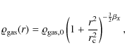
calculate the total gravitating mass using
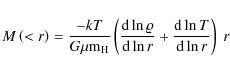
(Fabricant et al. 1980). Here,
![]() is
the mass of the hydrogen atom, and
is
the mass of the hydrogen atom, and ![]() the mean
molecular weight (assuming a fully ionised plasma with primordial
element abundances). The total density is the sum of two components
with the parameters given in Table 1 of Ikebe et al.:
the mean
molecular weight (assuming a fully ionised plasma with primordial
element abundances). The total density is the sum of two components
with the parameters given in Table 1 of Ikebe et al.:
![]() ,
,
![]() ,
,
![]()
![]() ,
,
![]() ,
and
,
and ![]() .
Since we assume that the gas is isothermal
(
.
Since we assume that the gas is isothermal
(
![]() ),
the second term in Eq. (24)
vanishes. Figure 21
shows the velocity dispersion
profiles expected for the blue and red GC subpopulations (assuming
constant anisotropy parameters of
-0.5,0,+0.5) for the mass profile
given in Eq. (24)
and plotted in Fig. 22.
Indeed,
the modelled velocity dispersion profiles show a dip near
),
the second term in Eq. (24)
vanishes. Figure 21
shows the velocity dispersion
profiles expected for the blue and red GC subpopulations (assuming
constant anisotropy parameters of
-0.5,0,+0.5) for the mass profile
given in Eq. (24)
and plotted in Fig. 22.
Indeed,
the modelled velocity dispersion profiles show a dip near
![]()
![]() ,
but the feature is quite shallow and appears to be
at variance with the findings for the red GCs.
,
but the feature is quite shallow and appears to be
at variance with the findings for the red GCs.
The mass profiles derived by Paolillo et al. (2002) would lead to more pronounced features in the predicted velocity dispersion profiles. Note however that a simple isothermal profile based on the gas density distribution ignoring the offsets of the different components (shown as thick line in their Fig. 15) leads to a non-monotonic (i.e. unphysical) density-profile at the transition from the galaxy to the cluster component.
![\begin{figure}
\par {\includegraphics[width=7.6cm,clip]{12482f41.eps} }\end{figure}](/articles/aa/full_html/2010/05/aa12482-09/img381.png)
|
Figure 21:
Comparison to the ``nested halo'' mass profile by
Ikebe et al. (1996).
Here, we plot the dispersion profiles expected for
their Model 1, see text for details. The thick curves are the
dispersion profiles for the blue GCs, where the solid and dashed lines
correspond to |
| Open with DEXTER | |
Figure 22 compares the mass profiles derived in this study (shown as solid and dot-dashed lines) with the X-ray mass profiles presented by Paolillo et al. (2002) and Ikebe et al. (1996). Within the central 100 Mpc, where the vast majority of our dynamical probes is found, the preferred mass profiles derived in this study agree well with the Ikebe et al. (1996) mass model, although we do not find any signs for the transition from galaxy to cluster halo in our kinematic data.
![\begin{figure}
\par {\includegraphics[width=7.6cm,clip]{12482f42.eps} }\end{figure}](/articles/aa/full_html/2010/05/aa12482-09/img385.png)
|
Figure 22:
Comparison to X-ray measurements. The grey area shows the
range of the mass models presented by Paolillo
et al. (2002). The thick
solid line shows the mass derived by Ikebe
et al. (1996) (their Model 1).
The thin solid line indicates the mass profile derived in
Paper I.
The dash-dotted curves are the two halos presented in
Richtler et al. (2008):
the more massive one (labelled R1) has the
parameters |
| Open with DEXTER | |
12 Conclusions
Using the largest data set of globular cluster (GC) radial velocities
available to date, we revisit and extend the investigation of the
kinematical and dynamical properties of the NGC 1399 GC system
with
respect to Richtler et al. (2004,
Paper I). We
measure about 700 GC radial velocities out to approximately
![]() (in
Paper I we reached 40 kpc). To
this sample we add 56 GC velocities from Bergond et al.
(2007, B+07) which go as
far out as 200 kpc.
(in
Paper I we reached 40 kpc). To
this sample we add 56 GC velocities from Bergond et al.
(2007, B+07) which go as
far out as 200 kpc.
Our main
findings are the following: there is no significant rotation signal
among the red (metal-rich) subpopulation. We find rotation around
the minor axis for the blue (metal-poor) clusters in a radial
interval of
![]() (i.e.
(i.e.
![]() ),
however weak. The blue and red clusters form
two kinematically distinct subpopulations rather
than showing a continuum of
kinematical properties.
),
however weak. The blue and red clusters form
two kinematically distinct subpopulations rather
than showing a continuum of
kinematical properties.
The red clusters correspond under various kinematical aspects to the stellar field populations.
Their velocity dispersion declines outwards and their velocity distribution suggests orbital isotropy.
The jump to the higher dispersion of the blue clusters occurs
at a
colour (
![]() ), which is also suggested by
the morphology
of the colour distribution. The blue GCs, however, show a more
complex behaviour. Their velocity dispersion profile is not as smooth
as that of the red GCs. There exist very high/low individual
velocities, which suggest very large apogalactic distances, as already
found in Paper I. These objects seem to belong to an
intergalactic
cluster population, which may be made up of GCs stemming from
disrupted dwarfs and GCs stripped off neighbouring galaxies during
close encounters.
), which is also suggested by
the morphology
of the colour distribution. The blue GCs, however, show a more
complex behaviour. Their velocity dispersion profile is not as smooth
as that of the red GCs. There exist very high/low individual
velocities, which suggest very large apogalactic distances, as already
found in Paper I. These objects seem to belong to an
intergalactic
cluster population, which may be made up of GCs stemming from
disrupted dwarfs and GCs stripped off neighbouring galaxies during
close encounters.
We performed a Jeans analysis in order to constrain the mass profile (stellar plus dark). We found it difficult to find a dark halo which simultaneously accounts for the red and the blue clusters, which again argues for a different dynamical history.
The dark NFW-halo which was found to represent the kinematics
of the
red GCs (
![]() )
and the stellar velocity dispersion
profile presented by Saglia
et al. (2000) (
)
and the stellar velocity dispersion
profile presented by Saglia
et al. (2000) (
![]() ),
our Model a10, has the parameters
),
our Model a10, has the parameters
![]() and
and
![]() .
The virial mass is
.
The virial mass is
![]() .
.
Including the velocities from B+07, (Model b10)
yields a
slightly more massive halo
(
![]() and
and
![]() ,
and a virial mass
,
and a virial mass
![]() ).
).
These NFW halos, which were found to represent the observations, are marginally less massive than the one from Paper I. The total mass profile fits agree reasonably well with the X-ray based mass profiles out to 80 kpc. However, our model halos when extrapolated stay significantly below the X-ray masses. Moreover, we do not see the transition from the galaxy halo to the cluster halo claimed to be present in the X-ray data.
We argue that these findings are consistent with a scenario
where the
red GCs are formed together with the bulk of the field population, most
probably in early multiple mergers with many progenitors
involved. This is consistent with the NGC 1399 GCs being
predominantly old (Hempel
et al. 2007; Forbes et al. 2001a; Kissler-Patig
et al. 1998; Kundu et al. 2005), with
ages very
similar to the stellar age of NGC 1399 (
![]() Gyr,
Trager et al. 2000)
Gyr,
Trager et al. 2000)
A large part of the blue GC population has been acquired by accretion processes, most plausibly through dwarf galaxies during the assembly of the Fornax cluster. Moreover, there should be a significant population of intra-cluster GCs.
AcknowledgementsWe thank the anonymous referee for helpful comments. We also thank Mike Fellhauer for fruitful discussions. Y.S. acknowledges support from a German Science Foundation Grant (DFG-Projekt HI-855/2). T.R. and A.J.R. acknowledge support from the Chilean Center for Astrophysics, FONDAP No. 15010003. A.J.R. was further supported by the National Science Foundation grants AST-0507729 and AST-0808099. This research has made use of the NASA/IPAC Extragalactic Database (NED) which is operated by the Jet Propulsion Laboratory, California Institute of Technology, under contract with the National Aeronautics and Space Administration.
Appendix A: Radial velocity dispersion profiles
Table A.1: Velocity dispersion profiles for fixed annular bins (cf. Fig. 13, middle panels).
Table A.2: Velocity dispersion profiles for the subsets of our data used for the Jeans modelling.
References
- Abramowitz, M., & Stegun, I. A. 1964, Handbook of Mathematical Functions with Formulas, Graphs, and Mathematical Tables, ninth dover printing, tenth gpo printing edn. (New York: Dover) [Google Scholar]
- Ashman, K. M., & Zepf, S. E. 1992, ApJ, 384, 50 [NASA ADS] [CrossRef] [Google Scholar]
- Avni, Y. 1976, ApJ, 210, 642 [NASA ADS] [CrossRef] [Google Scholar]
- Bassino, L. P., Faifer, F. R., Forte, J. C., et al. 2006, A&A, 451, 789 (B+06) [NASA ADS] [CrossRef] [EDP Sciences] [Google Scholar]
- Baum, W. A. 1955, PASP, 67, 328 [NASA ADS] [CrossRef] [Google Scholar]
- Beasley, M. A., Baugh, C. M., Forbes, D. A., Sharples, R. M., & Frenk, C. S. 2002, MNRAS, 333, 383 [NASA ADS] [CrossRef] [MathSciNet] [Google Scholar]
- Bedin, L. R., Piotto, G., Anderson, J., et al. 2004, ApJ, 605, L125 [NASA ADS] [CrossRef] [Google Scholar]
- Bekki, K., Beasley, M. A., Brodie, J. P., & Forbes, D. A. 2005, MNRAS, 363, 1211 [NASA ADS] [CrossRef] [Google Scholar]
- Bekki, K., Forbes, D. A., Beasley, M. A., & Couch, W. J. 2003, MNRAS, 344, 1334 [Google Scholar]
- Bellazzini, M., Ferraro, F. R., & Ibata, R. 2003, AJ, 125, 188 [NASA ADS] [CrossRef] [Google Scholar]
- Bergond, G., Athanassoula, E., Leon, S., et al. 2007, A&A, 464, L21 (B+07) [NASA ADS] [CrossRef] [EDP Sciences] [Google Scholar]
- Blakeslee, J. P., Tonry, J. L., & Metzger, M. R. 1997, AJ, 114, 482 [NASA ADS] [CrossRef] [Google Scholar]
- Brodie, J. P., & Strader, J. 2006, ARA&A, 44, 193 [NASA ADS] [CrossRef] [Google Scholar]
- Bullock, J. S., Kolatt, T. S., Sigad, Y., et al. 2001, MNRAS, 321, 559 [Google Scholar]
- Burkert, A. 1995, ApJ, 447, L25 [NASA ADS] [CrossRef] [Google Scholar]
- Côté, P., McLaughlin, D. E., Hanes, D. A., et al. 2001, ApJ, 559, 828 [NASA ADS] [CrossRef] [Google Scholar]
- Côté, P., McLaughlin, D. E., Cohen, J. G., & Blakeslee, J. P. 2003, ApJ, 591, 850 [NASA ADS] [CrossRef] [Google Scholar]
- Catelan, M. 2009, Ap&SS, 18 [Google Scholar]
- Churazov, E., Forman, W., Vikhlinin, A., et al. 2008, MNRAS, 388, 1062 [NASA ADS] [CrossRef] [Google Scholar]
- Cohen, J. G., Blakeslee, J. P., & Ryzhov, A. 1998, ApJ, 496, 808 [NASA ADS] [CrossRef] [Google Scholar]
- Cohen, J. G., Blakeslee, J. P., & Côté, P. 2003, ApJ, 592, 866 [NASA ADS] [CrossRef] [Google Scholar]
- Cohen, J. G., & Ryzhov, A. 1997, ApJ, 486, 230 [NASA ADS] [CrossRef] [Google Scholar]
- Colavitti, E., Pipino, A., & Matteucci, F. 2009, A&A, 499, 409 [NASA ADS] [CrossRef] [EDP Sciences] [Google Scholar]
- Collins, C. A., Stott, J. P., Hilton, M., et al. 2009, Nature, 458, 603 [NASA ADS] [CrossRef] [PubMed] [Google Scholar]
- Côté, P. 1999, AJ, 118, 406 [NASA ADS] [CrossRef] [Google Scholar]
- Côté, P., Marzke, R. O., & West, M. J. 1998, ApJ, 501, 554 [NASA ADS] [CrossRef] [Google Scholar]
- Côté, P., West, M. J., & Marzke, R. O. 2002, ApJ, 567, 853 [NASA ADS] [CrossRef] [Google Scholar]
- D'Agostino, R. B., & Stephens, M. A. 1986, Goodness-of-fit techniques (New York, NY, USA: Marcel Dekker, Inc.) [Google Scholar]
- di Matteo, P., Bournaud, F., Martig, M., et al. 2008, A&A, 492, 31 [NASA ADS] [CrossRef] [EDP Sciences] [Google Scholar]
- Diemand, J., Zemp, M., Moore, B., Stadel, J., & Carollo, C. M. 2005, MNRAS, 364, 665 [NASA ADS] [CrossRef] [Google Scholar]
- Dirsch, B., Richtler, T., Geisler, D., et al. 2003, AJ, 125, 1908 (D+03) [NASA ADS] [CrossRef] [Google Scholar]
- Dirsch, B., Richtler, T., Geisler, D., et al. 2004, AJ, 127, 2114 (D+04) [NASA ADS] [CrossRef] [Google Scholar]
- Drinkwater, M. J., Gregg, M. D., Holman, B. A., & Brown, M. J. I. 2001, MNRAS, 326, 1076 [Google Scholar]
- Evans, N. W., Wilkinson, M. I., Perrett, K. M., & Bridges, T. J. 2003, ApJ, 583, 752 [NASA ADS] [CrossRef] [Google Scholar]
- Fabricant, D., Lecar, M., & Gorenstein, P. 1980, ApJ, 241, 552 [NASA ADS] [CrossRef] [Google Scholar]
- Ferguson, H. C. 1989, AJ, 98, 367 [Google Scholar]
- Ferguson, H. C., & Sandage, A. 1989, ApJ, 346, L53 [NASA ADS] [CrossRef] [Google Scholar]
- Forbes, D. A., Brodie, J. P., & Grillmair, C. J. 1997, AJ, 113, 1652 [NASA ADS] [CrossRef] [Google Scholar]
- Forbes, D. A., Grillmair, C. J., Williger, G. M., Elson, R. A. W., & Brodie, J. P. 1998, MNRAS, 293, 325 [NASA ADS] [CrossRef] [Google Scholar]
- Forbes, D. A., Beasley, M. A., Brodie, J. P., & Kissler-Patig, M. 2001a, ApJ, 563, L143 [NASA ADS] [CrossRef] [Google Scholar]
- Forbes, D. A., Georgakakis, A. E., & Brodie, J. P. 2001b, MNRAS, 325, 1431 [NASA ADS] [CrossRef] [Google Scholar]
- Gebhardt, K., Lauer, T. R., Pinkney, J., et al. 2007, ApJ, 671, 1321 [NASA ADS] [CrossRef] [Google Scholar]
- Gentile, G., Salucci, P., Klein, U., & Granato, G. L. 2007, MNRAS, 375, 199 [NASA ADS] [CrossRef] [Google Scholar]
- Grillmair, C. J., Freeman, K. C., Bicknell, G. V., et al. 1994, ApJ, 422, L9 [NASA ADS] [CrossRef] [Google Scholar]
- Harris, W. E., & Racine, R. 1979, ARA&A, 17, 241 [NASA ADS] [CrossRef] [Google Scholar]
- Heisler, J., Tremaine, S., & Bahcall, J. N. 1985, ApJ, 298, 8 [NASA ADS] [CrossRef] [Google Scholar]
- Helmi, A. 2008, A&ARv, 15, 145 [NASA ADS] [Google Scholar]
- Hempel, M., Kissler-Patig, M., Puzia, T. H., & Hilker, M. 2007, A&A, 463, 493 [NASA ADS] [CrossRef] [EDP Sciences] [Google Scholar]
- Hilker, M., & Richtler, T. 2000, A&A, 362, 895 [NASA ADS] [Google Scholar]
- Hilker, M., Infante, L., & Richtler, T. 1999, A&AS, 138, 55 [NASA ADS] [CrossRef] [EDP Sciences] [Google Scholar]
- Hilker, M., Kayser, A., Richtler, T., & Willemsen, P. 2004, A&A, 422, L9 [NASA ADS] [CrossRef] [EDP Sciences] [Google Scholar]
- Hou, A., Parker, L. C., Harris, W. E., & Wilman, D. J. 2009, ApJ, 702, 1199 [NASA ADS] [CrossRef] [Google Scholar]
- Huchra, J., & Brodie, J. 1987, AJ, 93, 779 [NASA ADS] [CrossRef] [Google Scholar]
- Ihaka, R., & Gentleman, R. 1996, J. Comput. Graph. Stat., 5, 299 [Google Scholar]
- Ibata, R., Irwin, M., Lewis, G. F., & Stolte, A. 2001, ApJ, 547, L133 [NASA ADS] [CrossRef] [Google Scholar]
- Ikebe, Y., Ezawa, H., Fukazawa, Y., et al. 1996, Nature, 379, 427 [NASA ADS] [CrossRef] [Google Scholar]
- Jones, C., Stern, C., Forman, W., et al. 1997, ApJ, 482, 143 [Google Scholar]
- Kelson, D. D., Zabludoff, A. I., Williams, K. A., et al. 2002, ApJ, 576, 720 [NASA ADS] [CrossRef] [Google Scholar]
- Kissler-Patig, M., Richtler, T., Storm, J., & della Valle, M. 1997, A&A, 327, 503 [NASA ADS] [Google Scholar]
- Kissler-Patig, M., Brodie, J. P., Schroder, L. L., et al. 1998, AJ, 115, 105 [NASA ADS] [CrossRef] [Google Scholar]
- Kundu, A., & Whitmore, B. C. 2001a, AJ, 121, 2950 [NASA ADS] [CrossRef] [Google Scholar]
- Kundu, A., & Whitmore, B. C. 2001b, AJ, 122, 1251 [NASA ADS] [CrossRef] [Google Scholar]
- Kundu, A., Zepf, S. E., Hempel, M., et al. 2005, ApJ, 634, L41 [NASA ADS] [CrossRef] [Google Scholar]
- Larsen, S. S., & Richtler, T. 2000, A&A, 354, 836 [NASA ADS] [Google Scholar]
- Larsen, S. S., Brodie, J. P., Huchra, J. P., Forbes, D. A., & Grillmair, C. J. 2001, AJ, 121, 2974 [NASA ADS] [CrossRef] [Google Scholar]
- Lee, Y.-W., Gim, H. B., & Casetti-Dinescu, D. I. 2007, ApJ, 661, L49 [NASA ADS] [CrossRef] [Google Scholar]
- Machacek, M., Dosaj, A., Forman, W., et al. 2005, ApJ, 621, 663 [NASA ADS] [CrossRef] [Google Scholar]
- Makishima, K., Ezawa, H., Fukuzawa, Y., et al. 2001, PASJ, 53, 401 [NASA ADS] [CrossRef] [EDP Sciences] [Google Scholar]
- Mamon, G. A., & okas, E. L. 2005, MNRAS, 363, 705 [NASA ADS] [CrossRef] [Google Scholar]
- Mihos, J. C., & Hernquist, L. 1996, ApJ, 464, 641 [NASA ADS] [CrossRef] [Google Scholar]
- Minniti, D., Kissler-Patig, M., Goudfrooij, P., & Meylan, G. 1998, AJ, 115, 121 [NASA ADS] [CrossRef] [Google Scholar]
- Navarro, J. F., Frenk, C. S., & White, S. D. M. 1997, ApJ, 490, 493 [NASA ADS] [CrossRef] [Google Scholar]
- Paolillo, M., Fabbiano, G., Peres, G., & Kim, D.-W. 2002, ApJ, 565, 883 [NASA ADS] [CrossRef] [Google Scholar]
- Peng, E. W., Ford, H. C., & Freeman, K. C. 2004, ApJS, 150, 367 [NASA ADS] [CrossRef] [Google Scholar]
- Peng, E. W., Jordán, A., Côté, P., et al. 2006, ApJ, 639, 95 [NASA ADS] [CrossRef] [Google Scholar]
- Perea, J., del Olmo, A., & Moles, M. 1990, A&A, 237, 319 [NASA ADS] [Google Scholar]
- Pipino, A., D'Ercole, A., & Matteucci, F. 2008, A&A, 484, 679 [NASA ADS] [CrossRef] [EDP Sciences] [Google Scholar]
- Press, W. H., Flannery, B. P., Teukolsky, S. A., & Vetterling, W. T. 1992, Numerical Recipes in C: The Art of Scientific Computing (Cambridge University Press) [Google Scholar]
- Pryor, C., & Meylan, G. 1993, in Structure and Dynamics of Globular Clusters, ASP Conf. Ser., 50, 357 [Google Scholar]
- Racine, R. 1968, JRASC, 62, 367 [NASA ADS] [Google Scholar]
- Renzini, A. 2006, ARA&A, 44, 141 [NASA ADS] [CrossRef] [Google Scholar]
- Richtler, T. 2006, Bull. Astr. Soc. India, 34, 83 [Google Scholar]
- Richtler, T., Dirsch, B., Gebhardt, K., et al. 2004, AJ, 127, 2094 (Paper I) [NASA ADS] [CrossRef] [Google Scholar]
- Richtler, T., Grebel, E. K., Domgoergen, H., Hilker, M., & Kissler, M. 1992, A&A, 264, 25 [NASA ADS] [Google Scholar]
- Richtler, T., Schuberth, Y., Hilker, M., et al. 2008, A&A, 478, L23 [NASA ADS] [CrossRef] [EDP Sciences] [Google Scholar]
- Romanowsky, A. J., Strader, J., Spitler, L. R., et al. 2009, AJ, 137, 4956 [NASA ADS] [CrossRef] [Google Scholar]
- Royston, P. 1982, Applied Statistics, 115 [Google Scholar]
- Saglia, R. P., Kronawitter, A., Gerhard, O., & Bender, R. 2000, AJ, 119, 153 [NASA ADS] [CrossRef] [Google Scholar]
- Saha, P., Bicknell, G. V., & McGregor, P. J. 1996, ApJ, 467, 636 [NASA ADS] [CrossRef] [Google Scholar]
- Schuberth, Y., Richtler, T., Dirsch, B., et al. 2006, A&A, 459, 391 [NASA ADS] [CrossRef] [EDP Sciences] [Google Scholar]
- Schuberth, Y., Richtler, T., Bassino, L., & Hilker, M. 2008, A&A, 477, L9 [NASA ADS] [CrossRef] [EDP Sciences] [Google Scholar]
- Schweizer, F. 2006, in Globular clusters-Guide to Galaxies, ed. T. Richtler, & S. Larsen (Berlin, Heidelberg: Springer), 2009 [arXiv:astro-ph/0606036] [Google Scholar]
- Schweizer, F., & Seitzer, P. 1993, ApJ, 417, L29 [NASA ADS] [CrossRef] [Google Scholar]
- Shapiro, S. S., & Wilk, M. B. 1965, Biometrika, 3 [PubMed] [Google Scholar]
- Spitler, L. R., Forbes, D. A., Strader, J., Brodie, J. P., & Gallagher, J. S. 2008, MNRAS, 385, 361 [NASA ADS] [CrossRef] [Google Scholar]
- Stephens, M. A. 1974, J. American Statistical Association, 69, 730 [Google Scholar]
- Tal, T., van Dokkum, P. G., Nelan, J., & Bezanson, R. 2009, AJ, 138, 1417 [NASA ADS] [CrossRef] [Google Scholar]
- Tonry, J., & Davis, M. 1979, AJ, 84, 1511 [NASA ADS] [CrossRef] [Google Scholar]
- Toomre, A. 1977, in Evolution of Galaxies and Stellar Populations, ed. B. M. Tinsley, & R. B. Larson, 401 [Google Scholar]
- Trager, S. C., Faber, S. M., Worthey, G., & González, J. J. 2000, AJ, 120, 165 [NASA ADS] [CrossRef] [Google Scholar]
- van der Marel, R. P., & Franx, M. 1993, ApJ, 407, 525 [NASA ADS] [CrossRef] [Google Scholar]
- Venables, W. N., & Ripley, B. D. 2002, Modern Applied Statistics with S, 4th edn. (New York: Springer) [Google Scholar]
- Villanova, S., Piotto, G., King, I. R., et al. 2007, ApJ, 663, 296 [NASA ADS] [CrossRef] [Google Scholar]
- Wang, Z., Fazio, G. G., Ashby, M. L. N., et al. 2004, ApJS, 154, 193 [NASA ADS] [CrossRef] [Google Scholar]
- Weidner, C., Kroupa, P., & Larsen, S. S. 2004, MNRAS, 350, 1503 [NASA ADS] [CrossRef] [Google Scholar]
- Weijmans, A.-M., Krajnovic, D., van de Ven, G., et al. 2008, MNRAS, 383, 1343 [NASA ADS] [CrossRef] [Google Scholar]
- Whitmore, B. C., & Schweizer, F. 1995, AJ, 109, 960 [NASA ADS] [CrossRef] [EDP Sciences] [Google Scholar]
- Woodley, K. A., Harris, W. E., Beasley, M. A., et al. 2007, AJ, 134, 494 [NASA ADS] [CrossRef] [Google Scholar]
- Yoon, S.-J., Yi, S. K., & Lee, Y.-W. 2006, Science, 311, 1129 [NASA ADS] [CrossRef] [PubMed] [Google Scholar]
- Zinn, R. 1985, ApJ, 293, 424 [Google Scholar]
Footnotes
- ... NGC 1399
- Based on observations made with ESO Telescopes at the Paranal Observatories under programme ID 70.B-0174.
- ...
- Based on observations obtained at the Gemini Observatory, which is operated by the Association of Universities for Research in Astronomy, Inc., under a cooperative agreement with the NSF on behalf of the Gemini partnership: the National Science Foundation (United States), the Particle Physics and Astronomy Research Council (United Kingdom), the National Research Council (Canada), CONICYT (Chile), the Australian Research Council (Australia), CNPq (Brazil) and CONICET (Argentina).
- ...
- Tables B.1 and B.2 are only available in electronic form at the CDS via anonymous ftp to cdsarc.u-strasbg.fr (130.79.128.5) or via http://cdsweb.u-strasbg.fr/cgi-bin/qcat?J/A+A/513/A52
- ... camera
- The camera is mounted in the prime focus of the
4-m Blanco telescope and the field-of-view is
 .
.
- ... GCS
- This spectrum is part of the dataset analysed in Schuberth et al. (2009, in prep.).
- ...
velocities
- These authors give two velocities per spectrum,
 is the value derived with fxcor, and
  refers to
the direct line measurement (rvidlines).
refers to
the direct line measurement (rvidlines).
- ...
spectra
- The entry for 80:99 is a duplicate of 80:100. The object in slit 80:99 is a GC listed in Table 3 of D+04.
- ... range
- The data set includes foreground stars which do not fulfil the colour criteria for GC candidates because we extracted all spectra of a given mask, including those from the ``positioning slits'' used for the MXU mask alignment.
- ... (NED
- NASA/IPAC Extragalactic Database http://nedwww.ipac.caltech.edu
- ...
software
- R Development Core Team (Ihaka & Gentleman 1996) http://www.r-project.org.
All Tables
Table 1: Summary of VLT FORS 2/MXU observations (programme ID 70.B-0174).
Table 2: Summary of Gemini South GMOS observations (program IDs GS 2003B Q031 and GS 2004B Q029).
Table 3: Descriptive statistics of the line-of-sight velocity distribution.
Table 4: Rotation amplitudes and angles for the different subsamples.
Table 5: Globular cluster number density profiles.
Table 6: Jeans modelling best fit parameters.
Table A.1: Velocity dispersion profiles for fixed annular bins (cf. Fig. 13, middle panels).
Table A.2: Velocity dispersion profiles for the subsets of our data used for the Jeans modelling.
All Figures
|
|
Figure 1: Spatial distribution of spectroscopically confirmed GCs with respect to NGC 1399 (0,0). Dots represent GCs from Paper I. Circles and squares are the new GCs, measured using VLT/FORS 2 and Gemini/GMOS, respectively. North is to the top and East is to the left. The positions of NGC 1399 and NGC 1404 are marked by crosses. |
| Open with DEXTER | |
| In the text | |
|
|
Figure 2: Velocity uncertainties of the GC spectra as computed by fxcor. In both panels, crosses and dots represent blue and red GCs, respectively. Left panel: fxcor-uncertainties versus R-magnitude. Narrow and wide box-plots show the data for red and blue GCs, respectively. Right panel: fxcor-uncertainties vs. C-R colour overlaid with box-plots. The long-dashed line at C-R=1.55shows the division between blue and red GCs. In both panels, the short-dashed lines show the cuts used for assigning the quality flags (cf. Sect. 3.3). The boxes show the interquartile range (IQR), with the band marking the median. The whiskersextend to 1.5 times the IQR or the outermost data point, if closer. |
| Open with DEXTER | |
| In the text | |
|
|
Figure 3:
fxcor parameters and data classification.
The panels
show the histograms for all (unfilled histograms) and the
``Class A''
(grey histogram bars) GC spectra. Top left:
velocity
uncertainty, cut at |
| Open with DEXTER | |
| In the text | |
|
|
Figure 4:
Comparison to the velocity measurements by Dirsch
et al. (2004).
Velocity difference vs. R-magnitude. Dots
and crosses represent red
and blue GCs, respectively. The dashed (dotted) lines are drawn at
|
| Open with DEXTER | |
| In the text | |
|
|
Figure 5:
Duplicate measurements: velocity differences vs. apparent
magnitude. Crosses and dots are blue and red GCs,
respectively. Foreground stars are shown as diamonds. The error-bars
are the uncertainties of the two velocity measurements added in
quadrature. Small symbols indicate objects where at least one of the
spectra is classified as ``Class B''. In all panels, the
dashed lines
are drawn at |
| Open with DEXTER | |
| In the text | |
|
|
Figure 6:
Separating GCs from foreground stars: Upper panel:
C - R colour
vs. heliocentric velocity for objects with velocities
in the range
|
| Open with DEXTER | |
| In the text | |
|
|
Figure 7:
NGC 1399 spectroscopic GC sample: photometric properties and
spatial distribution. Upper left: GC luminosity
distribution
(bin width =0.2 mag). The dotted line at mR=23.3
indicates the
turn-over magnitude of the GCS. The thin solid, thick solid and
dashed lines show the kernel density estimates for all, the blue, and
the red GCs, respectively. Upper right panel:
colour
distribution. The dashed histogram shows the distribution of all
656 velocity-confirmed GCs for which MOSAIC photometry is
available, and the solid (unfilled) histogram are the GCs fainter than
mR=21.1,
and the grey histogram shows the distribution of the 144
brightest (
mR
< 21.1) GCs.
The dashed, solid and dot-dashed curves shows the respective kernel
density estimate for the same data; a bandwidth of 0.075 mag
was used
(same as histogram bins). The dotted line at
C
- R=1.55 indicates the limit
dividing blue from red GCs. Lower left: radial
distribution. The histogram (upper
sub-panel) shows all 693 GCs with velocity measurements. The
thin solid, thick solid and dashed lines show the kernel density
estimates for all, the blue and the red GCs, respectively. The radial
completeness, i.e. the number of GCs with velocity
measurements with
respect to the number of GC candidates (
0.9<C
- R<2.2) from the
D+03 photometry is shown in the lower sub-panel.
The black
dots (grey squares) show the values for a faint-end magnitude limit
of 23.0 (22.75). Lower right: azimuthal
distribution of the
GCs. The position angle (PA) is measured North over East, and the
dashed vertical lines indicate the photometric major axis of
NGC 1399
( |
| Open with DEXTER | |
| In the text | |
|
|
Figure 8:
Velocity dispersion as function of R-magnitude. For
all
GCs with mR>
20, the dispersion is calculated using Gaussian kernels
with a width of
|
| Open with DEXTER | |
| In the text | |
|
|
Figure 9: NGC 1399 GC velocities. Left panel: velocities vs. galactocentric distance for the blue and red GC sample (shown in the upper and lower sub-panel, respectively). Large and small dots show GCs with ``Class A'' and ``B'' velocity measurements, respectively. Objects brighter than mR=21.1 are marked by circles. The dashed line at 54 kpc shows the projected distance of NGC 1404. The solid and dashed horizontal lines indicate the systemic velocities of NGC 1399 and NGC 1404, respectively. Right: densities for the data points for the blue and red samples (BIII and RIII cf. 5.4) shown as grey-scale and contour plot. The blue subsample appears to exhibit substructure which is not present in the red. |
| Open with DEXTER | |
| In the text | |
|
|
Figure 10:
Interloper removal. Left: velocities
vs. distance
from NGC 1404. Crosses and dots represent blue and red GCs,
respectively. Large and small symbols refer to Class A and B
velocity
measurements, respectively. Bright GCs (
mR
< 21.1 mag) are marked
by a circle. The systemic velocities of NGC 1399 and
NGC 1404 are
shown as solid and dashed lines, respectively. The dotted line at
3 |
| Open with DEXTER | |
| In the text | |
|
|
Figure 11:
Velocity histograms. a): the unfilled histogram
shows all 693 GCs (AI). The solid
histogram bars are the
faint (mR>21.1)
GCs outside the 3 |
| Open with DEXTER | |
| In the text | |
|
|
Figure 12:
Rotation of the NGC 1399 GCS. Velocities versus position
angle. The upper panel shows the data for the
blue sample
BIII (i.e. the data after the removal of the
GCs in the
vicinity of NGC 1404 and the outlier rejection) for the
azimuthally
complete radial interval
|
| Open with DEXTER | |
| In the text | |
|
|
Figure 13: Velocity diagrams and line-of-sight velocity dispersion profiles. Upper left: radial velocity vs. galactocentric distance for the red GCs. Dots and circles show faint and bright ( mR < 21.1 mag) GCs, respectively. Large and small triangles are the data points from Bergond et al. (2007) with Class A and B velocity measurements, respectively (see text for details). Squares mark GCs rejected on account of their proximity to NGC 1404; crosses are the GCs removed by the TME rejection algorithm. The solid and dashed horizontal lines are the systemic velocities of NGC 1399 and NGC 1404, respectively. The vertical dashed line shows the (projected) distance of NGC 1404. The dotted vertical lines show the radial bins for which the dispersion shown in the middle panels is calculated. Upper right: the same for the blue GCs. Middle panels: the dispersion profiles for fixed radial bins. Circles are the values obtained for the full samples (RI and BI) prior to any interloper removal. Filled squares show the values after removing GCs in the vicinity of NGC 1404 and the outliers identified by the TME algorithm (samples RIII and BIII). The dispersion profiles for the extended samples (RV and BV) including the velocities from Bergond et al. (2007) are shown as diamonds. The labels in parentheses give the number of GCs in a given bin. Bottom panels: filled squares are the profiles for RIII and BIII obtained for a moving bin comprising 35 GCs. Diamonds show the same for the samples RV and BV. These moving-bin profiles which are used for the modelling in Sect. 10 are listed in Table A.2. |
| Open with DEXTER | |
| In the text | |
|
|
Figure 14: Comparison to the stellar kinematics presented by Saglia et al. (2000). Upper panel: line-of-sight velocity dispersion profiles. Diamonds show the stellar kinematics, dots and crosses are our measurements of the red (R III) and blue (B III) GCs, respectively. Lower panel: Gauss-Hermite parameter h4 (Eq. (6)) vs. projected radius. The values for the blue and red GCs are shown as long-dashed and dashed rectangle, respectively. The solid grey rectangle shows the value for the combined red and blue sample. The values derived from absorption-line spectroscopy by Saglia et al. (2000) are shown as diamonds, and the dashed line represents their best fit model (cf. their Fig. 5). |
| Open with DEXTER | |
| In the text | |
|
|
Figure 15: GC number density profiles. The data from B+06 are shown together with the fits to Eq. (10). Circles and squares represent the red and blue GCs, respectively. The fits to the red and the blue number density distributions are shown as dashed and solid line, respectively. The coefficients are listed in Table 5. The dashed and solid arrows indicate the core radii R0 as returned from the fits for the red and blue GCs, respectively. Diamonds show the surface brightness profile of NGC 1399, as given in Table 4 of D+03 (the data points have been shifted for comparison with the red GC number density profile). |
| Open with DEXTER | |
| In the text | |
|
|
Figure 16: Comparison between different deprojections of the surface brightness profile of NGC 1399: the dashed curve is the re-projection of the luminosity density profile as given in D+03 (Eq. (15)). The solid curve shows the fit to the data (Eq. (12)), which corresponds to there-projection of Eq. (14). |
| Open with DEXTER | |
| In the text | |
|
|
Figure 17:
Mass models (NFW halo): confidence level contours (68%, 90%, and 99%).
The x-axis plots the virial mass (
|
| Open with DEXTER | |
| In the text | |
|
|
Figure 18:
Best fit Jeans models (NFW halo). Left panel:
NGC 1399 GC data and modelled velocity dispersion profiles.
Crosses
and dots show the red (RIII) and blue (BIII)
velocity dispersion profiles (for a moving bin of 35 GCs,
cf. Fig. 13,
lower panels), respectively. The
thin curves are the best fit models obtained
for the red
(models a1-a3) and the blue GCs (models a4-a6)
separately. The thick lines (with labels) show
the dispersions
for the combined model for red and blue GCs (models a7
and
a8). Middle panel: the
same for the ``extended'' samples
including the Bergond
et al. (2007) measurements (samples RV
and
BV). Right panel: red
GCs and stars. Diamonds show
the stellar velocity dispersion (Saglia
et al. 2000), the red GCs
(RIII) are shown as dots. The thin lines are
the models for
the individual tracer populations, i.e. models c1
and c2
for the stars and models a1-a3 for the red GCs.
The thick
curves are the joint solutions, i.e. models a9
and a10.
In all panels, solid lines are isotropic models, and the models with
|
| Open with DEXTER | |
| In the text | |
|
|
Figure 19: Left panel: mass profiles derived for the GC dispersion profiles RIII and BIII. The thick lines with labels referring to the identifiers in Table 6 show the mass assuming an NFW-type dark halo. The cored Burkert halos are shown as thin curves with the same line style. For a given tracer population, the Burkert halo is less massive than the best-fit NFW halo. Right panel: the same for the extended data sets RV and BV (i.e. including velocities from B+07). In both panels, the dotted and dashed vertical lines indicate the radial distance of the outermost velocity dispersion data point for the red and blue GCs, respectively (cf. Table A.2). |
| Open with DEXTER | |
| In the text | |
|
|
Figure 20:
Upper panel: velocity dispersion as a
function of
C-R-colour. The data points
show the velocity dispersion for
the Class A GCs which are fainter than mR=21.1
(i.e. the union of samples
BIV and RIV) for
bins of |
| Open with DEXTER | |
| In the text | |
|
|
Figure 21:
Comparison to the ``nested halo'' mass profile by
Ikebe et al. (1996).
Here, we plot the dispersion profiles expected for
their Model 1, see text for details. The thick curves are the
dispersion profiles for the blue GCs, where the solid and dashed lines
correspond to |
| Open with DEXTER | |
| In the text | |
|
|
Figure 22:
Comparison to X-ray measurements. The grey area shows the
range of the mass models presented by Paolillo
et al. (2002). The thick
solid line shows the mass derived by Ikebe
et al. (1996) (their Model 1).
The thin solid line indicates the mass profile derived in
Paper I.
The dash-dotted curves are the two halos presented in
Richtler et al. (2008):
the more massive one (labelled R1) has the
parameters |
| Open with DEXTER | |
| In the text | |
Copyright ESO 2010
Current usage metrics show cumulative count of Article Views (full-text article views including HTML views, PDF and ePub downloads, according to the available data) and Abstracts Views on Vision4Press platform.
Data correspond to usage on the plateform after 2015. The current usage metrics is available 48-96 hours after online publication and is updated daily on week days.
Initial download of the metrics may take a while.