| Issue |
A&A
Volume 512, March-April 2010
|
|
|---|---|---|
| Article Number | A84 | |
| Number of page(s) | 10 | |
| Section | The Sun | |
| DOI | https://doi.org/10.1051/0004-6361/200913002 | |
| Published online | 09 April 2010 | |
Magnetic reconnection at 3D null points: effect of magnetic field asymmetry
A. K. Al-Hachami - D. I. Pontin
Division of Mathematics, University of Dundee, UK
Received 28 July 2009 / Accepted 23 January 2010
Abstract
Context. The magnetic field in many astrophysical plasmas,
for example in the solar corona, is known to have a highly complex -
and clearly three-dimensional - structure. Turbulent plasma motions in
high-![]() regions where field lines are anchored, such as the solar interior, can
store large amounts of energy in the magnetic field. This energy can
only be released when magnetic reconnection occurs. Reconnection may
only occur in locations where huge gradients of the magnetic field
develop, and one candidate for such locations are magnetic null points,
known to be abundant for example in the solar atmosphere. Reconnection
leads to changes in the topology of the magnetic field, and energy
being released as heat, kinetic energy and acceleration of particles.
Thus reconnection is responsible for many dynamic processes, for
instance flares and jets.
regions where field lines are anchored, such as the solar interior, can
store large amounts of energy in the magnetic field. This energy can
only be released when magnetic reconnection occurs. Reconnection may
only occur in locations where huge gradients of the magnetic field
develop, and one candidate for such locations are magnetic null points,
known to be abundant for example in the solar atmosphere. Reconnection
leads to changes in the topology of the magnetic field, and energy
being released as heat, kinetic energy and acceleration of particles.
Thus reconnection is responsible for many dynamic processes, for
instance flares and jets.
Aims. The aim of this paper is to investigate the properties of
magnetic reconnection at a 3D null point, with respect to their
dependence on the symmetry of the magnetic field around the null. In
particular we examine the rate of reconnection of magnetic flux at the
null point, as well as how the current sheet forms and its properties.
Methods. We use mathematical modelling and finite difference resistive MHD simulations.
Results. It is found that the basic structure of the mode of
magnetic reconnection considered is unaffected by varying the magnetic
field symmetry, that is, the plasma flow is found to cross both the
spine and fan of the null. However, the peak intensity and dimensions
of the current sheet are dependent on the symmetry/asymmetry of the
field lines. As a result, the reconnection rate is also found to be
strongly dependent on the field asymmetry.
Conclusions. The symmetry/asymmetry of the magnetic field in the
vicinity of a magnetic null can have a profound effect on the geometry
of any associated reconnection region, and the rate at which the
reconnection process proceeds.
Key words: magnetohydrodynamics (MHD) - magnetic reconnection - Sun: corona - Sun: magnetic topology
1 Intoduction
Magnetic reconnection is the breaking and topological or geometrical rearrangement of the magnetic field lines in a plasma. The magnetic field plays a fundamental role in many of the phenomena that occur in the plasma. It is not surprising that three-dimensional (3D) magnetic fields are more complex than two-dimensional ones. It is known from observations that magnetic reconnection occurs in abundance in astrophysical plasmas. However, due to the very low plasma resistivity, reconnection may only occur where very intense currents (``current sheets'') develop. One of the most fundamental questions that must be answered to determine the locations and mechanisms of energy release in astrophysical plasmas is therefore: where may such currents develop?It is now becoming clear that the magnetic field in the solar atmosphere has a highly complex structure. Two major candidates that have been proposed as sites of current sheet formation in such a complex magnetic field are 3D nulls points, and associated separator field lines (Pontin & Craig 2005; Priest & Titov 1996; Longcope 1996; Longcope & Cowley 1996; Klapper et al. 1996; Lau & Finn 1990; Galsgaard & Nordlund 1997; Longcope 2001) - field lines that link two nulls. We focus here on reconnection at isolated 3D nulls. Indications are that an abundance of 3D nulls is present in the solar corona (Régnier et al. 2008; Longcope & Parnell 2009), which have been suggested as likely sites for coronal heating (e.g. Priest et al. 2005). Moreover, recent observations suggest that reconnection at such nulls may play an important role in jets (Török et al. 2009; Pariat et al. 2009) solar flares (e.g. Luoni et al. 2007; Masson et al. 2009) and coronal mass ejections (e.g. Ugarte-Urra et al. 2007; Barnes 2007). Furthermore, recently the first in-situ observations have been made by the Cluster spacecraft of single and multiple 3D magnetic nulls in the Earth's magnetotail (e.g. Xiao et al. 2006). The observations further suggest that these nulls may be playing an important role in the reconnection process occurring in the magnetotail. Though magnetic field measurements in other astrophysical objects further afield are difficult, it is almost certain that similar reconnection processes at 3D nulls also occur there.
To find the local magnetic structure about a null point, we
consider the magnetic field in the vicinity of null point where the
field vanishes (![]() ).
If the null point is taken to be situated at the origin and, in
addition, we assume we are sufficiently close to the null, then the
magnetic field may be expressed as
).
If the null point is taken to be situated at the origin and, in
addition, we assume we are sufficiently close to the null, then the
magnetic field may be expressed as
where
Unlike in two dimensions, reconnection can occur in 3D either at a null point or in the absence of nulls (Priest & Forbes 2000; Schindler et al. 1988; Démoulin 2006). What's more, the nature of reconnection in 3D has been shown to be fundamentally different from 2D reconnection (Priest et al. 2003). The nature of magnetic reconnection in the absence of a three-dimensional null point has been discussed by Hesse (1991) and Hornig & Priest (2003). The kinematics of steady reconnection at three dimensional null points have been studied by Priest & Titov (1996) when ![]() .
Later, Pontin et al. (2004,2005)
improved this model by adding a finite resistivity, localised around
the null point. Two distinct cases were considered, in which the
current (
.
Later, Pontin et al. (2004,2005)
improved this model by adding a finite resistivity, localised around
the null point. Two distinct cases were considered, in which the
current (![]() )
was directed parallel to first the spine and second the fan plane of
the null. The structures of the two solutions were found to differ
greatly, and as a result, the reconnection rate, calculated by
integrating the E|| along field lines, represents very different behaviors of the flux for the two cases. In the first case, in which
)
was directed parallel to first the spine and second the fan plane of
the null. The structures of the two solutions were found to differ
greatly, and as a result, the reconnection rate, calculated by
integrating the E|| along field lines, represents very different behaviors of the flux for the two cases. In the first case, in which ![]() was directed parallel to the spine, a type of rotational flux
mis-matching was found, with no flow being present across either the
spine or the fan of the null point. On the other hand, when
was directed parallel to the spine, a type of rotational flux
mis-matching was found, with no flow being present across either the
spine or the fan of the null point. On the other hand, when ![]() was directed parallel to the fan surface, it was found that magnetic
flux is transported through the spine line and the fan plane, in a
process much more conceptually similar to the 2D case. In this case it
can be shown that the reconnection rate gives a measure of the rate of
flux transport across the separatrix surface of the null (Pontin et al. 2005). The case in which
was directed parallel to the fan surface, it was found that magnetic
flux is transported through the spine line and the fan plane, in a
process much more conceptually similar to the 2D case. In this case it
can be shown that the reconnection rate gives a measure of the rate of
flux transport across the separatrix surface of the null (Pontin et al. 2005). The case in which ![]() is parallel to the spine corresponds to one pair of complex conjugate eignevalues, whereas when
is parallel to the spine corresponds to one pair of complex conjugate eignevalues, whereas when ![]() is parallel to the fan the eignevalues are all real. In each of these
investigations only the azimuthually symmetric case was considered,
that is the case in which the magnetic field in the fan plane is
isotropic. In this paper we focus on the case where
is parallel to the fan the eignevalues are all real. In each of these
investigations only the azimuthually symmetric case was considered,
that is the case in which the magnetic field in the fan plane is
isotropic. In this paper we focus on the case where ![]() is parallel to the fan surface (real eigenvalues), and for the first
time consider magnetic reconnection at a generic non-symmetric magnetic
null point, i.e. a null for which the fan eigenvalues are not
equal. The different modes of reconnection that occur in practice in a
plasma (when the full set of MHD equations are considered) have
recently been classified by Priest & Pontin (2009). In terms of the framework they have set up, the mode of reconnection considered here is termed spine-fan reconnection. In a future paper we will go on to generalise the complex conjugate eigenvalue case.
is parallel to the fan surface (real eigenvalues), and for the first
time consider magnetic reconnection at a generic non-symmetric magnetic
null point, i.e. a null for which the fan eigenvalues are not
equal. The different modes of reconnection that occur in practice in a
plasma (when the full set of MHD equations are considered) have
recently been classified by Priest & Pontin (2009). In terms of the framework they have set up, the mode of reconnection considered here is termed spine-fan reconnection. In a future paper we will go on to generalise the complex conjugate eigenvalue case.
In Sects. 2 and 3, we describe a kinematic model for reconnection at a non-symmetric null point, comparing our results with those of Pontin et al. (2005). In Sect. 4 we describe the results of a related resistive magnetohydrodynamic (MHD) numerical simulation, and in Sect. 5 we present our conclusions.
2 Kinematic solution - method
2.1 The model
The subject of magnetic reconnection is a complex one, and its study is still in the early stages. Therefore, one approach that is used to try to understand the properties of this process is to consider a reduced set of the MHD equations. There are a number of analytical 3D solutions, which are described by Hornig & Priest (2003) and Wilmot-Smith et al. (2009,2006), where there is no null point of the magnetic field, as well as the solutions in the presence of a null mentioned above (Pontin et al. 2004; Priest & Pontin 2009; Pontin et al. 2005). These solutions are kinematic reconnection, that is they satisfy Maxwell's equations, as well as the induction equation. This approach can give great insight into the topological structure of a magnetic reconnection process occurring at an isolated diffusion region (Schindler et al. 1988). After investigating the properties of the solutions of this subset of the MHD equations, we go on in Sect. 4 to examine which properties survive when the full set of resistive MHD equations is solved.
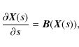
We seek a solution to the kinematic, steady, resistive MHD equations in
the locality of a magnetic null point. That is, we solve
As discussed above, here we consider a null point with current directed parallel to the fan plane. We choose the magnetic field to be

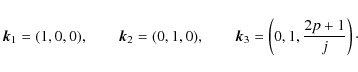
where p is a parameter (here we restrict ourselves to the case p>0). This generalises the previous work by Pontin et al. (2005), who considered only the case where the field in the fan plane (z=0) is azimuthally symmetric, corresponding to p=1. For convenience we will write
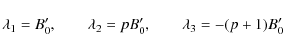
with corresponding eigenvectors
It is clear from the above that the fan plane is defined by
For the chosen magnetic field (6), closed-form expressions for the equations of
magnetic field lines can be found, by solving
where the parameter s runs along field lines, to give


The inverse of Eqs. (8-10) are


which describes the equations of the magnetic field lines in terms of some initial coordinates
![\begin{figure}
\par\subfigure[]{\includegraphics[width=7cm]{13002f1a.eps} }
\par...
...s} }
\par\subfigure[]{\includegraphics[width=7cm]{13002f1c.eps} }\end{figure}](/articles/aa/full_html/2010/04/aa13002-09/img36.png)
|
Figure 1: The structure of the magnetic null point with j=1 and different values of p: a) p=0.5, b) p=1 and c) p=2. |
| Open with DEXTER | |
We proceed to solve (2-5) as follows. From Eq. (3) we can write, in general,
![]() where
where ![]() is a scalar potential. Then the component of Eq. (2) parallel to B is
is a scalar potential. Then the component of Eq. (2) parallel to B is
![]() and we can calculate
and we can calculate ![]() by integrating along magnetic field lines:
by integrating along magnetic field lines:

where
and we then find the plasma velocity perpendicular to the magnetic field,

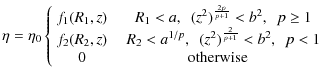
Now, in order to investigate the properties of magnetic reconnection in a fully 3D system, we impose a diffusion region that is spatially localised in 3D. This is the case relevant to astrophysical plasmas, which are known to be effectively ideal except in very small regions where energy release occurs. The diffusion region is chosen to be localised around the null point itself, in line with the results of past work which have shown that shearing motions tend to focus current in the vicinity of the null (Rickard & Titov 1996; Pontin et al. 2007; Pontin & Galsgaard 2007). We choose the resistivity to be localised, and take it to be of the form

|
||

|
(17) |
where
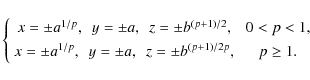
In order to integrate Eq. (14), we must choose a surface on which to start our integration (i.e. on which to set s=0) that intersects each field line once and only once, in order that ![]() is single-valued. We choose surfaces above and below the fan surface,
is single-valued. We choose surfaces above and below the fan surface, ![]() ,
constant. To simplify the mathematical expressions, and without loss of generality, we assume z0=b. Performing the calculation of
,
constant. To simplify the mathematical expressions, and without loss of generality, we assume z0=b. Performing the calculation of
![]() as described above yields two expressions for
as described above yields two expressions for ![]() ,
for z>0 and z<0. In order to match these two expressions at the fan plane, that is for
,
for z>0 and z<0. In order to match these two expressions at the fan plane, that is for ![]() to be smooth and continuous, and thus physically acceptable, we must set the value of
to be smooth and continuous, and thus physically acceptable, we must set the value of ![]() at
at
![]() (i.e.
(i.e. ![]() in Eq. (14)) to be
in Eq. (14)) to be

|
(18) |
where

3 Kinematic solution - analysis
3.1 Nature of reconnection
In order to determine the structure of the magnetic reconnection process, we will examine the plasma velocity perpendicular to the magnetic field (![\begin{figure}
\par\subfigure[]{\includegraphics[width=7.8cm]{13002f2a.eps} }
\p...
...} }
\par\subfigure[]{\includegraphics[width=7.8cm]{13002f2c.eps} }\end{figure}](/articles/aa/full_html/2010/04/aa13002-09/img69.png)
|
Figure 2:
Structure of the plasma flow across the spine and fan (black lines) in typical plane of constant x=0, where the grayed area is the diffusion region, for a) p=2, b) p=0.9, c) p=0.5, for parameters
|
| Open with DEXTER | |
3.2 Reconnection rate
It is generally accepted that magnetic reconnection plays a fundamental
role in many types of explosive astrophysical phenomena, for example
solar flares. Yet what determines the reconnection rate is still a
major problem and this is an important aspect of any reconnection
model. In general, the reconnection rate in 3D is defined by the
maximal value of

along any field line threading a spatially localised diffusion region D (e.g. Schindler et al. 1988). By symmetry, in this case

where the curve C2 lies along the x-axis, as shown in Fig. 3. Since the fan is a flux surface, the integral may equally well be performed along the curve C1, the curve C1 lying in the fan perpendicular to

from which it is clear that this reconnection rate measures the rate at which flux is transported across the fan surface by the flow in the ideal region (Pontin et al. 2005).
![\begin{figure}
\par\includegraphics[width=7cm,clip]{13002f3.eps}
\end{figure}](/articles/aa/full_html/2010/04/aa13002-09/img75.png)
|
Figure 3: The curves C1 and C2 joining two points on the x-axis, where the grayed area is the diffusion region, the arrows indicate the direction of field lines, for a=1. |
| Open with DEXTER | |


where
![\begin{figure}
\par\subfigure[]{\includegraphics[width=7.8 cm]{13002f4a.eps} }
\par\subfigure[]{\includegraphics[width=7.8 cm]{13002f4b.eps} }\end{figure}](/articles/aa/full_html/2010/04/aa13002-09/img80.png)
|
Figure 4:
Dependence of the reconnection rate on p, where the solid curve at a=1.5, dash-dotted curve at a=1, long dashed at a=0.5, for a) j=2j0, b)
j=j0 (p+1), and parameters
|
| Open with DEXTER | |
We will also consider the effect, in each of these cases, of taking different values for the parameter a, which controls the dimensions of the diffusion region. When a=1, the diffusion region is symmetric for all p, having circular cross-section in any plane of constant z. However, as stated above, the boundary of the diffusion region intersects each of the 3 coordinate axes at
Thus the diffusion region becomes asymmetric in the xy-plane when
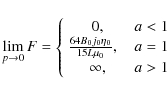
3.2.1 Reconnection rate as p


In the limit
![]() ,
we observe from (24) that the diffusion region becomes approximately symmetric (exactly symmetric if a=1). The following all holds for all values of a. For the two choices of dependence for our parameter j stated above, evaluating Eq. (23) we find
,
we observe from (24) that the diffusion region becomes approximately symmetric (exactly symmetric if a=1). The following all holds for all values of a. For the two choices of dependence for our parameter j stated above, evaluating Eq. (23) we find
![\begin{displaymath}\left. \lim_{p\to \infty} F ~ \right]_{{j=2j_0}} = 0
\end{displaymath}](/articles/aa/full_html/2010/04/aa13002-09/img84.png)
![\begin{displaymath}\left. \lim_{p\rightarrow \infty} F ~ \right]_{j=j_0 (p+1)} = \frac{4j_{0}B_{0}\eta_{0}}{L \mu_{0}}\cdot
\end{displaymath}](/articles/aa/full_html/2010/04/aa13002-09/img85.png)
Consider first the case where the parameter j is chosen to be a constant, j=2j0 (so that the current
By contrast, the reconnection rate approaches a constant finite value as
![]() when
j=j0 (p+1) (so that
when
j=j0 (p+1) (so that
![]() ). In this case the magnetic field is
). In this case the magnetic field is
![]() .
So the configuration is that of a 2D X-point with a uniform current (proportional to j0). As the diffusion region has only a finite extent along the direction of the current (
.
So the configuration is that of a 2D X-point with a uniform current (proportional to j0). As the diffusion region has only a finite extent along the direction of the current (
![]() ), the reconnection rate is finite. Note that as expected it is proportional to the parameters
), the reconnection rate is finite. Note that as expected it is proportional to the parameters
![]() and j0, where
and j0, where ![]() is the resistivity at the null, and
is the resistivity at the null, and
![]() is the current modulus.
is the current modulus.
3.2.2 Reconnection rate as p
0
We now turn to the opposite limit; ![]() .
Note that our two parameter choices j=2j0 and
j=j0(p+1) clearly reduce to the same situation (with j0 replaced by 2j0) as the limit is approached. Setting p=0 the magnetic field is
.
Note that our two parameter choices j=2j0 and
j=j0(p+1) clearly reduce to the same situation (with j0 replaced by 2j0) as the limit is approached. Setting p=0 the magnetic field is
![]() .
We note that this field contains a neutral line in 3D (along y=0)
which is anti-parallel to the direction of current flow - not a
configuration associated with 2D reconnection. In fact the limit of
Eq. (23) is not well defined for all choices of our parameters. Therefore we consider that p=0 is not a physically relevant parameter choice and consider only the limit
.
We note that this field contains a neutral line in 3D (along y=0)
which is anti-parallel to the direction of current flow - not a
configuration associated with 2D reconnection. In fact the limit of
Eq. (23) is not well defined for all choices of our parameters. Therefore we consider that p=0 is not a physically relevant parameter choice and consider only the limit ![]() .
.
As ![]() ,
the magnetic field in the fan plane parallel to the current vector becomes strong, while the
,
the magnetic field in the fan plane parallel to the current vector becomes strong, while the
![]() -component
becomes weak. Correspondingly, the flow across the fan surface becomes
isolated to a small region near the fan, and weakens, see Fig. 2. Furthermore, in this case the diffusion region D is highly anti-symmetric.
-component
becomes weak. Correspondingly, the flow across the fan surface becomes
isolated to a small region near the fan, and weakens, see Fig. 2. Furthermore, in this case the diffusion region D is highly anti-symmetric.
Evaluating Eq. (23) we find
(taking j=2j0). For a<1 the extent of D along the x-axis (direction of current flow) shrinks to zero. The result of the weak flow across the fan for small p is therefore that the reconnection rate also approaches zero when
The results discussed above show that depending on our choice of parameters there are various different ways in which the reconnection rate may depend on the asymmetry of the field (p). We now go on to perform simulations in the resistive MHD regime, in order to investigate which of these dependencies is relevant in a dynamically evolving plasma.
4 Resistive MHD simulations
4.1 Computational setup
We now proceed to test the results of the mathematical model
presented in the previous section by performing numerical simulations
which solve the full set of resistive MHD equations.
We solve the MHD equations in the following form
| |
= | (25) | |
| = | (26) | ||
| = | (27) | ||
| = | (28) | ||
| = | (29) | ||
| = | (30) |
where v, B, E,
We consider an isolated three dimensional null point within our
computational volume, which is driven from the boundary. We begin
initially with a potential magnetic field

taking B0=L=1 and

4.2 Current sheet
In order to simplify the discussion we will initially explain the behaviour of the current at one value of p (p=2). We first examine the temporal evolution of current in the volume. In the beginning the spine and fan are orthogonal, but then the angle between them begins to change, reaching a minimum value once the current sheet forms. In other words the null collapses from a perpendicular X-type null point, with the angle between the X becoming greatly reduced, see Fig. 5. After the boundary driving ceases the current begins to decrease again, and the spine and fan relax back towards their initial perpendicular state, see Fig. 7a.
![\begin{figure}
\par\mbox{\subfigure[]{\includegraphics[width=4.3cm]{13002f5a.eps...
...gure[]{\includegraphics[width=4cm]{13002f5c.eps} }\hspace*{2.3cm}}\end{figure}](/articles/aa/full_html/2010/04/aa13002-09/img123.png)
|
Figure 5:
Structure of the magnetic field for the run with p=2 a) at t=0, and b) at the time of maximum current (t=3.0),
once the magnetic field has locally collapsed to form a current sheet.
The black field lines are traced from around the spine for z>0, while the grey field lines are traced from z<0. c) Grayscale showing |
| Open with DEXTER | |
We now discuss how the current sheet formation, as described above, depends on the value of p. Figure 6 illustrates the dimensions of the current sheet for various values of p at the time when the current modulus is of maximum value. For the case investigated previously, p=1, the sheet was found to be approximately of equal dimensions along x and y, the two coordinate directions associated with the fan surface. Looking at Fig. 6 we see a large difference between the geometry of the current sheet at p=0.1 and at p=10 at the maximum current. We find the current sheet at p=0.1 is large, being very extended along the x-axis, that is, the direction along which ![]() and the parallel electric field lie. However, this length decreases when p is increased. The results suggest that when the value of p
approaches zero, the current sheet will grow indefinitely in the plane
perpendicular to the shear, i.e. the direction of current flow
through the null (x-direction). Note that with respect to the field strength in the fan plane, decreasing p corresponds to weaker magnetic field strength along the x-direction.
Thus the extension of the current sheet could be attributed to the fact
that the weak field region extends in that direction and the magnetic
field becomes less able to resist the collapse to form the current
layer. That is, when the magnetic field parallel to the current becomes
weaker there is less magnetic pressure associated with this ``guide
field'' component in the current sheet away from the null, and the
current sheet is able to extend further away from the null.
and the parallel electric field lie. However, this length decreases when p is increased. The results suggest that when the value of p
approaches zero, the current sheet will grow indefinitely in the plane
perpendicular to the shear, i.e. the direction of current flow
through the null (x-direction). Note that with respect to the field strength in the fan plane, decreasing p corresponds to weaker magnetic field strength along the x-direction.
Thus the extension of the current sheet could be attributed to the fact
that the weak field region extends in that direction and the magnetic
field becomes less able to resist the collapse to form the current
layer. That is, when the magnetic field parallel to the current becomes
weaker there is less magnetic pressure associated with this ``guide
field'' component in the current sheet away from the null, and the
current sheet is able to extend further away from the null.
![\begin{figure}
\par\mbox{\subfigure[]{\includegraphics[width=4cm]{13002f6a.eps} ...
...gure[]{\includegraphics[width=5cm]{13002f6e.eps} }\hspace*{1.5cm}}\end{figure}](/articles/aa/full_html/2010/04/aa13002-09/img124.png)
|
Figure 6:
Isosurfaces of |
| Open with DEXTER | |
4.3 Maximum current attained
| Figure 7:
a) Evolution of the maximum value of |
|
| Open with DEXTER | |
4.4 Reconnection rate
The nature of the plasma flow, and the resulting qualitative structure of the reconnection process, are found to be independent of the value of p. Specifically, we find plasma flow across both the spine line and fan plane of the null for all values of p. Figure 8 shows the plasma flow for two different values of p. Comparing with Fig. 2, we see that the trend for the geometry of the flow is the same as in the kinematic solution. Specifically, for large p, the flow exhibits a relatively symmetric stagnation structure (in the x=0 plane). For smaller p the flow across the fan becomes confined to a narrower region, and comparatively weaker with respect to the flow across the spine.![\begin{figure}
\par\subfigure[]{\includegraphics[width=5.5 cm]{13002f8a.eps} }
\par\subfigure[]{\includegraphics[width=5.5 cm]{13002f8b.eps} }\par\end{figure}](/articles/aa/full_html/2010/04/aa13002-09/img127.png)
|
Figure 8:
Plasma velocity in the x=0 plane for
|
| Open with DEXTER | |
In this section we calculate the reconnection rate, i.e. the amount of flux transported across the fan surface,
as before by integrating the electric field component parallel to the magnetic magnetic field (
![]() ). Similarly to above, by symmetry, the integral is performed along the field line lying along the x-axis,
where since we are in the resistive MHD regime we have
). Similarly to above, by symmetry, the integral is performed along the field line lying along the x-axis,
where since we are in the resistive MHD regime we have
![]() .
.
In Fig. 9 we show the evolution of the reconnection rate in time for different values of p. Initially the rate clearly stays constant (zero) in time, i.e. during the early evolution, between t=0 and t=1. Later, it starts to develop until it gains its maximum value, and then begins to decrease. This follows the same pattern as the evolution of the current, being indicative of the fact that the null point collapses to form the current sheet and reconnection occurs, and then the system relaxes once the driving ceases. It is clear from Fig. 7 that the maximum reconnection rate attained increases as the value of p is decreased. It is worth emphasising here that although our intuition tells us that there is positive correlation between current and reconnection rate, by contrast in this study we notice the inverse is true, i.e. when the peak current increases the reconnection rate decreases. This is because the diffusion region stretches when p tends to zero in the direction where the E|| lies. Therefore the rate increases even though the current decreases, since the integrand in Eq. (20) is non-zero over a much larger portion of the x-axis.
If we finally compare our results with those of the incompressible model of Craig & Fabling (1998), we find their results differ from ours in terms of the dependence of the peak current on p. In particular, they found that (in terms of our parameters) the maximum current decreases when p
goes to infinity. This may be down to the very different geometries of
the current sheet in the two models (the current sheet in their
incompressible model is planar and extends to infinity in all
directions along the fan for all values of p). However, it is of interest to note that we actually find the same dependence of reconnection rate on p, i.e. as p decreases the reconnection rate increases (since in fact we find a negative correlation between ![]() and the reconnection rate as p is varied).
and the reconnection rate as p is varied).
![\begin{figure}
\par\subfigure[]{\includegraphics[width=7cm]{13002f9a.eps} }
\par\subfigure[]{\includegraphics[width=7cm]{13002f9b.eps} }\end{figure}](/articles/aa/full_html/2010/04/aa13002-09/img131.png)
|
Figure 9: a) Reconnection rate at different values of p, where the dotted curve is the reconnection rate at p=0.1, the long dashed curve at p=0.5, the solid curve at p=1, the dashed dot curve at p=2 and the dashed dot dot curve at p=10. b) Variation of the maxiumum reconnection rate with the parameter p. |
| Open with DEXTER | |
5 Conclusions and discussion
In this paper we have investigated the effect of the symmetry of the magnetic field on magnetic reconnection at an isolated null point. We concentrate on the so-called spine-fan mode of 3D null point reconnection (Priest & Pontin 2009). In a future paper we will go on to consider the `torsional spine' and `torsional fan' modes, which involve a current flowing parallel to the spine of the null point.In the first part of the paper we discussed a steady solution of a
subset of the resistive MHD equations, where the magnetic null point
was defined by
![]() .
This magnetic field has current aligned to the fan surface of the null point, and Pontin et al. (2005) investigated this situation in the non-generic symmetric case p=1 (repeated eigenvalues). In this work we use p
as a parameter. By necessity, as the dynamics of the system are not
included in this steady-state kinematic solution, a current is imposed,
which has the same orientation at the null as found in the simulations
(the orientation of
.
This magnetic field has current aligned to the fan surface of the null point, and Pontin et al. (2005) investigated this situation in the non-generic symmetric case p=1 (repeated eigenvalues). In this work we use p
as a parameter. By necessity, as the dynamics of the system are not
included in this steady-state kinematic solution, a current is imposed,
which has the same orientation at the null as found in the simulations
(the orientation of ![]() at the null has been shown to be the crucial quantity in determining the topological structure of the reconnection process, Pontin et al. 2004,2005).
In order to have a localised diffusion region around the null, we
artificially imposed a localised resistivity. We found the nature of
the plasma flow, and the resulting qualitative structure of the
reconnection process, to be the same as found in the symmetric case.
Specifically, we found plasma flow across both the spine line and fan
plane of the null for all values of p.
at the null has been shown to be the crucial quantity in determining the topological structure of the reconnection process, Pontin et al. 2004,2005).
In order to have a localised diffusion region around the null, we
artificially imposed a localised resistivity. We found the nature of
the plasma flow, and the resulting qualitative structure of the
reconnection process, to be the same as found in the symmetric case.
Specifically, we found plasma flow across both the spine line and fan
plane of the null for all values of p.
We then described the results of a computational resistive MHD
simulation in which we investigated the nature of the MHD evolution for
different values of the parameter p
(the ratio of the fan eigenvalues). Since in this case the full set of
MHD quations was solved self-consistently, we began with an equilibrium
potential magnetic null point (with ![]() ).
The system was then driven away from this equilibrium in such a way as
to induce a local collapse of the null leading to current sheet
formation and spine-fan magnetic reonnection. The resulting
configuration shares key properties with the analytical solution: the
spine and fan are non-orthogonal with a current flowing parallel to the
fan surface, and a localised diffusion region is focussed at the null.
Also, in both cases the flow in the yz-plane exhibits a stagnation-point structure. There is agreement between the model and the simulations, in that for large p the stagnation structure is relatively symmetric, while for smaller p the flow across the fan becomes confined to a narrower region, and weaker compared with the flow across the spine.
).
The system was then driven away from this equilibrium in such a way as
to induce a local collapse of the null leading to current sheet
formation and spine-fan magnetic reonnection. The resulting
configuration shares key properties with the analytical solution: the
spine and fan are non-orthogonal with a current flowing parallel to the
fan surface, and a localised diffusion region is focussed at the null.
Also, in both cases the flow in the yz-plane exhibits a stagnation-point structure. There is agreement between the model and the simulations, in that for large p the stagnation structure is relatively symmetric, while for smaller p the flow across the fan becomes confined to a narrower region, and weaker compared with the flow across the spine.
One of the major results that arises from the sequence of simulations is that both the peak intensity and the dimensions of current sheet are strongly dependent on the symmetry/asymmetry of the field in the fan surface, or in other words on the value of p. In terms of the sheet dimensions, the length along the direction of current flow at the null increases when p goes to zero, i.e. the diffusion region is stretched in the x-direction when p tends to zero. In the kinematic solution it was also possible by choosing the correct parameters to have the diffusion region dimensions have such a p-dependence. In order for our kinematic solution to be physically relevant, this implies that the parameter a in our solution should be chosen such that a>1. Furthermore, as there is little difference in the size of the diffusion region in z for different p in the simulations, we should take b=1 in our mathematical model.
In addition to the current sheet at the null, we examined the
reconnection rate in both cases. In order to compare the results, in
light of the discussion above, we consider the parameter regime a>1 in the kinematic solution. When a>1 the reconnection rate
![]() as
as ![]() .
On the other hand, as
.
On the other hand, as
![]() the reconnection rate approaches either zero or a constant finite
value, depending on whether the current falls to zero or remains fixed,
respectively, as p is increased (see Fig. 4). Turning to the simulations, as shown in Fig. 9 the reconnection rate indeed becomes very large as
the reconnection rate approaches either zero or a constant finite
value, depending on whether the current falls to zero or remains fixed,
respectively, as p is increased (see Fig. 4). Turning to the simulations, as shown in Fig. 9 the reconnection rate indeed becomes very large as ![]() ,
in agreement with the kinematic model. In addition, as p
becomes large the current at the null falls, and the reconnection rate
appears to asymptotically approach some small value, also in agreement
with the kinematic model. Whether this value is finite or zero is not
possible to tell within the restrictions of the present simulations.
,
in agreement with the kinematic model. In addition, as p
becomes large the current at the null falls, and the reconnection rate
appears to asymptotically approach some small value, also in agreement
with the kinematic model. Whether this value is finite or zero is not
possible to tell within the restrictions of the present simulations.
The results of both the mathematical model and simulations reveal that the symmetry/asymmetry of the magnetic field in the vicinity of a null can have a profound effect on the geometry of any associated reconnection region, and the rate at which the reconnection process proceeds.
AcknowledgementsWe would like to thank G. Hornig, A. L. Wilmot-Smith, E. R. Priest, R. Jain and P. Wyper for helpful and stimulating discussions. A. K. Al-Hachami was supported in this work by a grant from the Iraqi Government. Computational simulations were developed in conjunction with K. Galsgaard, and run on the MHD Computing Consortium's Beowulf cluster.
References
- Barnes, G. 2007, ApJ, 670, L53 [NASA ADS] [CrossRef] [Google Scholar]
- Craig, I. J. D., & Fabling, R. B. 1998, Phys. Plasmas, 5, 635 [NASA ADS] [CrossRef] [Google Scholar]
- Démoulin, P. 2006, Cospar, 37, 1269 [Google Scholar]
- Fukao, S., Ugai, M., & Tsuda, T. 1975, Rep. Ion. Sp. Res. Japan, 29, 133 [Google Scholar]
- Galsgaard, K., & Nordlund, A. 1997, J. Geophys. Res., 102, 231 [NASA ADS] [CrossRef] [Google Scholar]
- Hesse, M. 1991, Advances in solar system magnetohydrodynamics (Cambridge: Cambridge University Press), 121 [Google Scholar]
- Hornig, G., & Priest, E. R. 2003, Phys. Plasmas, 10, 2712 [NASA ADS] [CrossRef] [Google Scholar]
- Klapper, I., Rado, A., & Tabor, M. 1996, Phys. Plasmas, 3, 4281 [NASA ADS] [CrossRef] [Google Scholar]
- Lau, Y. T., & Finn, J. M. 1990, ApJ, 350, 672 [NASA ADS] [CrossRef] [Google Scholar]
- Longcope, D. W. 1996, Sol. Phys., 169, 91 [NASA ADS] [CrossRef] [Google Scholar]
- Longcope, D. W. 2001, Phys. Plasmas, 8, 5277 [NASA ADS] [CrossRef] [Google Scholar]
- Longcope, D. W., & Cowley, S. C. 1996, Phys. Plasmas, 3, 2885 [NASA ADS] [CrossRef] [Google Scholar]
- Longcope, D. W., & Parnell, C. E. 2009, Sol. Phys., 254, 51 [NASA ADS] [CrossRef] [Google Scholar]
- Luoni, M. L., Mandrini, H. H., Cristiani, G. D., & Démoulin, P. 2007, Adv. Space Res., 39, 1382 [NASA ADS] [CrossRef] [Google Scholar]
- Masson, S., Pariat, E., Aulanier, G., & Schrijver, C. J. 2009, ApJ, 700, 559 [NASA ADS] [CrossRef] [Google Scholar]
- Nordlund, A., & Galsgaard, K. 1997, A 3d mhd code for parallel computers, Technical report, Astronomical Observatory, Copenhagen University [Google Scholar]
- Pariat, E., Antiochos, S. K., & De Vore, C. R. 2009, ApJ, 691, 61 [NASA ADS] [CrossRef] [Google Scholar]
- Parnell, C. E., Smith, J. M., Neukirch, T., & Priest, E. R. 1996, Phys. Plasmas, 3, 759 [NASA ADS] [CrossRef] [Google Scholar]
- Pontin, D. I., & Craig, I. J. D. 2005, Phys. Plasmas, 12, 072112 [NASA ADS] [CrossRef] [Google Scholar]
- Pontin, D. I., & Galsgaard, K. 2007, J. Geophys. Res., 112, A03103 [NASA ADS] [CrossRef] [Google Scholar]
- Pontin, D. I., Hornig, G., & Priest, E. R. 2004, Geophys. Astrophys. Fluid Dynamics, 98, 407 [Google Scholar]
- Pontin, D. I., Hornig, G., & Priest, E. R. 2005, Geophys. Astrophys. Fluid Dynamics, 99, 77 [CrossRef] [Google Scholar]
- Pontin, D. I., Bhattacharjee, A., & Galsgaard, K. 2007, Phys. Plasmas, 14, 052106 [NASA ADS] [CrossRef] [Google Scholar]
- Priest, E. R., & Forbes, T. G. 2000, Magnetic reconnection: MHD theory and applications (Cambridge: Cambridge University Press) [Google Scholar]
- Priest, E. R., & Pontin, D. I. 2009, Phys. Plasmas, 16, 122101 [NASA ADS] [CrossRef] [Google Scholar]
- Priest, E. R., & Titov, V. S. 1996, Phil. Trans. R. Soc. Lond. A, 354, 2951 [Google Scholar]
- Priest, E. R., Hornig, G., & Pontin, D. I. 2003, J. Geophys. Res., 108, 1285 [Google Scholar]
- Priest, E. R., Longcope, D. W., & Heyvaerts, J. F. 2005, ApJ, 624, 1057 [NASA ADS] [CrossRef] [Google Scholar]
- Régnier, S., Parnell, C. E., & Haynes, A. L. 2008, A&A, 484, L47 [NASA ADS] [CrossRef] [EDP Sciences] [Google Scholar]
- Rickard, G. J., & Titov, V. S. 1996, ApJ, 472, 840 [NASA ADS] [CrossRef] [Google Scholar]
- Schindler, K., Hesse, M., & Birn, J. 1988, J. Geophys. Res., 93, 5547 [NASA ADS] [CrossRef] [Google Scholar]
- Török, T., Aulanier, G., Schmieder, B., Reeves, K. K., & Golub, L. 2009, ApJ, 704, 485 [NASA ADS] [CrossRef] [Google Scholar]
- Ugarte-Urra, I., Warren, H. P., & Winebarger, A. R. 2007, ApJ, 662, 1293 [Google Scholar]
- Wilmot-Smith, A. L., Hornig, G., & Priest, E. R. 2006, Proc. R. Soc. A, 462, 2877 [NASA ADS] [CrossRef] [Google Scholar]
- Wilmot-Smith, A. L., Hornig, G., & Priest, E. R. 2009, Geophys. Astrophys. Fluid Dyn., 103 [Google Scholar]
- Xiao, C. J., Wang, X. G., Pu, Z. Y., et al. 2006, Nature Phys., 2, 478 [Google Scholar]
All Figures
|
|
Figure 1: The structure of the magnetic null point with j=1 and different values of p: a) p=0.5, b) p=1 and c) p=2. |
| Open with DEXTER | |
| In the text | |
|
|
Figure 2:
Structure of the plasma flow across the spine and fan (black lines) in typical plane of constant x=0, where the grayed area is the diffusion region, for a) p=2, b) p=0.9, c) p=0.5, for parameters
|
| Open with DEXTER | |
| In the text | |
|
|
Figure 3: The curves C1 and C2 joining two points on the x-axis, where the grayed area is the diffusion region, the arrows indicate the direction of field lines, for a=1. |
| Open with DEXTER | |
| In the text | |
|
|
Figure 4:
Dependence of the reconnection rate on p, where the solid curve at a=1.5, dash-dotted curve at a=1, long dashed at a=0.5, for a) j=2j0, b)
j=j0 (p+1), and parameters
|
| Open with DEXTER | |
| In the text | |
|
|
Figure 5:
Structure of the magnetic field for the run with p=2 a) at t=0, and b) at the time of maximum current (t=3.0),
once the magnetic field has locally collapsed to form a current sheet.
The black field lines are traced from around the spine for z>0, while the grey field lines are traced from z<0. c) Grayscale showing |
| Open with DEXTER | |
| In the text | |
|
|
Figure 6:
Isosurfaces of |
| Open with DEXTER | |
| In the text | |
| |
Figure 7:
a) Evolution of the maximum value of |
| Open with DEXTER | |
| In the text | |
|
|
Figure 8:
Plasma velocity in the x=0 plane for
|
| Open with DEXTER | |
| In the text | |
|
|
Figure 9: a) Reconnection rate at different values of p, where the dotted curve is the reconnection rate at p=0.1, the long dashed curve at p=0.5, the solid curve at p=1, the dashed dot curve at p=2 and the dashed dot dot curve at p=10. b) Variation of the maxiumum reconnection rate with the parameter p. |
| Open with DEXTER | |
| In the text | |
Copyright ESO 2010
Current usage metrics show cumulative count of Article Views (full-text article views including HTML views, PDF and ePub downloads, according to the available data) and Abstracts Views on Vision4Press platform.
Data correspond to usage on the plateform after 2015. The current usage metrics is available 48-96 hours after online publication and is updated daily on week days.
Initial download of the metrics may take a while.