| Issue |
A&A
Volume 512, March-April 2010
|
|
|---|---|---|
| Article Number | A53 | |
| Number of page(s) | 30 | |
| Section | Cosmology (including clusters of galaxies) | |
| DOI | https://doi.org/10.1051/0004-6361/200912263 | |
| Published online | 31 March 2010 | |
Ly  escape during cosmological hydrogen recombination: the 3d-1s and 3s-1s two-photon processes
J. Chluba1,2 - R. A. Sunyaev1,3
1 - Max-Planck-Institut für Astrophysik, Karl-Schwarzschild-Str. 1,
85741 Garching bei München, Germany
2 -
Canadian Institute for Theoretical Astrophysics, 60 St. George Street, Toronto, ON M5S 3H8, Canada
3 -
Space Research Institute, Russian Academy of Sciences, Profsoyuznaya 84/32, 117997 Moscow, Russia
Received 2 April 2009 / Accepted 27 August 2009
Abstract
We give a formulation of the radiative transfer equation for Lyman ![]() photons,
which allows us to include the two-photon corrections for the 3s-1s and
3d-1s decay channels during cosmological hydrogen recombination. We use
this equation to compute the corrections to the Sobolev escape
probability for Lyman
photons,
which allows us to include the two-photon corrections for the 3s-1s and
3d-1s decay channels during cosmological hydrogen recombination. We use
this equation to compute the corrections to the Sobolev escape
probability for Lyman ![]() photons
during hydrogen recombination, which then allow us to calculate the
changes in the free electron fraction and CMB temperature and
polarization power spectra. We show that the effective escape
probability changes by
photons
during hydrogen recombination, which then allow us to calculate the
changes in the free electron fraction and CMB temperature and
polarization power spectra. We show that the effective escape
probability changes by
![]() at
at
![]() in comparison with the one obtained using the Sobolev approximation.
This accelerates hydrogen recombination by
in comparison with the one obtained using the Sobolev approximation.
This accelerates hydrogen recombination by
![]() at
at
![]() ,
implying that
,
implying that
![]() at
at ![]() with shifts in the positions of the maxima and minima in the
CMB power spectra. These corrections will be important to the
analysis of future CMB data. The total correction is the result of
the superposition of three independent processes, related to (i) time-dependent aspects of the problem; (ii) corrections due to quantum mechanical deviations in the shape of the emission and absorption profiles in the vicinity of the Lyman
with shifts in the positions of the maxima and minima in the
CMB power spectra. These corrections will be important to the
analysis of future CMB data. The total correction is the result of
the superposition of three independent processes, related to (i) time-dependent aspects of the problem; (ii) corrections due to quantum mechanical deviations in the shape of the emission and absorption profiles in the vicinity of the Lyman ![]() line, from the normal Lorentzian; and (iii) a thermodynamic
correction factor, which is found to be very important. All of these
corrections are neglected in the Sobolev-approximation, but they are
important in the context of future CMB observations. All three can
be naturally obtained in the two-photon formulation of the Lyman
line, from the normal Lorentzian; and (iii) a thermodynamic
correction factor, which is found to be very important. All of these
corrections are neglected in the Sobolev-approximation, but they are
important in the context of future CMB observations. All three can
be naturally obtained in the two-photon formulation of the Lyman ![]() absorption
process. However, the corrections (i) and (iii) can also be deduced in
the normal ``1+1'' photon language, without necessarily going
to the two-photon picture. Therefore, only (ii) is really related
to the quantum mechanical aspects of the two-photon process. We show
here that (i) and (iii) represent the largest individual contributions
to the result, although they partially cancel each other close to
absorption
process. However, the corrections (i) and (iii) can also be deduced in
the normal ``1+1'' photon language, without necessarily going
to the two-photon picture. Therefore, only (ii) is really related
to the quantum mechanical aspects of the two-photon process. We show
here that (i) and (iii) represent the largest individual contributions
to the result, although they partially cancel each other close to
![]() .
At
.
At
![]() ,
the modification due to the shape of the line profile contributes about
,
the modification due to the shape of the line profile contributes about
![]() ,
while the sum of the other two contributions gives
,
while the sum of the other two contributions gives
![]() .
.
Key words: cosmic microwave background - cosmological parameters - atomic processes - cosmology: theory
1 Introduction
After the seminal works of Zeldovich et al. (1968) and Peebles (1968) on cosmological recombination,
and the later improvements to the theoretical modeling of this epoch (e.g., Jones & Wyse 1985; Seager et al. 2000), leading to the widely used standard recombination code R ECFAST (Seager et al. 1999),
over the past few years the detailed physics of cosmological
recombination has again been reconsidered by several independent groups
(e.g., Dubrovich & Grachev 2005; Wong & Scott 2007; Chluba & Sunyaev 2006b; Kholupenko & Ivanchik 2006; Switzer & Hirata 2008; Rubiño-Martín et al. 2006).
It is clear that understanding the cosmological ionization history at the level of
![]() (e.g., see Sunyaev & Chluba 2008; Fendt et al. 2009,
for a more detailed overview of the different previously neglected
physical processes that are important at this level of accuracy) will
be very important to accurate theoretical predictions of the cosmic
microwave background
(CMB) temperature and polarization angular fluctuations (e.g., see Seljak et al. 2003; Hu et al. 1995) to be measured by the P LANCK Surveyor
(e.g., see Sunyaev & Chluba 2008; Fendt et al. 2009,
for a more detailed overview of the different previously neglected
physical processes that are important at this level of accuracy) will
be very important to accurate theoretical predictions of the cosmic
microwave background
(CMB) temperature and polarization angular fluctuations (e.g., see Seljak et al. 2003; Hu et al. 1995) to be measured by the P LANCK Surveyor![]() , which will be launched later this year.
, which will be launched later this year.
Also for a precise calibration of the acoustic horizon at recombination and the possibility of constraining dark energy using baryonic acoustic oscillation (e.g., Eisenstein 2005), it is crucial to understand the physics of cosmological recombination at a high level of accuracy.
Ignoring percent-level corrections to the ionization history at last scattering (
![]() )
may therefore also result in significant biases to the cosmological parameters deduced using large catalogs of galaxies (e.g., Hütsi 2006; Eisenstein et al. 2005), as for example demonstrated for more speculative additions to the cosmological recombination scenario (de Bernardis et al. 2009) related to the possibility of delayed recombination (Peebles et al. 2000).
)
may therefore also result in significant biases to the cosmological parameters deduced using large catalogs of galaxies (e.g., Hütsi 2006; Eisenstein et al. 2005), as for example demonstrated for more speculative additions to the cosmological recombination scenario (de Bernardis et al. 2009) related to the possibility of delayed recombination (Peebles et al. 2000).
Among all the additional physical mechanisms during cosmological
recombination that have been addressed so far, the problems
connected with the radiative transfer of H I Lyman ![]() photons, including partial frequency redistribution and atomic recoil caused by multiple resonance scattering, electron scattering, and corrections due to two-photon processes during H I recombination (
photons, including partial frequency redistribution and atomic recoil caused by multiple resonance scattering, electron scattering, and corrections due to two-photon processes during H I recombination (
![]() ),
have still not been solved in full depth. Here we focus on the
inclusion of two-photon corrections to the 3s-1s and 3d-1s emission and
absorption process.
),
have still not been solved in full depth. Here we focus on the
inclusion of two-photon corrections to the 3s-1s and 3d-1s emission and
absorption process.
The potential importance of two-photon transitions from highly excited levels in hydrogen and helium was first pointed out by Dubrovich & Grachev (2005). They predicted a ![]() decrease in the free electron fraction at
decrease in the free electron fraction at ![]() .
However, in their computations of the effective two-photon decay
rates for the ns and nd-levels, they only included the first non-resonant term (i.e. due to the dipole matrix element connecting
.
However, in their computations of the effective two-photon decay
rates for the ns and nd-levels, they only included the first non-resonant term (i.e. due to the dipole matrix element connecting
![]() )
into the infinite sum over intermediate states. They also neglected any
possible transfer or reabsorption of photons in the vicinity of the
Lyman
)
into the infinite sum over intermediate states. They also neglected any
possible transfer or reabsorption of photons in the vicinity of the
Lyman ![]() resonance, but simply assumed that all the photons accounted for by the inferred effective two-photon decay rate can directly escape.
resonance, but simply assumed that all the photons accounted for by the inferred effective two-photon decay rate can directly escape.
Using rate coefficients for the vacuum two-photon decays of the 3s and 3d-levels in hydrogen, as computed by Cresser et al. (1986), Wong & Scott (2007) concluded that Dubrovich & Grachev (2005)
overestimated the impact of two-photon transitions on the ionization
history by about one order of magnitude. However, the calculation of Cresser et al. (1986) was incomplete, since in their attempt to separate the ``1+1'' photon contributions to the two-photon formula![]() from the ``pure'' two-photon decay terms, without clear justification they neglected the first non-resonant term (Chluba & Sunyaev 2008). Physically, it seems very difficult to separate the ``pure'' two-photon decay rate from the ``1+1'' resonant contributions (see discussions in Chluba & Sunyaev 2008; Hirata 2008; Labzowsky et al. 2009; Jentschura 2009; Karshenboim & Ivanov 2008),
e.g., because of non-classical interference effects. In a complete
analysis, these contributions should be taken into account.
In addition, Wong & Scott (2007) also neglected radiative transfer aspects of the problem.
from the ``pure'' two-photon decay terms, without clear justification they neglected the first non-resonant term (Chluba & Sunyaev 2008). Physically, it seems very difficult to separate the ``pure'' two-photon decay rate from the ``1+1'' resonant contributions (see discussions in Chluba & Sunyaev 2008; Hirata 2008; Labzowsky et al. 2009; Jentschura 2009; Karshenboim & Ivanov 2008),
e.g., because of non-classical interference effects. In a complete
analysis, these contributions should be taken into account.
In addition, Wong & Scott (2007) also neglected radiative transfer aspects of the problem.
Slightly later, this problem was reinvestigated in more detail (Chluba & Sunyaev 2008), showing that due to two-photon decays during hydrogen recombination, a decrease of more than
![]() in the free electron fraction at
in the free electron fraction at ![]() can still be expected. This estimate was obtained by taking into account departures of the full ns-1s and nd-1s two-photon line profiles from the Lorentzian shape in the very distant, optically thin part of the red wing of the Lyman
can still be expected. This estimate was obtained by taking into account departures of the full ns-1s and nd-1s two-photon line profiles from the Lorentzian shape in the very distant, optically thin part of the red wing of the Lyman ![]() line. In these regions, it can be assumed that all
released photons can directly escape, and hence lead to a successful
settling of the electron in the ground state. No radiative
transfer formulation is needed to estimate this fraction of
transitions, although as mentioned in their work the corrections coming
from regions with significant radiative transfer can still be
important. According to their computations, the two-photon decays from
s-states seem to
decelerate hydrogen recombination, while those from d-states speed
it up. In addition, it was shown that the slight net
acceleration of hydrogen recombination seems to be dominated by the 3s
and 3d contribution (Chluba & Sunyaev 2008).
line. In these regions, it can be assumed that all
released photons can directly escape, and hence lead to a successful
settling of the electron in the ground state. No radiative
transfer formulation is needed to estimate this fraction of
transitions, although as mentioned in their work the corrections coming
from regions with significant radiative transfer can still be
important. According to their computations, the two-photon decays from
s-states seem to
decelerate hydrogen recombination, while those from d-states speed
it up. In addition, it was shown that the slight net
acceleration of hydrogen recombination seems to be dominated by the 3s
and 3d contribution (Chluba & Sunyaev 2008).
Another investigation of the two-photon aspects of the recombination problem was performed by Hirata (2008). He gave a formulation of the photon transfer problem simultaneously including all two-photon corrections during hydrogen recombination related to ns-1s, nd-1s, and c-1s transitions and Raman scattering
processes, also taking into account stimulated processes in the ambient
CMB blackbody radiation field. To solve this complicated
problem, two approaches were used. In the first, the two-photon
continuum was discretized and turned into an effective multilevel-atom
with virtual states related to the energy of the photons. In the second
approach, the corrections were analytically modeled as effective
modifications of the Lyman ![]() and Lyman
and Lyman ![]() decay rates. In addition, in both approaches a distinction
between regions with ``1+1'' photon contributions and those with
pure two-photon contributions was introduced to avoid the double-counting problem (see Sect. III.C of Hirata 2008)
for the decay rates. As pointed out, this distinction is not
unique, but the results were shown to be independent of the chosen
parameters (Hirata 2008), in total yielding
decay rates. In addition, in both approaches a distinction
between regions with ``1+1'' photon contributions and those with
pure two-photon contributions was introduced to avoid the double-counting problem (see Sect. III.C of Hirata 2008)
for the decay rates. As pointed out, this distinction is not
unique, but the results were shown to be independent of the chosen
parameters (Hirata 2008), in total yielding
![]() at
at ![]() and
and
![]() at
at
![]() .
.
Given the delicate complexity of the two-photon transfer problem, it is very important to independently
cross-validate the results obtained by different groups. In this
paper, we offer another approach to this problem in which we take into
account the two-photon nature of the 3s-1s and 3d-1s decay channels,
without introducing any criterion distinguishing between ``pure''
two-photon decays and ``1+1'' resonant contributions. We provide a
formulation of modified rate equations for the different hydrogen
levels and the photon transfer equation, which we then use to compute
the effective H I Lyman ![]() photon escape probability including these corrections.
photon escape probability including these corrections.
Although it is clear that in particular the atomic recoil effect accelerates hydrogen recombination at the percent-level (Chluba & Sunyaev 2009c; Grachev & Dubrovich 2008) and that also partial frequency redistribution will lead to some additional modifications![]() , here, as in Hirata (2008), we neglect the frequency redistribution of photons caused by resonance scattering and work in the no line-scattering approximation. As explained in several previous studies (Hirata 2008; Switzer & Hirata 2008; Chluba & Sunyaev 2009c; Rubiño-Martín et al. 2008) for the conditions in our Universe (practically no collisions), this is a much better description than the assumption of complete redistribution,
which is used in deriving of the Sobolev escape probability. We also
take into account stimulated 3s-1s and 3d-1s two-photon emission,
finding this process to be subdominant. However, until now we have not
included the effects connected with Raman scattering in
this paper.
, here, as in Hirata (2008), we neglect the frequency redistribution of photons caused by resonance scattering and work in the no line-scattering approximation. As explained in several previous studies (Hirata 2008; Switzer & Hirata 2008; Chluba & Sunyaev 2009c; Rubiño-Martín et al. 2008) for the conditions in our Universe (practically no collisions), this is a much better description than the assumption of complete redistribution,
which is used in deriving of the Sobolev escape probability. We also
take into account stimulated 3s-1s and 3d-1s two-photon emission,
finding this process to be subdominant. However, until now we have not
included the effects connected with Raman scattering in
this paper.
Instead of solving the obtained coupled system of equations
simultaneously, we assume that the corrections will be small, so that
each of them can be considered as a perturbation of the normal ``1+1'' photon result. Therefore, we can use precomputed solutions![]() for the populations of the different hydrogen levels as a function of
time to obtain the time-dependent photon emission rate for the
different decay channels. This approach allows us to solve the H I Lyman
for the populations of the different hydrogen levels as a function of
time to obtain the time-dependent photon emission rate for the
different decay channels. This approach allows us to solve the H I Lyman ![]() radiative transfer equation semi-analytically,
also including the 3s-1s and 3d-1s two-photon corrections. Using the
obtained solution for the spectral distortion at different redshifts,
one can then compute the effective Lyman
radiative transfer equation semi-analytically,
also including the 3s-1s and 3d-1s two-photon corrections. Using the
obtained solution for the spectral distortion at different redshifts,
one can then compute the effective Lyman ![]() escape probability
as a function of time. This value can be directly compared to the
normal Sobolev escape probability, which then also allows us to deduce
the expected modification in the cosmological ionization history and
CMB temperature and polarization power spectra.
escape probability
as a function of time. This value can be directly compared to the
normal Sobolev escape probability, which then also allows us to deduce
the expected modification in the cosmological ionization history and
CMB temperature and polarization power spectra.
Here we show that the effective escape probability changes by
![]() at
at
![]() in comparison with the value derived in the Sobolev approximation (see Fig. 17).
As we explain in detail, this total correction is the result of
the superposition of three independent processes, related to (i) time-dependent aspects of the problem; (ii) corrections due to deviations in the shape of the emission and absorption profiles in the vicinity of the Lyman
in comparison with the value derived in the Sobolev approximation (see Fig. 17).
As we explain in detail, this total correction is the result of
the superposition of three independent processes, related to (i) time-dependent aspects of the problem; (ii) corrections due to deviations in the shape of the emission and absorption profiles in the vicinity of the Lyman ![]() line from the normal Lorentzian; and (iii) a thermodynamic correction factor.
All of these corrections are neglected in the cosmological
recombination problem, but when analyzing future CMB data they
should be taken into account.
line from the normal Lorentzian; and (iii) a thermodynamic correction factor.
All of these corrections are neglected in the cosmological
recombination problem, but when analyzing future CMB data they
should be taken into account.
In the ``1+1'' photon picture, the purely time-dependent correction was already discussed earlier (Chluba & Sunyaev 2009c),
showing that changes in the state of the medium (e.g., number
densities and Hubble expansion rate) cannot be neglected in the
computation of the Lyman ![]() escape probability. This is because only a very small fraction (
escape probability. This is because only a very small fraction (
![]() )
of all interactions with the Lyman
)
of all interactions with the Lyman ![]() resonance lead to a complete redistribution
of photons over the entire line profile. As a consequence,
only the region inside the Doppler core reaches full equilibrium with
the photon occupation number at the line center and can be considered
using quasi-stationary conditions. However, outside the Doppler core time-dependent aspects of the problem have to be taken into account (Chluba & Sunyaev 2009c).
resonance lead to a complete redistribution
of photons over the entire line profile. As a consequence,
only the region inside the Doppler core reaches full equilibrium with
the photon occupation number at the line center and can be considered
using quasi-stationary conditions. However, outside the Doppler core time-dependent aspects of the problem have to be taken into account (Chluba & Sunyaev 2009c).
The second correction is related to quantum mechanical modifications to the shape of the line profiles describing the ns-1s and nd-1s
two-photon decay channels. As we explain here, this is the only
correction that can only be obtained when using the two-photon picture.
As already discussed earlier (e.g., Chluba & Sunyaev 2008),
this leads to deviations of the corresponding profiles from the normal
Lorentzian. One consequence of this is that, depending on the
considered process, more (for nd-1s transitions) or fewer (for ns-1s transitions) photons will directly reach the very distant red wing (
![]() Doppler width), where they can immediately escape. This correction was already estimated earlier (Chluba & Sunyaev 2008),
but here it will now be possible to refine these computations, also
extending to regions closer to the line center, where radiative
transfer effects are important. Similarly, modifications to the blue
wing emission can be taken into account using the approach presented
here. Most importantly, because of the correct inclusion of energy
conservation, the two-photon profiles will not extend to arbitrarily
high frequencies. This will avoid the low redshift self-feedback that was seen in a time-dependent formulation of the Lyman
Doppler width), where they can immediately escape. This correction was already estimated earlier (Chluba & Sunyaev 2008),
but here it will now be possible to refine these computations, also
extending to regions closer to the line center, where radiative
transfer effects are important. Similarly, modifications to the blue
wing emission can be taken into account using the approach presented
here. Most importantly, because of the correct inclusion of energy
conservation, the two-photon profiles will not extend to arbitrarily
high frequencies. This will avoid the low redshift self-feedback that was seen in a time-dependent formulation of the Lyman ![]() escape problem (Chluba & Sunyaev 2009c), and can here be modeled more consistently.
escape problem (Chluba & Sunyaev 2009c), and can here be modeled more consistently.
The last and also most important correction discussed in this paper is related to a frequency-dependent asymmetry
between the line emission and absorption process, which is normally
neglected in the derivation of the Sobolev escape probability.
As pointed out earlier (Chluba & Sunyaev 2009c)
within the normal ``1+1'' photon formulation for the line emission
and absorption process especially in the damping wings of the
Lyman ![]() line, a blackbody spectrum is not exactly conserved in full thermodynamic equilibrium. This leads to the requirement of an additional factor,
line, a blackbody spectrum is not exactly conserved in full thermodynamic equilibrium. This leads to the requirement of an additional factor, ![]() ,
inside the absorption coefficient, which in the ``1+1'' photon
picture can be deduced using the detailed balance principle
(see Appendix B).
However, within the two-photon formulation this correction naturally appears in connection with the two-photon absorption process, where one photon is taken from close to the Lyman
,
inside the absorption coefficient, which in the ``1+1'' photon
picture can be deduced using the detailed balance principle
(see Appendix B).
However, within the two-photon formulation this correction naturally appears in connection with the two-photon absorption process, where one photon is taken from close to the Lyman ![]() resonance and the other is drawn from the ambient CMB blackbody
photon field at a frequency inferred from energy conservation
resonance and the other is drawn from the ambient CMB blackbody
photon field at a frequency inferred from energy conservation![]() (see Sect. 2.1.1, and in particular Sect. 3.3.2).
(see Sect. 2.1.1, and in particular Sect. 3.3.2).
We henceforth refer to ![]() as the thermodynamic correction factor. It results in a suppression of the line absorption probability in the red, and an enhancement in the blue wing of the Lyman
as the thermodynamic correction factor. It results in a suppression of the line absorption probability in the red, and an enhancement in the blue wing of the Lyman ![]() resonance. This asymmetry becomes exponentially
strong at large distances from the resonance. In most
astrophysical applications, one is not interested in the photon
distribution very far away from the Lyman
resonance. This asymmetry becomes exponentially
strong at large distances from the resonance. In most
astrophysical applications, one is not interested in the photon
distribution very far away from the Lyman ![]() line
center, so that this correction can usually be neglected. However,
for the cosmological recombination problem, even details at distances
of
line
center, so that this correction can usually be neglected. However,
for the cosmological recombination problem, even details at distances
of
![]() Doppler width do matter (Chluba & Sunyaev 2009c),
so that this inconsistency in the formulation of the transfer
problem has to be resolved. As we show here, the associated
correction is very important, leading to a significant acceleration of
H I recombination.
Doppler width do matter (Chluba & Sunyaev 2009c),
so that this inconsistency in the formulation of the transfer
problem has to be resolved. As we show here, the associated
correction is very important, leading to a significant acceleration of
H I recombination.
We also demonstrate that including all three modifications to the
escape probability, the number density of free electrons is expected to
change by
![]() (see Fig. 18) close to the maximum of the Thomson visibility function (Sunyaev & Zeldovich 1970) at
(see Fig. 18) close to the maximum of the Thomson visibility function (Sunyaev & Zeldovich 1970) at
![]() ,
which matters most in connection with the CMB power spectra.
The 3s-1s and 3d-1s two-photon corrections (related to the shape of the profiles and the thermodynamic factor alone) yield
,
which matters most in connection with the CMB power spectra.
The 3s-1s and 3d-1s two-photon corrections (related to the shape of the profiles and the thermodynamic factor alone) yield
![]() at
at
![]() .
A large part (
.
A large part (
![]() at z=1100) of this correction is canceled by the contributions from the time-dependent aspect of the problem (see Fig. 18 for details). Our results seem to be rather similar to those of Hirata (2008) for the contributions from high level two-photon decays alone
at z=1100) of this correction is canceled by the contributions from the time-dependent aspect of the problem (see Fig. 18 for details). Our results seem to be rather similar to those of Hirata (2008) for the contributions from high level two-photon decays alone![]() .
.
We also compute the final changes to the CMB temperature and
polarization power spectra when simultaneously including all processes
under discussion here (see Fig. 19).
The corrections in the E-mode power spectrum are particularly impressive, reaching a peak-to-peak amplitude of
![]() at
at
![]() ,
and significant shifts in the positions of the maxima in the
CMB power spectra. Taking these corrections into account will be
important to the future analysis of CMB data.
,
and significant shifts in the positions of the maxima in the
CMB power spectra. Taking these corrections into account will be
important to the future analysis of CMB data.
The paper is structured as follows: in Sect. 2, we provide the equation for the modified Lyman ![]() transfer problem. There we infer
the equations by generalizing the normal ``1+1'' photon transfer
equation to account for the mentioned processes. In the Appendix A,
we give a more rigorous derivation using the two-photon formulae, also
generalizing the rate equations for the different hydrogen levels. We
then provide the solution to the transfer equation in Sect. 2.2 and show how it can be used to compute the effective Lyman
transfer problem. There we infer
the equations by generalizing the normal ``1+1'' photon transfer
equation to account for the mentioned processes. In the Appendix A,
we give a more rigorous derivation using the two-photon formulae, also
generalizing the rate equations for the different hydrogen levels. We
then provide the solution to the transfer equation in Sect. 2.2 and show how it can be used to compute the effective Lyman ![]() escape probability (Sect. 2.3).
We explain the main physical differences and expectations of the
corrections in comparison with the ``1+1'' photon formulation in
Sect. 3. We then
include ``step by step'' the different correction terms and explain the
changes to the results for the spectral distortion around the
Lyman
escape probability (Sect. 2.3).
We explain the main physical differences and expectations of the
corrections in comparison with the ``1+1'' photon formulation in
Sect. 3. We then
include ``step by step'' the different correction terms and explain the
changes to the results for the spectral distortion around the
Lyman ![]() line (Sect. 4) and the effective escape probability (Sect. 5). In Sect. 6,
we then give the results for the ionization history and the
CMB temperature and polarization power spectra. We conclude
in Sect. 7.
line (Sect. 4) and the effective escape probability (Sect. 5). In Sect. 6,
we then give the results for the ionization history and the
CMB temperature and polarization power spectra. We conclude
in Sect. 7.
2 Two-photon corrections to the Lyman
emission and absorption process
We derive the line emission and absorption terms describing the evolution of the photon field in the vicinity of the Lyman ![]() resonance including the 3s-1s and 3d-1s two-photon
corrections. Here we attempt to motivate the form of this equation in
terms of the additional physical aspects of the problem that should be
incorporated. We refer the interested reader to Appendix A
in which we provide the actual derivation of this equation using a
two-photon formulation. There the central ingredient is that the photon
distribution around the Balmer
resonance including the 3s-1s and 3d-1s two-photon
corrections. Here we attempt to motivate the form of this equation in
terms of the additional physical aspects of the problem that should be
incorporated. We refer the interested reader to Appendix A
in which we provide the actual derivation of this equation using a
two-photon formulation. There the central ingredient is that the photon
distribution around the Balmer ![]() line
is given by the CMB blackbody. This makes it possible to rewrite
the two-photon transfer equation as an effective equation for one
photon, as presented here.
line
is given by the CMB blackbody. This makes it possible to rewrite
the two-photon transfer equation as an effective equation for one
photon, as presented here.
We also provide the solution of the modified transfer equation (Sect. 2.2) and explain how one can use it to compute the effective escape probability for the Lyman ![]() photons (Sect. 2.3).
photons (Sect. 2.3).
2.1 Modified equation describing the emission and death of Lyman
photons
Within the semi-classical formulation of the Lyman ![]() transfer
equation every relevant physical process is envisioned as a single-step
process involving one photon of the photon field. This leads to the
introduction of photon death and scattering probabilities that depend only on redshift (e.g., see Chluba & Sunyaev 2009c). In the single photon picture, the line profiles for the different Lyman
transfer
equation every relevant physical process is envisioned as a single-step
process involving one photon of the photon field. This leads to the
introduction of photon death and scattering probabilities that depend only on redshift (e.g., see Chluba & Sunyaev 2009c). In the single photon picture, the line profiles for the different Lyman ![]() emission and absorption channels are also all identical under the assumption of complete redistribution.
For example, it will make no difference if the electron reaches
the 2p-state and then goes to the 3s, 3d, or continuum. In all
three cases, the absorption profile will be given by the usual Voigt
profile. As explained earlier (Chluba & Sunyaev 2009c), in the normal ``1+1'' photon language the Lyman
emission and absorption channels are also all identical under the assumption of complete redistribution.
For example, it will make no difference if the electron reaches
the 2p-state and then goes to the 3s, 3d, or continuum. In all
three cases, the absorption profile will be given by the usual Voigt
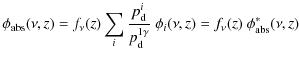
profile. As explained earlier (Chluba & Sunyaev 2009c), in the normal ``1+1'' photon language the Lyman ![]() line-emission and absorption terms can be cast into the form
line-emission and absorption terms can be cast into the form
![\begin{displaymath}%
\frac{1}{c}\left.\frac{{\rm d} N_{\nu}}{{\rm d} t}\right\ve...
...amma}_{\rm d}~h\nu_{\rm 21}~B_{12}~ N_{1\rm s}~N_{\nu}\right].
\end{displaymath}](/articles/aa/full_html/2010/04/aa12263-09/img75.png)
Here
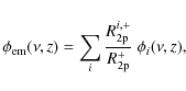
2.1.1 Introducing the thermodynamic correction factor
As mentioned in the introduction, in the form of Eq. (1), this equation does not exactly
conserve a blackbody spectrum in the case of full thermodynamic
equilibrium. Knowing the ``1+1'' photon line emission term and
using the detailed balance principle one can obtain the thermodynamic correction factor![]()
![\begin{displaymath}%
f_\nu(z)=\frac{\nu_{21}^2}{\nu^2}~{\rm e}^{h[\nu-\nu_{21}]/kT_{\gamma}(z)},
\end{displaymath}](/articles/aa/full_html/2010/04/aa12263-09/img83.png)
which is necessary to avoid this problem.
This factor was already introduced in Chluba & Sunyaev (2009c). Inserting it into Eq. (1), we then have
![\begin{displaymath}%
\frac{1}{c}\left.\frac{{\rm d} N_{\nu}}{{\rm d} t}\right\ve...
...{\rm d}~h\nu_{\rm 21}~B_{12}~ N_{1\rm s}~f_\nu~N_{\nu}\right].
\end{displaymath}](/articles/aa/full_html/2010/04/aa12263-09/img84.png)
In the standard ``1+1'' photon formulation,
2.1.2 Including the corrections due to the profiles of the different decay channels
As a next step, we take the differences between the line profiles of
the different absorption and emission channels into account. In
Eq. (3), one can see that there is no distinction between the different routes the electron took before or after entering the
![]() transition.
However, as mentioned in the introduction, the line-emission profiles
depend on how the fresh electron reached the 2p-state via channels
other than the Lyman
transition.
However, as mentioned in the introduction, the line-emission profiles
depend on how the fresh electron reached the 2p-state via channels
other than the Lyman ![]() transition.
transition.
To distinguish between the different possibilities (e.g.,
![]() ), one should allow for profiles,
), one should allow for profiles,
![]() ,
that depend on the channel i. The partial rate at which electrons enter the 2p-state will also depend on i, leading to the replacement
,
that depend on the channel i. The partial rate at which electrons enter the 2p-state will also depend on i, leading to the replacement
![]() with
with
![]() ,
where the sum runs over all possible ``1+1'' photon channels by means of which the number of Lyman
,
where the sum runs over all possible ``1+1'' photon channels by means of which the number of Lyman ![]() photons
can be affected. Furthermore, the probability of electrons being
absorbed will become channel-dependent, so that
photons
can be affected. Furthermore, the probability of electrons being
absorbed will become channel-dependent, so that
![]() with
with
![]() .
.
Here it is important that
![]() and
and
![]() both depend only on time but not on frequency. This is because
microscopically it is assumed that the absorption process leads to a
complete redistribution over the profile
both depend only on time but not on frequency. This is because
microscopically it is assumed that the absorption process leads to a
complete redistribution over the profile
![]() .
Then it is also clear that the factor
.
Then it is also clear that the factor ![]() should be independent of the channel, since otherwise detailed balance for each process cannot be achieved.
should be independent of the channel, since otherwise detailed balance for each process cannot be achieved.
With this in mind, it is clear that the more general form of Eq. (3) should read
![\begin{displaymath}%
\frac{1}{c}\left.\frac{{\rm d} N_{\nu}}{{\rm d} t}\right\ve...
...{\rm d}~h\nu_{\rm 21} B_{12}~ N_{1\rm s}~f_\nu~N_{\nu}\right].
\end{displaymath}](/articles/aa/full_html/2010/04/aa12263-09/img94.png)
In Appendix A, we argue that both
We note that because in two-photon transitions
![]() from n>3 also photons connected with the other Lyman series are emitted, Eq. (4)
can in principle be used to describe the simultaneous evolution of all
Lyman series photons. Similarly, one can account for the two-photon
corrections due to transitions from the continuum
from n>3 also photons connected with the other Lyman series are emitted, Eq. (4)
can in principle be used to describe the simultaneous evolution of all
Lyman series photons. Similarly, one can account for the two-photon
corrections due to transitions from the continuum
![]() ,
by simultaneously including the Lyman continuum and all other
continuua. However, in this case one can no longer clearly
distinguish between the different Lyman series. The equation will also
simultaneously describe the process of Ly-n feedback (Chluba & Sunyaev 2007),
and in addition account for its exact time-dependence.
To avoid these complications, below we first take into account
only the two-photon corrections for the 3s-1s and 3d-1s channel,
but leave the others unchanged. In this case, it is possible to
directly compare the results with those of the normal Lyman
,
by simultaneously including the Lyman continuum and all other
continuua. However, in this case one can no longer clearly
distinguish between the different Lyman series. The equation will also
simultaneously describe the process of Ly-n feedback (Chluba & Sunyaev 2007),
and in addition account for its exact time-dependence.
To avoid these complications, below we first take into account
only the two-photon corrections for the 3s-1s and 3d-1s channel,
but leave the others unchanged. In this case, it is possible to
directly compare the results with those of the normal Lyman ![]() problem. In Sect. 7, we briefly discuss the expected effect of this approximation, but leave a detailed analysis to another paper.
problem. In Sect. 7, we briefly discuss the expected effect of this approximation, but leave a detailed analysis to another paper.
2.2 Solution of the transfer equation
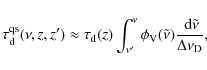
For a given ionization history, the solution of Eq. (4) in the expanding Unverse can be readily found, using the procedure described in Chluba & Sunyaev (2009c). If we introduce the effective absorption optical depth as
![$\displaystyle \tau_{\rm abs}(\nu, z', z) =\int_{z}^{z'} p^{1\gamma}_{\rm d}~
\f...
...s}}{H (1+\tilde{z})}~\phi_{\rm abs}(x[1+\tilde{z}], \tilde{z}){~\rm d}\tilde{z}$](/articles/aa/full_html/2010/04/aa12263-09/img97.png)
with
then Eq. (4) takes the simple form

where
![]() is only redshift-dependent.
is only redshift-dependent.
The solution of this equation in the expanding Universe can be directly given (see Chluba & Sunyaev 2009c)
![\begin{displaymath}%
\Delta N^{\rm asym}_{\nu}(z) =[N_{\rm em}(z)-N^{\rm pl}_{\nu_{21}}]\times F(\nu, z).
\end{displaymath}](/articles/aa/full_html/2010/04/aa12263-09/img106.png)
Here the function


where
2.3 Number of absorbed photons and the effective Lyman
escape probability
With the solution given in Eq. (8), one can directly compute the number of absorbed photons. For this, we define the mean of
![]() over the absorption profile
over the absorption profile

where we have set
Here P will later be interpreted as the main part of the effective escape probability (see Sects. 2.3.2 and 5).
As for
![]() ,
one can also define
,
one can also define
so that with the transfer equation given in Eq. (7), it follows that

where

where
2.3.1 Range of integration over the profiles
In the above derivation, we have not specified the range of
integration. Since the 3s and 3d two-photon profile include both
the Balmer ![]() and Lyman
and Lyman ![]() photons, by carrying out the integrals over the frequency interval
photons, by carrying out the integrals over the frequency interval
![]() ,
one would count
,
one would count ![]() per transition.
To avoid this problem, we can simply restrict the range of integration to
per transition.
To avoid this problem, we can simply restrict the range of integration to
![]() ,
but leave all the other definitions unaltered. Since
,
but leave all the other definitions unaltered. Since
![]() is far away from the Lyman
is far away from the Lyman ![]() resonance, this does not lead to any significant problem regarding the normalization of the normal Voigt function
resonance, this does not lead to any significant problem regarding the normalization of the normal Voigt function![]() .
In addition, for the quasi-stationary approximation the
contribution to the value of the escape probability from this region
are completely negligible. Therefore, this restriction does not lead to
any bias in the result, but does simplify the numerical integration
significantly.
.
In addition, for the quasi-stationary approximation the
contribution to the value of the escape probability from this region
are completely negligible. Therefore, this restriction does not lead to
any bias in the result, but does simplify the numerical integration
significantly.
2.3.2 Relating the corrections to the spectral distortion, to the corrections in the effective escape probability
We now want to understand how differences in ![]() and
and
![]() relate
to corrections in the effective escape probability. We first wish to
emphasize that in the normal ``1+1'' photon picture, based on the
assumption of quasi-stationarity and the no line-scattering
approximation, following the derivation of the previous section one
would find (Chluba & Sunyaev 2009c)
relate
to corrections in the effective escape probability. We first wish to
emphasize that in the normal ``1+1'' photon picture, based on the
assumption of quasi-stationarity and the no line-scattering
approximation, following the derivation of the previous section one
would find (Chluba & Sunyaev 2009c)
![\begin{displaymath}%
\left.\frac{{\rm d} N^{\rm d}_{\gamma}}{{\rm d} t}\right\ve...
...{12}~N_{\rm 1s}~
P_{\rm d}~[N_{\rm em}-N^{\rm pl}_{\nu_{21}}],
\end{displaymath}](/articles/aa/full_html/2010/04/aa12263-09/img149.png)
where
It is clear that
![]() represents the effective change in the total number density of photons involved in the Lyman
represents the effective change in the total number density of photons involved in the Lyman ![]() evolution over a short time interval
evolution over a short time interval ![]() ,
and hence is directly related to the change in the total number of
electrons that settle into the ground state by means of the Lyman
,
and hence is directly related to the change in the total number of
electrons that settle into the ground state by means of the Lyman ![]() channel. By comparing
channel. By comparing ![]() with
with
![]() ,
as defined by Eq. (12b),
one can therefore deduce the required effective correction to the
Sobolev escape probability that is normally used in the formulation of
the recombination problem. Following the arguments of Chluba & Sunyaev (2009c), this correction should be given by
,
as defined by Eq. (12b),
one can therefore deduce the required effective correction to the
Sobolev escape probability that is normally used in the formulation of
the recombination problem. Following the arguments of Chluba & Sunyaev (2009c), this correction should be given by

where
3 Main sources of corrections to the Lyman
spectral distortion
Using the solution given in Eq. (8)
one can already identify the main sources of corrections to the photon
distribution in comparison with the quasi-stationary approximation.
These can be devided into those acting as a time and
frequency-dependent emissivity, which is characterized by
![]() ,
and those just affecting the absorption optical depth,
,
and those just affecting the absorption optical depth,
![]() .
Below we explain how the two-photon aspect of the problem enters here, and which effects are expected. In Sects. 4 and 5, we discuss the corrections to the Lyman
.
Below we explain how the two-photon aspect of the problem enters here, and which effects are expected. In Sects. 4 and 5, we discuss the corrections to the Lyman ![]() spectral
distortion and the effective escape probability in comparison with the
standard ``1+1'' photon formulation, in more detail.
spectral
distortion and the effective escape probability in comparison with the
standard ``1+1'' photon formulation, in more detail.
![\begin{figure}
\par\includegraphics[width=8.5cm,clip]{eps/12263f01.eps}
\end{figure}](/articles/aa/full_html/2010/04/aa12263-09/img159.png)
|
Figure 1:
The death probabilities for different Lyman |
| Open with DEXTER | |
![\begin{figure}
\par\includegraphics[width=8.5cm,clip]{eps/12263f02.eps}\hspace*{4mm}
\includegraphics[width=8.5cm,clip]{eps/12263f03.eps}
\end{figure}](/articles/aa/full_html/2010/04/aa12263-09/img161.png)
|
Figure 2:
Different line profiles in the vicinity of the Lyman |
| Open with DEXTER | |
3.1 Relative importance of the different Lyman
absorption channels
Before studying at the solution of the transfer equation in more
detail, it is important to understand which channels on average
contribute the most to the absorption of Lyman ![]() photons. In Fig. 1, we present the partial death probabilities for different channels, as defined in Appendix A. At all considered redshifts, more than
photons. In Fig. 1, we present the partial death probabilities for different channels, as defined in Appendix A. At all considered redshifts, more than
![]() of the absorbed Lyman
of the absorbed Lyman ![]() photons disappear from the photon distribution in 1s-3d two-photon transitions. In contrast, only about
photons disappear from the photon distribution in 1s-3d two-photon transitions. In contrast, only about ![]() of all transitions end in the 3s-state. This is because the ratio of the 2p-3s to 2p-3d transition rates is about
of all transitions end in the 3s-state. This is because the ratio of the 2p-3s to 2p-3d transition rates is about
![]() .
In general, one can also see that the 1s-nd channels are more important than the 1s-ns channels,
and that the contributions of 1s-3s and 1s-4d two-photon channels are
comparable, whereas at high redshift the 1s-4d channels contributes
slightly more (
.
In general, one can also see that the 1s-nd channels are more important than the 1s-ns channels,
and that the contributions of 1s-3s and 1s-4d two-photon channels are
comparable, whereas at high redshift the 1s-4d channels contributes
slightly more (![]() versus
versus ![]() ). However, fewer than
). However, fewer than
![]() of photons are directly absorbed by the continuum.
of photons are directly absorbed by the continuum.
Assuming that the final modification to the ionization history is
![]() ,
when only
including the two-photon aspects for the 3d-1s channel, then the
above numbers suggest that: (i) the additional correction is
expected to be similar to
,
when only
including the two-photon aspects for the 3d-1s channel, then the
above numbers suggest that: (i) the additional correction is
expected to be similar to
![]() ,
when taking also the two-photon character of the 1s-3s, 1s-4d, and
1s-5d channels into account; (ii) neglecting the two-photon
character of the transition to the continuum should lead to an
uncertainty of
,
when taking also the two-photon character of the 1s-3s, 1s-4d, and
1s-5d channels into account; (ii) neglecting the two-photon
character of the transition to the continuum should lead to an
uncertainty of
![]() .
These simple conclusions seem to be in good agreement with the computations of Hirata (2008).
This also justifies why here as a first step we consider only the
two-photon corrections to the 3s-1s and 3d-1s channel. However, we
plan to take the other two-photon corrections into account in a
future paper.
.
These simple conclusions seem to be in good agreement with the computations of Hirata (2008).
This also justifies why here as a first step we consider only the
two-photon corrections to the 3s-1s and 3d-1s channel. However, we
plan to take the other two-photon corrections into account in a
future paper.
3.2 Effective Lyman
emission and absorption profile
As we have seen in the previous section, the main channel for Lyman ![]() absorption is related to the 1s-3d two-photon transition. This implies that the effective absorption profile,
absorption is related to the 1s-3d two-photon transition. This implies that the effective absorption profile,
![]() ,
is very close to that following from the 3d-1s channel alone. In Fig. 2, we illustrate the spectral dependence of different line profiles in the vicinity of the Lyman
,
is very close to that following from the 3d-1s channel alone. In Fig. 2, we illustrate the spectral dependence of different line profiles in the vicinity of the Lyman ![]() resonance at redshift z=1300. For comparison, we also show the Voigt profile,
resonance at redshift z=1300. For comparison, we also show the Voigt profile,
![]() (see Appendix D). One can clearly see the asymmetry of the two-photon profiles around the Lyman
(see Appendix D). One can clearly see the asymmetry of the two-photon profiles around the Lyman ![]() line center and the deviations from the Lorentzian shape in the distant damping wings.
line center and the deviations from the Lorentzian shape in the distant damping wings.
In the right panel, we also show the effective emission profile,
![]() ,
for the 3-shell atom, as defined by Eq. (6).
In the computations, we included only the 3s and
3d two-photon profiles, but assumed that in the continuum channel
(
,
for the 3-shell atom, as defined by Eq. (6).
In the computations, we included only the 3s and
3d two-photon profiles, but assumed that in the continuum channel
(
![]() ) photons
are emitted according to the normal Voigt profile. As one can
see, the effective emission profile is indeed very close to the 3d-1s
two-photon profile, including stimulated emission. Only at
) photons
are emitted according to the normal Voigt profile. As one can
see, the effective emission profile is indeed very close to the 3d-1s
two-photon profile, including stimulated emission. Only at
![]() can one see the small Lorentzian contribution from the continuum channel. Close to
can one see the small Lorentzian contribution from the continuum channel. Close to ![]() ,
one can also see the small admixture of the 3s-1s two-photon
profile. As can be deduced from the left panel in Fig. 2, at
,
one can also see the small admixture of the 3s-1s two-photon
profile. As can be deduced from the left panel in Fig. 2, at
![]() the stimulated 3s-1s two-photon profile is about
the stimulated 3s-1s two-photon profile is about ![]() times
larger than the 3d-1s two-photon profile. With appropriate
renormalization, one can also obtain this factor using the
approximation given by Eq. (C.3). Although
times
larger than the 3d-1s two-photon profile. With appropriate
renormalization, one can also obtain this factor using the
approximation given by Eq. (C.3). Although
![]() ,
because of this factor at
,
because of this factor at
![]() the 3s channel adds about
the 3s channel adds about
![]() ,
or
,
or
![]() to the effective emission profile.
to the effective emission profile.
![\begin{figure}
\par\includegraphics[width=8cm,clip]{eps/12263f04.eps}\vspace*{1....
...}\vspace*{1.5mm}
\includegraphics[width=8cm,clip]{eps/12263f06.eps}
\end{figure}](/articles/aa/full_html/2010/04/aa12263-09/img177.png)
|
Figure 3:
Modifications in the absorption optical depth
|
| Open with DEXTER | |
3.3 Time and frequency dependence of the absorption optical depth
In the definition of ![]() ,
i.e., Eq. (8b), the function
,
i.e., Eq. (8b), the function
![]() accounts for the frequency and time dependence of the emission process. For
accounts for the frequency and time dependence of the emission process. For
![]() ,
the shape of the solution for the spectral distortion depends only on the absorption optical depth,
,
the shape of the solution for the spectral distortion depends only on the absorption optical depth,
![]() ,
as defined by Eq. (5a).
In this case, one can write directly
,
as defined by Eq. (5a).
In this case, one can write directly

Separating this part of the solution is very useful for numerical purposes. However, as we see in Sect. 3.4.2, F0 does not describe the main behavior of the spectral distortion when including the thermodynamic correction factor
3.3.1 Purely time-dependent correction to

If we neglect the two-photon corrections to the 3s and 3d profiles (
![]() )
and define
)
and define
![]() then we can look at the purely time-dependent correction to
then we can look at the purely time-dependent correction to
![]() .
As explained earlier (Chluba & Sunyaev 2009c), the dependencies of
.
As explained earlier (Chluba & Sunyaev 2009c), the dependencies of ![]() ,
,
![]() ,
and H
on redshift lead to deviations in the solution for the spectral
distortion from the quasi-stationary case. Here the most important
aspects are that, depending on the emission redshift, the total
absorption optical depth until the time of observation (here z), is effectively lower (for
,
and H
on redshift lead to deviations in the solution for the spectral
distortion from the quasi-stationary case. Here the most important
aspects are that, depending on the emission redshift, the total
absorption optical depth until the time of observation (here z), is effectively lower (for
![]() ), or greater (for
), or greater (for
![]() )
than in the quasi-stationary case. In addition, the deviation from
the quasi-stationary case depends on the initial frequency of the
considered photon, since close to the line center photons travel a much
shorter distance before becoming absorbed than in the very distant
wings, implying that time-dependent corrections are only important to
photons that are emitted outside the Doppler core (for more details see
Chluba & Sunyaev 2009c).
)
than in the quasi-stationary case. In addition, the deviation from
the quasi-stationary case depends on the initial frequency of the
considered photon, since close to the line center photons travel a much
shorter distance before becoming absorbed than in the very distant
wings, implying that time-dependent corrections are only important to
photons that are emitted outside the Doppler core (for more details see
Chluba & Sunyaev 2009c).
In Fig. 3, we illustrate these effects on
![]() for emission redshift z=1100. We show the optical depth as a function of the initial frequency for different
for emission redshift z=1100. We show the optical depth as a function of the initial frequency for different ![]() .
In the upper panel, we give the results for the case under
discussion here (solid line). For comparison, we show the values
of the optical depth using the normal quasi-stationary optical depth
(dashed lines) for which one has
.
In the upper panel, we give the results for the case under
discussion here (solid line). For comparison, we show the values
of the optical depth using the normal quasi-stationary optical depth
(dashed lines) for which one has
where
For very small
![]() ,
one expects no significant difference between the full numerical result for
,
one expects no significant difference between the full numerical result for
![]() and this approximation. However, looking at the cases
and this approximation. However, looking at the cases
![]() ,
10-4, and 10-3
one can see that even then there is a small difference in the distant
red and blue wings of the line. This is not because of
time-dependent corrections but because, as usual, in Eq. (16) we neglected the factor
,
10-4, and 10-3
one can see that even then there is a small difference in the distant
red and blue wings of the line. This is not because of
time-dependent corrections but because, as usual, in Eq. (16) we neglected the factor
![]() ,
which appears in the definition of
,
which appears in the definition of
![]() ,
leading to
,
leading to
![]() on the red, and
on the red, and
![]() on the blue side of the resonance.
on the blue side of the resonance.
For the cases
![]() and 0.1, we start to see the corrections due to the time-dependence. For
and 0.1, we start to see the corrections due to the time-dependence. For
![]() in both wings, we find that
in both wings, we find that
![]() .
This is because the photons were released at
.
This is because the photons were released at ![]() ,
so that
,
so that
![]() decreases while the photons travel (Chluba & Sunyaev 2009c). This means that the integral over different redshifts
decreases while the photons travel (Chluba & Sunyaev 2009c). This means that the integral over different redshifts
![]() cannot reach the full value for
cannot reach the full value for
![]() .
We note that comparing with the value
.
We note that comparing with the value
![]() at the absorption redshift
at the absorption redshift
![]() ,
one finds that
,
one finds that
![]() following a similar argument. Usually this is the comparison made when talking about the escape probability at redshift z, so that the role of z and z' is simply interchanged.
following a similar argument. Usually this is the comparison made when talking about the escape probability at redshift z, so that the role of z and z' is simply interchanged.
In the distant wings of the line profile, the difference due to the time-dependence is not very visible for
![]() (the changes should be
(the changes should be
![]() ). However, one can see it in the region
). However, one can see it in the region
![]() .
There it is clear that the emitted photons will reach the Doppler core over a period that is shorter than the chosen
.
There it is clear that the emitted photons will reach the Doppler core over a period that is shorter than the chosen
![]() .
For the case
.
For the case
![]() ,
this region is
,
this region is
![]() .
Depending on how far the photon initially was emitted from the Doppler core the time that it will travel before reaching
.
Depending on how far the photon initially was emitted from the Doppler core the time that it will travel before reaching
![]() will grow with increasing
will grow with increasing
![]() .
This implies that at a redshift
.
This implies that at a redshift
![]() of Doppler core crossing, we have
of Doppler core crossing, we have
![]() ,
leading to the slope seen in the regions
,
leading to the slope seen in the regions
![]() .
.
In the final result, we note the time-dependent correction to
![]() is not so important, only leading to modifications in the escape probability by
is not so important, only leading to modifications in the escape probability by
![]() .
The time-dependence of
.
The time-dependence of
![]() is far more relevant (see Sect. 5 for more details).
is far more relevant (see Sect. 5 for more details).
3.3.2 Effect of thermodynamic correction factor on
If we now include the thermodynamic correction factor ![]() ,
as given by Eq. (2), in the computation of
,
as given by Eq. (2), in the computation of
![]() ,
then it is clear that for photons appearing at a given time on the red side of the Lyman
,
then it is clear that for photons appearing at a given time on the red side of the Lyman ![]() resonance, the total absorption optical depth over a fixed redshift interval will be lower than in the standard approach, independent of the emission redshift. Since
resonance, the total absorption optical depth over a fixed redshift interval will be lower than in the standard approach, independent of the emission redshift. Since
![]() ,
one has
,
one has
![]() .
Because of the exponential dependence of
.
Because of the exponential dependence of ![]() on the distance to the line center, this implies that at
on the distance to the line center, this implies that at
![]() photons
even directly escape, without any further reabsorption. This is in
stark contrast to the standard approximation (
photons
even directly escape, without any further reabsorption. This is in
stark contrast to the standard approximation (![]() )
for which even at distances
)
for which even at distances
![]() ,
some small fraction of photons (comparable to 10-3 at
,
some small fraction of photons (comparable to 10-3 at
![]() )
still disappears. We illustrate this behavior in the central panel of Fig. 3, where at large distances on the red side of the resonance, the value of
)
still disappears. We illustrate this behavior in the central panel of Fig. 3, where at large distances on the red side of the resonance, the value of
![]() is many orders of magnitude smaller than in the quasi-stationary approximation.
As we see below (e.g., Sect. 5.1), the thermodynamic factor leads to the largest correction discussed in this paper, and it is this red wing suppression of the absorption cross-section that contributes most.
is many orders of magnitude smaller than in the quasi-stationary approximation.
As we see below (e.g., Sect. 5.1), the thermodynamic factor leads to the largest correction discussed in this paper, and it is this red wing suppression of the absorption cross-section that contributes most.
As mentioned in Sect. 2.1.1,
this behavior reflects physically that the photon that enables the
2p-electron to reach the 3s and 3d is drawn from the ambient
CMB radiation field. For photons on the red side of the Lyman ![]() resonance (
resonance (
![]() ), another photon with
), another photon with
![]() is necessary for a 1s electron to reach the third shell. Since during H I recombination the Balmer
is necessary for a 1s electron to reach the third shell. Since during H I recombination the Balmer ![]() line is already in the Wien tail of the CMB, this means that relative to the Balmer
line is already in the Wien tail of the CMB, this means that relative to the Balmer ![]() line center the amount of photons at
line center the amount of photons at
![]() is exponentially
smaller, depending on how large the detuning is. Denoting the
frequency of the second photon (absorbed close to the Balmer
is exponentially
smaller, depending on how large the detuning is. Denoting the
frequency of the second photon (absorbed close to the Balmer ![]() resonance) with
resonance) with
![]() ,
by taking the ratio of the photon occupation numbers, i.e.,
,
by taking the ratio of the photon occupation numbers, i.e.,
![]() ,
we again can confirm the exponential behavior of
,
we again can confirm the exponential behavior of ![]() .
We note that the same factor appears when considering two-photon transitions towards higher levels with n>3
or the continuum. It is a result of thermodynamic requirements,
which should be independent of the considered process, as long as the
second photon is drawn from the CMB blackbody.
.
We note that the same factor appears when considering two-photon transitions towards higher levels with n>3
or the continuum. It is a result of thermodynamic requirements,
which should be independent of the considered process, as long as the
second photon is drawn from the CMB blackbody.
On the other hand, for photons released on the blue side of the Lyman ![]() line, the total absorption optical depth is larger than in the standard approximation (see Fig. 3 central panel for illustration). Because of the exponential dependence of
line, the total absorption optical depth is larger than in the standard approximation (see Fig. 3 central panel for illustration). Because of the exponential dependence of ![]() on frequency, for
on frequency, for
![]() this even leads to an arbitrarily
large absorption optical depth in the very distant blue wing. Again
this behavior can be understood by assuming that the second photon is
drawn from the CMB blackbody. However, there are now exponentially
more photons available than at the Balmer
this even leads to an arbitrarily
large absorption optical depth in the very distant blue wing. Again
this behavior can be understood by assuming that the second photon is
drawn from the CMB blackbody. However, there are now exponentially
more photons available than at the Balmer ![]() line center.
line center.
This very strong increase in the absorption optical depth implies that photons are basically reabsorbed quasi-instantaneously, so that at
![]() the usual quasi-stationary approximation for the computation of
the usual quasi-stationary approximation for the computation of
![]() should be possible, as inside the Doppler core. In this case, one therefore has
should be possible, as inside the Doppler core. In this case, one therefore has


where
For
![]() ,
,
![]() and assuming that
and assuming that
![]() ,
one has
,
one has

With this equation, it is possible to estimate the position on the blue side of the Lyman
3.3.3 Effect of line absorption profile on
It is clear that the shape of the absorption profile also
has an effect on the frequency dependence of the absorption optical
depth. As we explained in Sect. 3.2, the effective absorption profile,
![]() is very close to the two-photon emission profile of the 3d-level (see Fig. 2). For simplicity assuming that
is very close to the two-photon emission profile of the 3d-level (see Fig. 2). For simplicity assuming that
![]() ,
it is clear that at
,
it is clear that at
![]() ,
no photons can be absorbed in the Lyman
,
no photons can be absorbed in the Lyman ![]() transition, since there
transition, since there
![]() .
This is in stark contrast to the case of a normal Voigt profile,
for which in principle some photons can be absorbed at arbitrarily high
frequencies. Considering photons that reach the frequency interval
.
This is in stark contrast to the case of a normal Voigt profile,
for which in principle some photons can be absorbed at arbitrarily high
frequencies. Considering photons that reach the frequency interval
![]() ,
since in that region
,
since in that region
![]() (see Fig. 2), the contribution to the total absorption optical depth coming from this region is smaller than in the standard ``1+1'' photon formulation. Similarly, at
(see Fig. 2), the contribution to the total absorption optical depth coming from this region is smaller than in the standard ``1+1'' photon formulation. Similarly, at
![]() the contribution to the total absorption optical depth becomes larger than in the standard case, because there
the contribution to the total absorption optical depth becomes larger than in the standard case, because there
![]() .
.
In Fig. 3, lower panel, we illustrate these effects on
![]() for the 3-shell hydrogen atom. However, here we used the full absorption profile,
for the 3-shell hydrogen atom. However, here we used the full absorption profile,
![]() ,
which at
,
which at
![]() has a small contribution from the Voigt profile used to model the continuum channel (
has a small contribution from the Voigt profile used to model the continuum channel (
![]() ). Therefore, the optical depth does not vanish at
). Therefore, the optical depth does not vanish at
![]() .
The additional differences to the values of the optical depth seen in Fig. 3
confirm the above statements. Comparing with the case for the
thermodynamic factor (central panel), it is clear that the
correction to
.
The additional differences to the values of the optical depth seen in Fig. 3
confirm the above statements. Comparing with the case for the
thermodynamic factor (central panel), it is clear that the
correction to
![]() due to the shape of the absorption profile is not as important.
due to the shape of the absorption profile is not as important.
One should also mention that setting
![]() and
and ![]() ,
we obtain the solution
,
we obtain the solution ![]() as given by Eq. (15). With the comments made above, one therefore expects a sharp decline in the value of
as given by Eq. (15). With the comments made above, one therefore expects a sharp decline in the value of ![]() for
for
![]() ,
since
,
since
![]() .
Numerically, we indeed find this behavior (see Sect.4).
.
Numerically, we indeed find this behavior (see Sect.4).
3.4 Time and frequency dependence of the effective emissivity
If we look at the definition of
![]() ,
i.e., Eq. (8c), and rewrite it as
,
i.e., Eq. (8c), and rewrite it as

![$\displaystyle \Theta^{\rm\phi}(z, z') =\frac{
\tilde{N}_{\rm em}(z')}
{\tilde{N...
...mes\left[\frac{\phi_{\rm em}(\nu',z')}{\phi^\ast_{\rm abs}(\nu',z')} -1\right],$](/articles/aa/full_html/2010/04/aa12263-09/img250.png)
we can clearly see that there are also three sources for the corrections to the effective emissivity. The first is related to the purely time-dependent correction (
3.4.1 Purely time-dependent correction to

For
![]() ,
we consider the purely time-dependent correction to the emission
coefficient. This correction has already been discussed in detail (Chluba & Sunyaev 2009c).
For quasi-stationary conditions, one would have
,
we consider the purely time-dependent correction to the emission
coefficient. This correction has already been discussed in detail (Chluba & Sunyaev 2009c).
For quasi-stationary conditions, one would have
![]() .
However, in the cosmological recombination problem
.
However, in the cosmological recombination problem
![]() most of the time. This leads to significant changes in the shape of the
spectral distortion at different redshifts, where at frequencies
most of the time. This leads to significant changes in the shape of the
spectral distortion at different redshifts, where at frequencies
![]() only
only
![]() is able to affect the distortion (Chluba & Sunyaev 2009c).
is able to affect the distortion (Chluba & Sunyaev 2009c).
3.4.2 Effect of thermodynamic correction factor in
If we only include the correction due to the thermodynamic factor ![]() then we have
then we have
![]() .
Since for
.
Since for
![]() ,
one has
,
one has
![]() ,
so that due to
,
so that due to ![]() one expects a similar effect on the shape of the distortion like from
one expects a similar effect on the shape of the distortion like from
![]() .
However, since
.
However, since
![]() at large detuning blueward of the line center, this correction can be very large. As mentioned in Sect. 3.3, from Eq. (15), one naively expects
at large detuning blueward of the line center, this correction can be very large. As mentioned in Sect. 3.3, from Eq. (15), one naively expects
![]() ,
but when including the factor
,
but when including the factor
![]() in
in
![]() instead we find that
instead we find that
![]() at large
at large
![]() .
.
To show this, we consider the solution for ![]() in this case, assuming that the quasi-stationary approximation (
in this case, assuming that the quasi-stationary approximation (
![]() and
and
![]() ,
between the emission and absorption redshift of the photons) is possible. Introducing the new variable
,
between the emission and absorption redshift of the photons) is possible. Introducing the new variable
![]() ,
and using
,
and using
![]() ,
where
,
where
![]() ,
one has
,
one has
![$\displaystyle \tau_{\rm d}(z)\int^{\chi_{\rm s}}_0{~\rm d}\chi'~{\rm e}^{-\tau_...
...i]}
=\frac{1-{\rm e}^{-\tau_{\rm d}~f_{\nu}[\chi_{\rm s}-\chi]}}{f_\nu(z)}\cdot$](/articles/aa/full_html/2010/04/aa12263-09/img264.png)
Since
![\begin{figure}
\par\mbox{\includegraphics[width=8.5cm,clip]{eps/12263f07.eps}\hspace*{4mm}
\includegraphics[width=8.5cm,clip]{eps/12263f08.eps} }\end{figure}](/articles/aa/full_html/2010/04/aa12263-09/img273.png)
|
Figure 4:
Difference in the Lyman |
| Open with DEXTER | |
3.4.3 Correction related to the quantum-mechanical asymmetry between emission and absorption profile
Since in general the admixture of the different transition channels to the emission and absorption profile is not identical, one does expect that
![]() .
We can also consider the difference between
.
We can also consider the difference between
![]() and
and
![]() ,
which will be given by
,
which will be given by
![\begin{displaymath}%
\Delta\phi(\nu)=\phi_{\rm abs}^\ast-\phi_{\rm em}
=
\sum_{...
...\frac{R^{i,+}_{\rm 2p}}{R^{+}_{\rm 2p}}\right]~ \phi_{i}(\nu).
\end{displaymath}](/articles/aa/full_html/2010/04/aa12263-09/img275.png)
Since in full thermodynamic equilibrium
4 Changes to the Lyman
spectral distortion
We show the detailed dependence of the resulting Lyman ![]() spectral distortion on the different corrections that are taken into
account. As explained above, three types of corrections are
considered here: (i) the time-dependent correction; (ii) the
thermodynamic correction factor
spectral distortion on the different corrections that are taken into
account. As explained above, three types of corrections are
considered here: (i) the time-dependent correction; (ii) the
thermodynamic correction factor ![]() ;
and (iii) the dependence on the detailed shape of the effective
line emission and absorption profiles. We start our discussion by
including these corrections first only in the computation of
;
and (iii) the dependence on the detailed shape of the effective
line emission and absorption profiles. We start our discussion by
including these corrections first only in the computation of
![]() but setting
but setting
![]() and
and
![]() (Sect. 4.1). In Sect. 4.2, we also allow for
(Sect. 4.1). In Sect. 4.2, we also allow for
![]() ,
but still set
,
but still set
![]() .
Finally, we also include the correction due to
.
Finally, we also include the correction due to
![]() (Sect. 4.3),
but this aspect of the problem is not found to be very important.
It should be possible to deduce all the other combinations from
these cases.
(Sect. 4.3),
but this aspect of the problem is not found to be very important.
It should be possible to deduce all the other combinations from
these cases.
4.1 Corrections related to
 for
for
 and
and

As a first case, we study the effect of different corrections to the absorption optical depth. For this we set
![]() and
and
![]() ,
meaning that in the emission coefficient
,
meaning that in the emission coefficient
![]() we
ignore both the purely time-dependent correction and the one related to
the shape of the profile. However, depending on the case considered, we
do allow for these corrections in the computation of
we
ignore both the purely time-dependent correction and the one related to
the shape of the profile. However, depending on the case considered, we
do allow for these corrections in the computation of
![]() .
In addition, we also discuss the effect of the thermodynamic correction factor,
.
In addition, we also discuss the effect of the thermodynamic correction factor, ![]() .
but here we include it in both
.
but here we include it in both
![]() and
and
![]() at the same time. As explained Sect. 3.4.2, if one were to include only
at the same time. As explained Sect. 3.4.2, if one were to include only ![]() for
for
![]() or
or
![]() separately,
the corresponding spectral distortion would not be physically very
meaningful. Therefore, we omit this case here.
separately,
the corresponding spectral distortion would not be physically very
meaningful. Therefore, we omit this case here.
![\begin{figure}
\par\mbox{\includegraphics[width=8cm,clip]{eps/12263f09.eps}\hspa...
...\hspace*{2mm}
\includegraphics[width=8cm,clip]{eps/12263f14.eps} }\end{figure}](/articles/aa/full_html/2010/04/aa12263-09/img282.png)
|
Figure 5:
Difference in the Lyman |
| Open with DEXTER | |
![\begin{figure}
\par\mbox{\includegraphics[width=8cm,clip]{eps/12263f15.eps}\hspa...
...\hspace*{2mm}
\includegraphics[width=8cm,clip]{eps/12263f20.eps} }\end{figure}](/articles/aa/full_html/2010/04/aa12263-09/img283.png)
|
Figure 6:
The Lyman |
| Open with DEXTER | |
4.1.1 Behavior very close to the line center
As an example, in Fig. 4 we show the Lyman ![]() spectral distortion at z=1100 in the close vicinity of the line center. We compare the results with the normal quasi-stationary solution (see Chluba & Sunyaev 2009c, for details)
spectral distortion at z=1100 in the close vicinity of the line center. We compare the results with the normal quasi-stationary solution (see Chluba & Sunyaev 2009c, for details)

with
If we also include the correction due to the shape of the absorption profile in the computation of
![]() (dashed-dotted curve), then we see that at
(dashed-dotted curve), then we see that at
![]() again the solution is practically identical to the solution in the
quasi-stationary case. Although one does expect some corrections to the
exact value of
again the solution is practically identical to the solution in the
quasi-stationary case. Although one does expect some corrections to the
exact value of
![]() at different frequencies below the line center
at different frequencies below the line center![]() , since
, since
![]() the effect on the shape of
the effect on the shape of
![]() will be exponentially small. However, looking at
will be exponentially small. However, looking at
![]() we can see that
we can see that
![]() ,
implying that
,
implying that
![]() .
Since blueward of the resonance
.
Since blueward of the resonance
![]() (see right panel of Fig. 2), it is already expected that the curve lies below that for the purely time-dependent correction (i.e.
(see right panel of Fig. 2), it is already expected that the curve lies below that for the purely time-dependent correction (i.e.
![]() ). However, it is found that the correction related to the shape of
). However, it is found that the correction related to the shape of
![]() overcompensates the purely time-dependent effect, which alone leads to
overcompensates the purely time-dependent effect, which alone leads to
![]() .
This shows that at the considered redshift the correction related
to the profile is slightly more important than the time-dependence.
.
This shows that at the considered redshift the correction related
to the profile is slightly more important than the time-dependence.
If we now only include the time-dependent correction and the effect of the thermodynamic correction factor (in both
![]() and
and
![]() ), then we obtain the dotted line. As expected from Eq. (20), very close to the Doppler core (
), then we obtain the dotted line. As expected from Eq. (20), very close to the Doppler core (
![]() )
one has
)
one has
![]() .
We also found this scaling at other redshifts (marginally visible in Fig. 5),
as long as the optical depth across the Doppler core is much
larger that unity, implying that the quasi-stationary approximation
is valid. However, outside this region the distortion differs
significantly from the previous cases. In particular, one finds
.
We also found this scaling at other redshifts (marginally visible in Fig. 5),
as long as the optical depth across the Doppler core is much
larger that unity, implying that the quasi-stationary approximation
is valid. However, outside this region the distortion differs
significantly from the previous cases. In particular, one finds
![]() at
at
![]() ,
which is the result of
,
which is the result of
![]() .
If we include the thermodynamic correction factor only in the computation of
.
If we include the thermodynamic correction factor only in the computation of
![]() ,
i.e., by setting
,
i.e., by setting
![]() ,
then we instead find
,
then we instead find
![]() .
.
It is also found that
![]() at
at
![]() .
This is in contrast to the result for
.
This is in contrast to the result for
![]() ,
given by Eq. (20),
for which we assume quasi-stationary conditions. This implies that in
the red damping wing deviations from the quasi-stationary assumption
become important.
,
given by Eq. (20),
for which we assume quasi-stationary conditions. This implies that in
the red damping wing deviations from the quasi-stationary assumption
become important.
In addition, if we include the correction due to the shape of the absorption profile, then we can see that at
![]() the
curve basically coincides with that from the previous case.
This again is expected since the tiny corrections to the value of a
very large optical depth will not lead to visible changes in
the
curve basically coincides with that from the previous case.
This again is expected since the tiny corrections to the value of a
very large optical depth will not lead to visible changes in ![]() .
In addition, at
.
In addition, at
![]() one can see that the differences to the previous case are about the
same as for the differences between the first two cases, owing to the
corrections being small and hence additive.
one can see that the differences to the previous case are about the
same as for the differences between the first two cases, owing to the
corrections being small and hence additive.
4.1.2 Behavior at intermediate and large distances from the line center
We now consider the corrections in a slightly wider range around the line center. In Fig. 5, we show the same cases as above, but now also varying the redshift.
As before, one can see that differences due to the shape of the absorption profile are negligible at
![]() .
Furthermore, on the blue side of the resonance the correction due to
the shape of the absorption profile is always negative, as also seen in
the previous paragraph.
.
Furthermore, on the blue side of the resonance the correction due to
the shape of the absorption profile is always negative, as also seen in
the previous paragraph.
Taking the differences between the curves for
![]() (first two lines), and those for
(first two lines), and those for
![]() (last two lines) one can also see that at z=1200 these are practically the same. However, for z=1000 and z=800, higher order terms already start to become important. For example, at
(last two lines) one can also see that at z=1200 these are practically the same. However, for z=1000 and z=800, higher order terms already start to become important. For example, at
![]() ,
the difference in the curves for
,
the difference in the curves for
![]() is
is
![]() ,
while it is about
,
while it is about
![]() for those with
for those with
![]() .
.
If we consider the distortion for an even wider range of frequencies (Fig. 6), then we can make several important observations. First, as expected from the discussion related to Eq. (20), in the limit
![]() for
for
![]() one finds that
one finds that
![]() ,
regardless of whether the normal Voigt profile was used or the effective absorption profile, given by Eq. (5a). However, for
,
regardless of whether the normal Voigt profile was used or the effective absorption profile, given by Eq. (5a). However, for
![]() the limit
the limit
![]() is
reached closer to the line center than for the effective absorption
profile. This is expected, since for the 3-shell atom the
effective absorption profile only has a small admixture of the Voigt
profile (because of the description of the route connecting to the
continuum). If
is
reached closer to the line center than for the effective absorption
profile. This is expected, since for the 3-shell atom the
effective absorption profile only has a small admixture of the Voigt
profile (because of the description of the route connecting to the
continuum). If
![]() ,
then the limit
,
then the limit
![]() would never be reached, simply because at
would never be reached, simply because at
![]() the contribution to
the contribution to
![]() would be zero. Reducing the admixture of the pure Voigt profile therefore moves the transition to
would be zero. Reducing the admixture of the pure Voigt profile therefore moves the transition to
![]() towards higher frequencies.
towards higher frequencies.
The second important observation is that in the frequency range
![]() on
the blue side of the resonance the correction due to the shape of the
absorption profile is far more important than both the pure
time-dependent correction to
on
the blue side of the resonance the correction due to the shape of the
absorption profile is far more important than both the pure
time-dependent correction to
![]() and the correction due to the
and the correction due to the
![]() factor in
factor in
![]() .
And finally, in the red wing the correction to the spectral distortion is dominated by the
.
And finally, in the red wing the correction to the spectral distortion is dominated by the
![]() scaling of
scaling of
![]() ,
although the correction is very small, in particular in comparison to that coming from
,
although the correction is very small, in particular in comparison to that coming from
![]() (see Sect. 4.2).
(see Sect. 4.2).
4.2 Corrections related to both
and
 but for
We now want to understand the effect of changes to the ionization
history and death probability on the effective emission rate. We
therefore allow
![]() ,
but still set
,
but still set
![]() .
We then again discuss different combinations of corrections, as in the
previous section. As we see, the corrections related to
.
We then again discuss different combinations of corrections, as in the
previous section. As we see, the corrections related to
![]() dominate at large distances on the red side of the resonance, while the
shape of the profile is most important to the spectral distortion on
the blue side of the resonance (see Fig. 6). In the vicinity of the resonance, basically all the correction factors are important.
dominate at large distances on the red side of the resonance, while the
shape of the profile is most important to the spectral distortion on
the blue side of the resonance (see Fig. 6). In the vicinity of the resonance, basically all the correction factors are important.
4.2.1 Behavior very close to the line center
In Fig. 4, we show the Lyman ![]() spectral distortion at z=1100 in the very close vicinity of the line center, now also including
spectral distortion at z=1100 in the very close vicinity of the line center, now also including
![]() .
If we first look at the curves for
.
If we first look at the curves for ![]() (dashed and dashed-dotted), then we can see that very close to the resonance (
(dashed and dashed-dotted), then we can see that very close to the resonance (
![]() )
the solution is unaffected by the inclusion of
)
the solution is unaffected by the inclusion of
![]() .
Due to the huge optical depth across the Doppler core (corresponding to
.
Due to the huge optical depth across the Doppler core (corresponding to
![]() ),
practically any time-dependent variation in the effective emission
coefficient is erased. However, moving towards the wings,
time-dependent aspects become important and in particular,
),
practically any time-dependent variation in the effective emission
coefficient is erased. However, moving towards the wings,
time-dependent aspects become important and in particular,
![]() at
at
![]() .
.
At the considered redshift, the difference from the case
![]() (see Fig. 4) is very small at
(see Fig. 4) is very small at
![]() .
Clearly, the correction due to the thermodynamic factor
.
Clearly, the correction due to the thermodynamic factor ![]() (dotted and solid lines) is dominant. However, at
(dotted and solid lines) is dominant. However, at
![]() the time-dependent changes in the effective emission coefficient lead to a correction that is as important as that due to
the time-dependent changes in the effective emission coefficient lead to a correction that is as important as that due to ![]() .
One can also see that all the corrections add roughly linearly.
We note that at
.
One can also see that all the corrections add roughly linearly.
We note that at
![]() the curves are not affected when accounting for corrections to the shape of the line profile.
the curves are not affected when accounting for corrections to the shape of the line profile.
4.2.2 Behavior at intermediate and large distances from the line center
Looking at the right column of Fig. 5, we can see that at
![]() the correction due to the inclusion of
the correction due to the inclusion of ![]() dominates at high redshift, while at
dominates at high redshift, while at
![]() the correction due to
the correction due to
![]() is already comparable, and clearly dominates at low redshift. In addition, at
is already comparable, and clearly dominates at low redshift. In addition, at
![]() one can see that at high redshift all the corrections practically add linearly, while for z=1000 and z=800 the correction due to the inclusion of
one can see that at high redshift all the corrections practically add linearly, while for z=1000 and z=800 the correction due to the inclusion of
![]() practically disappears when including the correct shape of the
effective absorption profile. When also including the thermodynamic
correction factor the large excess of photons seen for the case
practically disappears when including the correct shape of the
effective absorption profile. When also including the thermodynamic
correction factor the large excess of photons seen for the case ![]() and
and
![]() practically vanishes. This implies that the self-feedback effect at low redshifts reported elsewhere (Chluba & Sunyaev 2007)
is expected to disappear. As explained there, this unphysical
aspect of the solution in the ``1+1'' photon pictures is caused by
the Voigt profile in principle extending up to arbitrarily high
frequencies, so that photons emitted at
practically vanishes. This implies that the self-feedback effect at low redshifts reported elsewhere (Chluba & Sunyaev 2007)
is expected to disappear. As explained there, this unphysical
aspect of the solution in the ``1+1'' photon pictures is caused by
the Voigt profile in principle extending up to arbitrarily high
frequencies, so that photons emitted at
![]() in the very distant blue damping wing will still be able to reach the
line center at low redshift, strongly enhancing the photon occupation
number. However, when including the thermodynamic correction factor,
because of the exponential enhancement of the absorption optical depth
at large distances blueward of the resonance, these photons disappear
much before this.
Similarly, when including the shape of the effective emission profile
this excess of photons will never be produced in the first place, so
that from this region the residual correction due to
in the very distant blue damping wing will still be able to reach the
line center at low redshift, strongly enhancing the photon occupation
number. However, when including the thermodynamic correction factor,
because of the exponential enhancement of the absorption optical depth
at large distances blueward of the resonance, these photons disappear
much before this.
Similarly, when including the shape of the effective emission profile
this excess of photons will never be produced in the first place, so
that from this region the residual correction due to
![]() is much smaller.
is much smaller.
Looking at the spectral distortion for a very wide range of frequencies around the line center (Fig. 6), it is clear that at all redshifts the shape of the distortion is dominated by the correction due to
![]() for
for
![]() .
Both the thermodynamic factor and the shape of the absorption and
emission profile only lead to small additional modifications. The
largest correction is related to the 3d two-photon emission
profile being larger than the Voigt profile at
.
Both the thermodynamic factor and the shape of the absorption and
emission profile only lead to small additional modifications. The
largest correction is related to the 3d two-photon emission
profile being larger than the Voigt profile at
![]() ,
explaining the small addition of photons in comparison to the case
,
explaining the small addition of photons in comparison to the case
![]() seen close to the lowest frequencies shown in the figures. On the other
hand, at frequencies above the line center the correction due to the
shape of the line profile is clearly most important. In the line
center, all sources of correction contribute to changes to the
Lyman
seen close to the lowest frequencies shown in the figures. On the other
hand, at frequencies above the line center the correction due to the
shape of the line profile is clearly most important. In the line
center, all sources of correction contribute to changes to the
Lyman ![]() spectral distortion relative to the quasi-stationary solution.
spectral distortion relative to the quasi-stationary solution.
![\begin{figure}
\par\includegraphics[width=8.5cm,clip]{eps/12263f21.eps}
\end{figure}](/articles/aa/full_html/2010/04/aa12263-09/img320.png)
|
Figure 7:
Source of the asymmetry between the absorption and emission profiles,
|
| Open with DEXTER | |
4.3 Corrections related to
and
 including

We also considered cases for
![]() .
However, the correction was always extremely small. Therefore, we decided to omit the corresponding plots for
.
However, the correction was always extremely small. Therefore, we decided to omit the corresponding plots for ![]() .
As mentioned in Sect. 3.2, this is expected since the deviations of
.
As mentioned in Sect. 3.2, this is expected since the deviations of
![]() and
and
![]() from their equilibrium values is always very small in the relevant redshift range, so that
from their equilibrium values is always very small in the relevant redshift range, so that
![]() ,
and hence
,
and hence
![]() .
In Fig. 7, we explicitly show this fact. As an example, for the 3d-channel one can see that at
.
In Fig. 7, we explicitly show this fact. As an example, for the 3d-channel one can see that at
![]() one has
one has
![]() .
Therefore, one would expect corrections to the effective escape probability at the level of
.
Therefore, one would expect corrections to the effective escape probability at the level of
![]() ,
which is clearly negligible in the context of the CMB anisotropies.
We confirmed this statement numerically.
,
which is clearly negligible in the context of the CMB anisotropies.
We confirmed this statement numerically.
One should also mention that, although at low redshift the expected difference between emission and absorption profile increases, the value of the effective escape probability is dominated by the contribution from the Doppler core, where details of the profiles do not matter. In addition, corrections to the escape probability will not affect the ionization history significantly, so that here we do not discuss this point any further.
5 Changes to the effective escape probability
![\begin{figure}
\par\mbox{\includegraphics[width=8.5cm,clip]{eps/12263f22.eps}\includegraphics[width=8.7cm,clip]{eps/12263f23.eps} }\end{figure}](/articles/aa/full_html/2010/04/aa12263-09/img330.png)
|
Figure 8:
The functions
|
| Open with DEXTER | |
5.1 Effect of the thermodynamic correction factor
First we consider the normal Lyman ![]() transfer equation given in Eq. (1), but including the thermodynamic correction factor
transfer equation given in Eq. (1), but including the thermodynamic correction factor ![]() ,
to correct for the small imbalance between the emission and
absorption process in the line wings originating from the normal
``1+1'' photon formulation (see Sect. 2.1.1). In this case, one has
,
to correct for the small imbalance between the emission and
absorption process in the line wings originating from the normal
``1+1'' photon formulation (see Sect. 2.1.1). In this case, one has
![]() and hence
and hence
![]() ,
so that from Eq. (8b) one can find
,
so that from Eq. (8b) one can find


where
If one drops the factors related to ![]() in the definition of
in the definition of
![]() and also
and also
![]() ,
one obtains the purely time-dependent case,
,
one obtains the purely time-dependent case,
![]() ,
that was addressed earlier (Chluba & Sunyaev 2009c). However, here the term
,
that was addressed earlier (Chluba & Sunyaev 2009c). However, here the term
![]() is naturally given by the line center values of
is naturally given by the line center values of
![]() ,
which in the previous work had to be enforced for consistency with the
standard approximations (see comments in Sect. 3.4.1 of Chluba & Sunyaev 2009c).
,
which in the previous work had to be enforced for consistency with the
standard approximations (see comments in Sect. 3.4.1 of Chluba & Sunyaev 2009c).
To understand the role of ![]() in the final correction to
in the final correction to
![]() ,
in Eq. (12b), we first consider the term
,
in Eq. (12b), we first consider the term
![]() ,
in Eq. (12c). It is clear that for
,
in Eq. (12c). It is clear that for
![]() ,
one has
,
one has
![]() ,
since
,
since
![]()
![]()
![]() = 0. As we show below (Sect. 5.2.1),
= 0. As we show below (Sect. 5.2.1),
![]() when taking into account the effect of stimulated emission in the
blackbody radiation field, although, the contribution to the final
correction is found to be negligible.
when taking into account the effect of stimulated emission in the
blackbody radiation field, although, the contribution to the final
correction is found to be negligible.
If we now consider the definition of P, in Eq. (11b), then for the considered case we can rewrite this as
![\begin{displaymath}%
P^{\rm f} =\int\varphi_{\rm V}(\nu)~[1-\mathcal{F}^{\rm f}_\nu]{~\rm d}\nu,
\end{displaymath}](/articles/aa/full_html/2010/04/aa12263-09/img345.png)
where we have introduced the function

This representation allows us to see directly the expected differences compared to the standard quasi-stationary case, for which one has (
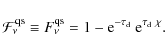
If instead of
![\begin{displaymath}%
\Delta P^{\rm f}_{\rm d} =P^{\rm f}-P_{\rm d}=-\int\phi_{\r...
...[\mathcal{F}^{\rm f}_\nu-\mathcal{F}^{\rm qs}_\nu]{~\rm d}\nu.
\end{displaymath}](/articles/aa/full_html/2010/04/aa12263-09/img350.png)
This expression shows that for the correction to the effective escape probability, it is not important how
5.1.1 Behavior of
 and the expected corrections to

In Fig. 8, as an example we show
![]() at redshift z=1000 (dotted lines). For comparison, we also show the purely time-dependent solution (dashed curves) for which
at redshift z=1000 (dotted lines). For comparison, we also show the purely time-dependent solution (dashed curves) for which
![]() .
We note that we include the correction terms in both
.
We note that we include the correction terms in both
![]() and
and
![]() .
.
If we focus on the behavior at
![]() ,
then we can see that although in the considered cases
,
then we can see that although in the considered cases
![]() (compare with Fig. 5, right column, case z=1000), for
(compare with Fig. 5, right column, case z=1000), for
![]() one has
one has
![]() .
This change in the sequence is related only to the factor
.
This change in the sequence is related only to the factor ![]() in the definition of
in the definition of
![]() ,
which appears because
,
which appears because
![]() in the escape integral, Eq. (11b). Instead of an additional negative contribution to the escape probability (
in the escape integral, Eq. (11b). Instead of an additional negative contribution to the escape probability (
![]() ), as would follow from the differences seen in
), as would follow from the differences seen in ![]() ,
when including the thermodynamic correction factor
,
when including the thermodynamic correction factor ![]() one therefore expects a positive
contribution from the considered spectral region. This effect becomes
even more apparent when looking at the very distant red wing, where
clearly
one therefore expects a positive
contribution from the considered spectral region. This effect becomes
even more apparent when looking at the very distant red wing, where
clearly
![]() ,
owing to the exponential cutoff introduced by
,
owing to the exponential cutoff introduced by ![]() .
The behavior shows that in the very distant red wing the excess Lyman
.
The behavior shows that in the very distant red wing the excess Lyman ![]() photons
no longer supports the flow of electrons toward higher levels and the
continuum. These photons only undergo line-scattering events, with tiny
shifts in the frequency caused by the Doppler motion of the atom, but
do not disappear anymore, and therefore effectively escape. As we
demonstrate below (Sects. 5.1.4 and 5.1.5), the main correction related to
photons
no longer supports the flow of electrons toward higher levels and the
continuum. These photons only undergo line-scattering events, with tiny
shifts in the frequency caused by the Doppler motion of the atom, but
do not disappear anymore, and therefore effectively escape. As we
demonstrate below (Sects. 5.1.4 and 5.1.5), the main correction related to ![]() is from the change in the absorption cross-section in the red wing of
the line profile. The true modifications to the spectral distortion due
to
is from the change in the absorption cross-section in the red wing of
the line profile. The true modifications to the spectral distortion due
to ![]() are not so important.
are not so important.
If we now look at the behavior in the range
![]() ,
we can see that the sequence
,
we can see that the sequence
![]() does not change when considering
does not change when considering
![]() ,
but
,
but
![]() becomes more similar to
becomes more similar to
![]() .
From the behavior at
.
From the behavior at
![]() and the strength of the changes there, one might have expected that at
and the strength of the changes there, one might have expected that at
![]() also
also
![]() ,
since
,
since
![]() is similar in both regions. However, at
is similar in both regions. However, at
![]() the spectral distortion
the spectral distortion ![]() is very steep, so that small changes
is very steep, so that small changes
![]() cannot affect the shape of
cannot affect the shape of
![]() so much in comparison to
so much in comparison to
![]() .
Only at much larger distances on the blue side of the resonance, where
.
Only at much larger distances on the blue side of the resonance, where ![]() again behaves exponentially, can one see that
again behaves exponentially, can one see that
![]() ,
although there
,
although there
![]() (compare with Fig. 6, right column, case z=1000). In comparison to the purely time-dependent correction for the range
(compare with Fig. 6, right column, case z=1000). In comparison to the purely time-dependent correction for the range
![]() ,
one therefore expects a slightly smaller (negative) correction to the total value of P,
while the contributions from very large distances in the blue wing
should be significantly larger than in the purely time-dependent case.
However, here it is important to mention that these very distant wing
contributions will always be very minor, since the Voigt profile
decreases like
,
one therefore expects a slightly smaller (negative) correction to the total value of P,
while the contributions from very large distances in the blue wing
should be significantly larger than in the purely time-dependent case.
However, here it is important to mention that these very distant wing
contributions will always be very minor, since the Voigt profile
decreases like
![]() (see Sect. 5.1.3).
(see Sect. 5.1.3).
Finally, in the central region
![]() ,
we can see that
,
we can see that
![]() .
This is because
.
This is because
![]() in these regions (see Sect. 4.1.1), so that
in these regions (see Sect. 4.1.1), so that
![]() to very high accuracy. Although the Lyman
to very high accuracy. Although the Lyman ![]() spectral distortions in the case
spectral distortions in the case
![]() and
and
![]() look rather different, this implies that a the correction factor
look rather different, this implies that a the correction factor ![]() does not lead to any real correction in the escape probability from
inside the Doppler core. Everything is well described by the
quasi-stationary assumption, for which the entire Doppler core reaches
thermodynamic equilibrium with the ambient radiation field, but now
also including the small additional variation in the photon
distribution over
does not lead to any real correction in the escape probability from
inside the Doppler core. Everything is well described by the
quasi-stationary assumption, for which the entire Doppler core reaches
thermodynamic equilibrium with the ambient radiation field, but now
also including the small additional variation in the photon
distribution over ![]() .
.
![\begin{figure}
\par\includegraphics[width=8.5cm,clip]{eps/12263f24.eps}
\end{figure}](/articles/aa/full_html/2010/04/aa12263-09/img378.png)
|
Figure 9: Relative difference in the effective escape probability with respect to the Sobolev escape probability: effect of the thermodynamic correction factor. |
| Open with DEXTER | |
5.1.2 Correction to the escape probability
In Fig. 9, we show the result for the effective escape probability and the effect of ![]() .
For comparison, we also show the result for the purely time-dependent
correction (dotted line), which was already discussed elsewhere (Chluba & Sunyaev 2009c).
At low redshifts, we indicate the increase in the amplitude of the
correction, which was attributed to the late self feedback of
Lyman
.
For comparison, we also show the result for the purely time-dependent
correction (dotted line), which was already discussed elsewhere (Chluba & Sunyaev 2009c).
At low redshifts, we indicate the increase in the amplitude of the
correction, which was attributed to the late self feedback of
Lyman ![]() photons for this case. For the other cases, we also point towards the
difference caused by the no-scattering approximation. It is
related to differences in
photons for this case. For the other cases, we also point towards the
difference caused by the no-scattering approximation. It is
related to differences in ![]() and
and ![]() ,
which close to the maximum of the Thomson visibility function at
,
which close to the maximum of the Thomson visibility function at
![]() are negligible, but become significant both at very low and very high redshifts (Chluba & Sunyaev 2009c).
However, the changes have no important effect on the free electron fraction.
are negligible, but become significant both at very low and very high redshifts (Chluba & Sunyaev 2009c).
However, the changes have no important effect on the free electron fraction.
When now including the thermodynamic correction factor in the
computation of the absorption optical depth and the effective emission
rate
![]() ,
but setting
,
but setting
![]() (dashed line), one can see that the correction to the escape probability becomes positive at all redshifts, with a maximum of
(dashed line), one can see that the correction to the escape probability becomes positive at all redshifts, with a maximum of
![]() at
at
![]() .
As we see in Sects. 5.1.4 and 5.1.5,
the bulk of this total correction originates from changes to the
absorption process on the red side of the resonance, where in this case
.
As we see in Sects. 5.1.4 and 5.1.5,
the bulk of this total correction originates from changes to the
absorption process on the red side of the resonance, where in this case
![]() (cf. Figs. 5 and 6, left column).
(cf. Figs. 5 and 6, left column).
When also including the variation in
![]() over time (solid line), the result changes significantly, shifting the maximum of the correction
over time (solid line), the result changes significantly, shifting the maximum of the correction
![]() to
to
![]() ,
but still leading to
,
but still leading to
![]() everywhere. However, especially the low redshift part is strongly modified, reducing the total correction by a factor of
everywhere. However, especially the low redshift part is strongly modified, reducing the total correction by a factor of ![]() at
at
![]() .
We also show the inferred correction related to
.
We also show the inferred correction related to
![]() alone,
which was obtained by taking the difference between the curves
labeled (I) and (II). The result shows that the final
correction close to the maximum of the Thomson visibility function has
important contributions from both
alone,
which was obtained by taking the difference between the curves
labeled (I) and (II). The result shows that the final
correction close to the maximum of the Thomson visibility function has
important contributions from both
![]() and the time-dependence of the problem.
and the time-dependence of the problem.
5.1.3 Effect at large distances blueward of the line center and the Lyman
self-feedback
The thermodynamic factor clearly strongly changes the behavior of the
correction to the effective escape probability. The purely
time-dependent correction is no longer dominant, and in particular the
thermodynamic factor removes the self feedback problem of Lyman ![]() at low redshifts, which was already realized to be an artifact of the standard ``1+1'' photon formulation (Chluba & Sunyaev 2009c). This is because when taking
at low redshifts, which was already realized to be an artifact of the standard ``1+1'' photon formulation (Chluba & Sunyaev 2009c). This is because when taking ![]() into account, exponentially fewer photons remain in the photon
distribution at large distances on the blue side of the resonance
(cf. Fig. 6 where
into account, exponentially fewer photons remain in the photon
distribution at large distances on the blue side of the resonance
(cf. Fig. 6 where
![]() at large
at large
![]() ). As explained in Sect. 3, every photon emitted at
). As explained in Sect. 3, every photon emitted at
![]() will be reabsorbed quasi-instantaneously. This is because of the
exponentially larger amount of CMB photons redward of the
Balmer
will be reabsorbed quasi-instantaneously. This is because of the
exponentially larger amount of CMB photons redward of the
Balmer ![]() line
compared to close to the line center, so that line absorption is
more effective. The main process for the death here is the
line
compared to close to the line center, so that line absorption is
more effective. The main process for the death here is the
![]() ,
where the last step is considered to lead to a complete redistribution, so that the absorbed Lyman
,
where the last step is considered to lead to a complete redistribution, so that the absorbed Lyman ![]() photon (
photon (
![]() )
will most likely reappear close to the line center. We note that in
this section we still do not include the two-photon corrections to the
shape of the absorption profile, but already now the two-photon
character of the process leads to this conclusion.
)
will most likely reappear close to the line center. We note that in
this section we still do not include the two-photon corrections to the
shape of the absorption profile, but already now the two-photon
character of the process leads to this conclusion.
However, one has to mention that basically all the photons
present at these large distances contribute to the escape integral.
This is because
![]() while
while
![]() ,
so that
,
so that
![]() (see Sect. 5.1.1 and Fig. 8). Therefore, in this case the very distant blue wing contribution to the value of
(see Sect. 5.1.1 and Fig. 8). Therefore, in this case the very distant blue wing contribution to the value of
![]() behaves like
behaves like

at
5.1.4 Contributions from the blue and red wing
Returning to the correction at higher redshifts (
![]() ), it was shown earlier, that there the Lyman
), it was shown earlier, that there the Lyman ![]() self feedback is not important (Chluba & Sunyaev 2009c). From Fig. 9, it is clear that both considered cases for the effect of
self feedback is not important (Chluba & Sunyaev 2009c). From Fig. 9, it is clear that both considered cases for the effect of ![]() imply that at a given redshift, effectively fewer photons support the
flow of electrons towards higher levels and the continuum than in the
quasi-stationary case, albeit that more photons are produced. The
latter statement can also be confirmed by looking at Fig. 6 and the amplitude of the Lyman
imply that at a given redshift, effectively fewer photons support the
flow of electrons towards higher levels and the continuum than in the
quasi-stationary case, albeit that more photons are produced. The
latter statement can also be confirmed by looking at Fig. 6 and the amplitude of the Lyman ![]() distortion in the distant red wing around its maximum. We note that these photons were already emitted at
distortion in the distant red wing around its maximum. We note that these photons were already emitted at
![]() .
.
However, from which part of the photon distribution do the main
correction to the escape probability at these redshifts come from?
Looking at Fig. 8, we can see that at
![]() ,
the function
,
the function
![]() is very similar to
is very similar to
![]() ,
which results in the purely time-dependent correction. Also at slightly larger distances (
,
which results in the purely time-dependent correction. Also at slightly larger distances (
![]() )
one still has
)
one still has
![]() .
Therefore, one does not expect very dramatic changes to the
contribution to the effective escape from this part of the Lyman
.
Therefore, one does not expect very dramatic changes to the
contribution to the effective escape from this part of the Lyman ![]() distortion compared to the purely time-dependent case.
distortion compared to the purely time-dependent case.
![\begin{figure}
\par\includegraphics[width=8.5cm,clip]{eps/12263f25.eps}\vspace*{1mm}
\includegraphics[width=8.5cm,clip]{eps/12263f26.eps}
\end{figure}](/articles/aa/full_html/2010/04/aa12263-09/img402.png)
|
Figure 10:
Difference between the effective escape probability and the Sobolev
escape probability: the effect of the thermodynamic correction factor
in the blue and red wing of the resonance. For the upper panel, we set
|
| Open with DEXTER | |
On the other hand, in the red wing one finds that
![]() ,
and at very large distances one even has
,
and at very large distances one even has
![]() .
Physically, this reflects that due to
.
Physically, this reflects that due to ![]() ,
the reabsorption process in the distant red wing is exponentially
suppressed, so that photons can escape more directly than in the
normal ``1+1'' photon formulation. This is now related to the
exponentially smaller amount of CMB photons blueward of the
Balmer
,
the reabsorption process in the distant red wing is exponentially
suppressed, so that photons can escape more directly than in the
normal ``1+1'' photon formulation. This is now related to the
exponentially smaller amount of CMB photons blueward of the
Balmer ![]() line, so that the main absorption channel
line, so that the main absorption channel
![]() becomes practically inactive at
becomes practically inactive at
![]() .
Therefore, it is the modifications to the red wing absorption
process from which one expects the largest effect in connection
with
.
Therefore, it is the modifications to the red wing absorption
process from which one expects the largest effect in connection
with ![]() at high redshifts, before the appearance of the self feedback problem.
at high redshifts, before the appearance of the self feedback problem.
Numerically, we studied this statement by simply assuming that at
![]() ,
the solution is given by the quasi-stationary result (implying
,
the solution is given by the quasi-stationary result (implying
![]() ), while at
), while at
![]() we used the real solution for
we used the real solution for
![]() in the considered case. In this way, it is possible to
separate the ``blue wing'' contribution to the total correction in the
effective escape probability, and similarly one can obtain the ``red
wing'' contribution. In Fig. 10, we show the comparison of these computations for the cases
in the considered case. In this way, it is possible to
separate the ``blue wing'' contribution to the total correction in the
effective escape probability, and similarly one can obtain the ``red
wing'' contribution. In Fig. 10, we show the comparison of these computations for the cases
![]() and
and
![]() (upper panel; only the corrections to
(upper panel; only the corrections to ![]() are included and
are included and
![]() ), and
), and
![]() and
and
![]() (lower panel;
(lower panel;
![]() ). For comparison, we also show the results obtained for the purely time-dependent correction in the considered cases (cf. Chluba & Sunyaev 2009c).
). For comparison, we also show the results obtained for the purely time-dependent correction in the considered cases (cf. Chluba & Sunyaev 2009c).
In the first case (upper panel), one can clearly see that the blue wing contribution from
![]() is very close to the purely time-dependent result (dotted curve), which
itself has no significant contribution from the red wing in the first
place (diamonds). This shows that for this case the effect of
is very close to the purely time-dependent result (dotted curve), which
itself has no significant contribution from the red wing in the first
place (diamonds). This shows that for this case the effect of ![]() is not important at
is not important at
![]() .
One can see that the main correction due to the effect of
.
One can see that the main correction due to the effect of ![]() arises from the red wing, and that this correction is significantly larger than the time-dependent case alone.
arises from the red wing, and that this correction is significantly larger than the time-dependent case alone.
If we look at the comparison in the fully time-dependent case (lower
panel), one can see that when including the correction factor ![]() ,
at high redshifts the blue wing contribution (dashed curve) is about 50% of the total result presented in Chluba & Sunyaev (2009c).
At high redshifts, the blue-wing contribution in the purely
time-dependent case (stars) practically coincides with the one that
includes
,
at high redshifts the blue wing contribution (dashed curve) is about 50% of the total result presented in Chluba & Sunyaev (2009c).
At high redshifts, the blue-wing contribution in the purely
time-dependent case (stars) practically coincides with the one that
includes ![]() ,
implying again that the blue wing contribution is not affected much by
the thermodynamic correction factor. However, one can see that at low
redshifts,
,
implying again that the blue wing contribution is not affected much by
the thermodynamic correction factor. However, one can see that at low
redshifts, ![]() is very important for avoiding the self feedback problem, as explained in Sect. 5.1.3.
We note that, in contrast to the curve quoted ``
is very important for avoiding the self feedback problem, as explained in Sect. 5.1.3.
We note that, in contrast to the curve quoted ``
![]() (only blue)'' in Fig. 8 of Chluba & Sunyaev (2009c), the blue wing contribution here takes into account the time-dependent correction to
(only blue)'' in Fig. 8 of Chluba & Sunyaev (2009c), the blue wing contribution here takes into account the time-dependent correction to ![]() and
and
![]() simultaneously.
simultaneously.
Looking at the red wing contributions for this case, one can see that for ![]() (diamonds) the contribution is now non-zero. This was also already seen earlier (Chluba & Sunyaev 2009c) and is because
(diamonds) the contribution is now non-zero. This was also already seen earlier (Chluba & Sunyaev 2009c) and is because
![]() .
However, the contribution from the red wing is much larger when including
.
However, the contribution from the red wing is much larger when including
![]() ,
and in particular it is only positive because
,
and in particular it is only positive because
![]() at all frequencies, so that
at all frequencies, so that
![]() .
The conclusion clearly is that the dominant correction related to the inclusion of
.
The conclusion clearly is that the dominant correction related to the inclusion of ![]() originates in the red wing of the Lyman
originates in the red wing of the Lyman ![]() resonance.
resonance.
5.1.5 Simple estimate for the red wing correction
We can also perform another rough estimate of the expected correction, by assuming that in the red wing
![]() ,
as suggested by Fig. 8. This overestimates the result, since with the inclusion of
,
as suggested by Fig. 8. This overestimates the result, since with the inclusion of ![]() alone one already obtains
alone one already obtains
![]() .
In comparison with the quasi-stationary case (
.
In comparison with the quasi-stationary case (
![]() ), we then have that
), we then have that

Since
![\begin{displaymath}%
\frac{\Delta P^{\rm f}_{\rm rw}}{P_{\rm d}}
\approx
1.6 \t...
... 10^{-6} ~\tau_{\rm d}~\left[\frac{1+z}{1100}\right]^{-1}\cdot
\end{displaymath}](/articles/aa/full_html/2010/04/aa12263-09/img421.png)
At redshift
![\begin{figure}
\par\includegraphics[width=8.5cm,clip]{eps/12263f27.eps}\vspace*{1mm}
\includegraphics[width=8.5cm,clip]{eps/12263f28.eps}
\end{figure}](/articles/aa/full_html/2010/04/aa12263-09/img425.png)
|
Figure 11:
Relative difference in the effective escape probability with respect to
the Sobolev escape probability: effect of the thermodynamic correction
factor at different distances to the line center. For the upper panel we set
|
| Open with DEXTER | |
5.1.6 Dependence on the distance to the line center
We finally consider the dependence of the correction on the distance to
the line center. For this, we computed the results including the
deviation for the quasi-stationary case in a given range around the
line center. The results of these computations are shown in Fig. 11. Clearly a large fraction of the total correction originates in large distances (
![]() )
from the line center, while the contributions from within the Doppler core (
)
from the line center, while the contributions from within the Doppler core (
![]() )
are very small. The latter result again reflects that
)
are very small. The latter result again reflects that ![]() does not deviate strongly from unity, nor does any time-dependent
effect become important. The Doppler core can be considered to be
quasi-stationary (for a more complete explanation see Chluba & Sunyaev 2009c) and in full equilibrium with the line center value.
does not deviate strongly from unity, nor does any time-dependent
effect become important. The Doppler core can be considered to be
quasi-stationary (for a more complete explanation see Chluba & Sunyaev 2009c) and in full equilibrium with the line center value.
5.2 Dependence on the shape of the absorption profile
As an additional step, we wish to understand how the two-photon
corrections to the shape of the effective line profile affect the
escape probability. For this we completed computations only taking into
account that
![]() ,
but neglecting for the moment the corrections related to
,
but neglecting for the moment the corrections related to ![]() and also assuming that
and also assuming that
![]() inside
inside
![]() .
As explained in Sect. 4.3, the latter correction for our purpose is negligible during cosmological recombination, but the inclusion of
.
As explained in Sect. 4.3, the latter correction for our purpose is negligible during cosmological recombination, but the inclusion of
![]() is still expected to be very important, as we discuss in Sect. 5.3 for the combined effect.
is still expected to be very important, as we discuss in Sect. 5.3 for the combined effect.
![\begin{figure}
\par\includegraphics[width=8.5cm,clip]{eps/12263f29.eps}
\end{figure}](/articles/aa/full_html/2010/04/aa12263-09/img429.png)
|
Figure 12: Deviation of the normalization of the different line-profiles from unity. The effect of stimulated emission in the ambient CMB blackbody radiation field was included. |
| Open with DEXTER | |
5.2.1 Correction due to

Looking at Eq. (12c), it is clear that the contribution
![]() to
to
![]() is purely due to induced effects, since inside a vacuum one would find
is purely due to induced effects, since inside a vacuum one would find
![]()
![]()
![]() = 0, and hence
= 0, and hence
![]() .
In Fig. 12,
we present the deviation in the normalization of the emission and
absorption profile from unity, which have been computed using
Eqs. (6) and (5a). First, one can see that at basically all redshifts of interest in the recombination problem,
.
In Fig. 12,
we present the deviation in the normalization of the emission and
absorption profile from unity, which have been computed using
Eqs. (6) and (5a). First, one can see that at basically all redshifts of interest in the recombination problem,
![]() ,
implying that
,
implying that
![]() .
Since
.
Since
![]() at all shown redshifts, comparing
at all shown redshifts, comparing
![]() with
with ![]() implies that the associated correction
implies that the associated correction
![]() should never exceed the level of
should never exceed the level of ![]() .
In a more detailed computation, we find a maximal correction of
.
In a more detailed computation, we find a maximal correction of
![]() at
at
![]() .
In addition, this correction is practically canceled by another contribution,
.
In addition, this correction is practically canceled by another contribution,
![]() ,
which appears as a result of stimulated emission on the overall
normalization of the effective absorption profile (see Sect. 5.2.2).
We can therefore neglect this term in the following.
,
which appears as a result of stimulated emission on the overall
normalization of the effective absorption profile (see Sect. 5.2.2).
We can therefore neglect this term in the following.
We mention that the main contribution to
![]() originates in the region
originates in the region
![]() .
This can be seen in Fig. 2, where only in that region the effective two-photon emission profile differs significantly from the vacuum profile,
.
This can be seen in Fig. 2, where only in that region the effective two-photon emission profile differs significantly from the vacuum profile,
![]() .
At this large distance from the line center, the overall profile already dropped by a factor of
1011-1012 relative to the line center (the value there is
.
At this large distance from the line center, the overall profile already dropped by a factor of
1011-1012 relative to the line center (the value there is
![]() ). From Fig. 2, one can see that
). From Fig. 2, one can see that
![]() over a region
over a region
![]() ,
so that one expects that
,
so that one expects that
![]() at
at
![]() ,
which is in good agreement with the full numerical result.
,
which is in good agreement with the full numerical result.
5.2.2 Expression for
and its connection to  .
.
To understand the corrections to the effective escape probability and
its relation to the differences in the spectral distortion, we again
look at the definition of P, Eq. (11b), with
![]() and rewrite it as
and rewrite it as
![\begin{displaymath}%
P^{\rm t,\phi} =\int [\varphi_{\rm V}-\varphi^\ast_{\rm abs...
...\int\varphi^\ast_{\rm abs}~[1-F^{\rm t, \phi}_\nu]{~\rm d}\nu.
\end{displaymath}](/articles/aa/full_html/2010/04/aa12263-09/img443.png)
The first integral is given by
We note that
![\begin{displaymath}%
P^{\rm t, \phi}_{\rm eff} \approx \int\varphi^\ast_{\rm abs}~[1-F^{\rm t, \phi}_\nu]{~\rm d}\nu.
\end{displaymath}](/articles/aa/full_html/2010/04/aa12263-09/img449.png)
This expression now allows us to compute the correction to the escape probability.
To determine how the shape of the profile enters into the problem, it is illustrative to look at the result for
![]() when assuming quasi-stationary conditions, but including the correction due to the profile. In this case, one has
when assuming quasi-stationary conditions, but including the correction due to the profile. In this case, one has
![]() and with
and with
![]() ,
resulting from Eq. (15), one finds
,
resulting from Eq. (15), one finds
![\begin{displaymath}%
P^{\phi,\rm qs}_{\rm eff} = \int\varphi^\ast_{\rm abs}~{\rm...
...^{\ast}_{\rm a}]} {~\rm d}\chi^\ast_{\rm a} \approx P_{\rm d}.
\end{displaymath}](/articles/aa/full_html/2010/04/aa12263-09/img453.png)
Here we have introduced the variable
For the correction to the effective escape probability, we can therefore finally write
![\begin{displaymath}%
\Delta P^{\rm t, \phi}_{\rm d} =P^{\rm t, \phi}_{\rm eff}-P...
...{\rm abs}~[F^{\rm t,\phi}_\nu-F^{\phi,\rm qs}_\nu]{~\rm d}\nu.
\end{displaymath}](/articles/aa/full_html/2010/04/aa12263-09/img457.png)
It is now clear that for the contributions of the total correction, it is important how
We note that
![]() behaves very similarly to
behaves very similarly to
![]() .
In particular, at frequencies
.
In particular, at frequencies
![]() it also becomes very close to unity, so that
it also becomes very close to unity, so that
![]() .
The main difference appears in the blue wing of the line, where
.
The main difference appears in the blue wing of the line, where
![]() depends strongly on the differences between
depends strongly on the differences between
![]() and
and
![]() .
Both aspects can be seen in the right panel of Fig. 8.
.
Both aspects can be seen in the right panel of Fig. 8.
![\begin{figure}
\par\includegraphics[width=8.5cm,clip]{eps/12263f30.eps}
\end{figure}](/articles/aa/full_html/2010/04/aa12263-09/img464.png)
|
Figure 13: Relative difference in the effective escape probability with respect to the Sobolev escape probability: effect of the line profile. For the curves labeled with ``CS09'' (Chluba & Sunyaev 2009c) we used the standard Voigt profile, while for the others we included the two-photon corrections for the 3s and 3d channels. |
| Open with DEXTER | |
5.2.3 Total corrections and the blue and red wing contributions
In Fig. 13, we
show the results for the total correction to the effective escape
probability when including the modifications to the shape of the
absorption profile. We used the expression Eq. (29)
to compute the different curves. Again for comparison, we also provide
the results for the time-dependent corrections only. As one can
see the main effect of the profile is the removal of the self feedback
at low redshift. Other than that in the considered cases, the
modifications, compared to those for the time-dependent result,
are rather small (less than
![]() of
of
![]() for the cases with
for the cases with
![]() ,
and less than
,
and less than ![]() of
of
![]() for those with
for those with
![]() ).
).
![\begin{figure}
\par\includegraphics[width=8.5cm,clip]{eps/12263f31.eps}\vspace*{1mm}
\includegraphics[width=8.5cm,clip]{eps/12263f32.eps}
\end{figure}](/articles/aa/full_html/2010/04/aa12263-09/img468.png)
|
Figure 14:
Relative difference in the effective escape probability with respect to
the Sobolev escape probability: correction due to the shape of the
absorption profile in the blue and red wing of the resonance. For the upper panel we set
|
| Open with DEXTER | |
This shows that there is a cancelation between the corrections from the
red and the blue wing, since it is clear already that the modulation of
these partial contributions due to the presence of
![]() in the outer integral of Eq. (29)
should have some effect, even if it is of higher order in the
correction. To understand the results, we therefore look at the
differential contribution from the red and blue wing separately.
For Fig. 14,
we ran computations including the corrections to the quasi-stationary
result either on the red or blue side of the resonance. We compare the
total and partial corrections in both the purely time-dependent case
and when also including the shape of the absorption profile.
in the outer integral of Eq. (29)
should have some effect, even if it is of higher order in the
correction. To understand the results, we therefore look at the
differential contribution from the red and blue wing separately.
For Fig. 14,
we ran computations including the corrections to the quasi-stationary
result either on the red or blue side of the resonance. We compare the
total and partial corrections in both the purely time-dependent case
and when also including the shape of the absorption profile.
5.2.4 Corrections in the case of
When only including the profile corrections to
![]() (upper panel,
(upper panel,
![]() and
and
![]() ), we can see that the effect of
), we can see that the effect of
![]() does not lead to any important correction from the red wing. Looking at Figs. 5 and 6 (left column), it is clear that in there
does not lead to any important correction from the red wing. Looking at Figs. 5 and 6 (left column), it is clear that in there
![]()
![]() 1.
Since also
1.
Since also
![]() (see Sect. 5.2.2), one has
(see Sect. 5.2.2), one has
![]() and hence with Eq. (31) one expects a partial contribution of
and hence with Eq. (31) one expects a partial contribution of
![]() ,
confirming the above behavior. The small positive bump seen at
,
confirming the above behavior. The small positive bump seen at
![]() is caused mainly by us starting our computation of the spectral distortion at some particular time in the past (
is caused mainly by us starting our computation of the spectral distortion at some particular time in the past (
![]() ), so that in the considered case the numerical solution for the spectral distortion, as computed using Eq. (8b), drops towards zero below some distance
), so that in the considered case the numerical solution for the spectral distortion, as computed using Eq. (8b), drops towards zero below some distance
![]() instead of staying close to unity. Therefore, we have
instead of staying close to unity. Therefore, we have
![]() and hence
and hence
![]()
![]() 10-3 from that region, explaining this small excess with respect to
10-3 from that region, explaining this small excess with respect to ![]() .
We also checked this statement numerically by increasing
.
We also checked this statement numerically by increasing ![]() as expected finding that the bump became smaller. When also including the time-dependence of the emission coefficient (
as expected finding that the bump became smaller. When also including the time-dependence of the emission coefficient (
![]() ),
this small inconsistency in our computation is no longer important,
since the spectral distortion by itself drops very rapidly toward zero
(cf. Figs. 5 and 6, right column).
),
this small inconsistency in our computation is no longer important,
since the spectral distortion by itself drops very rapidly toward zero
(cf. Figs. 5 and 6, right column).
Again looking at the upper panel in Fig. 14,
we can also see that the largest contribution to the total correction
originates in the blue wing, and that the difference to the
time-dependent case is rather small, with
![]() being slightly smaller. This can be understood when writing
being slightly smaller. This can be understood when writing
![]() , where
, where
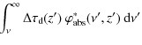
with the abbreviations
confirming the result seen in Fig. 14 to lowest order.
The remaining difference is due mainly to the second order term in Eq. (32)
![]() ,
which we neglected in Eq. (33). The factor
,
which we neglected in Eq. (33). The factor
![]() plays a minor role, since the function
plays a minor role, since the function
![]() varies far more rapidly. We confirmed these statements numerically,
finding that for the considered case the modulation of the blue wing
correction due to
varies far more rapidly. We confirmed these statements numerically,
finding that for the considered case the modulation of the blue wing
correction due to
![]() in the outer integral can be neglected.
in the outer integral can be neglected.
5.2.5 Corrections in the case of

To understand the result when also including the change to the effective emission coefficient
![]() ,
we again look at the red and blue wing contribution separately. Since in the red wing
,
we again look at the red and blue wing contribution separately. Since in the red wing
![]() and because we already saw in Sect. 4.2 that the solution for the spectral distortion is dominated by the correction due to
and because we already saw in Sect. 4.2 that the solution for the spectral distortion is dominated by the correction due to
![]() only (cf. Figs. 5 and 6 right column), we expect that the partial contribution from the red wing will be very close to
only (cf. Figs. 5 and 6 right column), we expect that the partial contribution from the red wing will be very close to
![\begin{displaymath}%
\Delta P^\phi_{\rm rw} \approx \int \phi^\ast_{\rm abs}~[1-F^{\rm t}_\nu]{~\rm d}\nu,
\end{displaymath}](/articles/aa/full_html/2010/04/aa12263-09/img497.png)
where
For the blue wing, one can argue in a very similar way as above. We know that for
![]() the correction to the escape probability is basically given by the time-dependent correction to the value of
the correction to the escape probability is basically given by the time-dependent correction to the value of
![]() ,
but only to higher order because
,
but only to higher order because
![]() .
If now including
.
If now including
![]() ,
the lowest order correction will still be given by the purely
time-dependent case. The additional modulation of the resulting
spectral distortion by
,
the lowest order correction will still be given by the purely
time-dependent case. The additional modulation of the resulting
spectral distortion by
![]() will in addition lead to a small decrease in the total amplitude of the
contribution to the correction. This can again be seen in Fig. 14
when comparing the stars with the short-dashed curve. Only at low
redshifts does the shape of the profile determine the amplitude of the
correction, removing the self-feedback problem. This is because unlike
in the case of
will in addition lead to a small decrease in the total amplitude of the
contribution to the correction. This can again be seen in Fig. 14
when comparing the stars with the short-dashed curve. Only at low
redshifts does the shape of the profile determine the amplitude of the
correction, removing the self-feedback problem. This is because unlike
in the case of
![]() ,
photons are only emitted in a limited range of frequencies. This avoids photons released at
,
photons are only emitted in a limited range of frequencies. This avoids photons released at
![]() and
and
![]() being redshifted into the Lyman
being redshifted into the Lyman ![]() line at
line at ![]() ,
as seen in the normal ``1+1'' formulation of the problem (Chluba & Sunyaev 2009c).
,
as seen in the normal ``1+1'' formulation of the problem (Chluba & Sunyaev 2009c).
Furthermore, it is clear that the sum of both the red and blue wing contribution should again be close to the purely time-dependent case, since the modulation of the contributions from the red (enhancement) and blue wing (suppression) in lowest order will cancel, due to the symmetry around the line center.
![\begin{figure}
\par\includegraphics[width=8.5cm,clip]{eps/12263f33.eps}
\end{figure}](/articles/aa/full_html/2010/04/aa12263-09/img502.png)
|
Figure 15: Relative difference in the effective escape probability with respect to the Sobolev escape probability: combined effect of the thermodynamic correction factor and the shape of the line profile. |
| Open with DEXTER | |
5.3 Combined effect of f and
and

With the derivations in the previous sections, it is now
straightforward to understand the results for the combined effect of
all corrections. Following the same line of thoughts we obtain
![\begin{displaymath}%
\Delta P^{\rm a}_{\rm d}
=-\int\phi^\ast_{\rm abs}~[f_\nu F^{\rm a}_\nu-F^{\phi,\rm qs}_\nu]{~\rm d}\nu.
\end{displaymath}](/articles/aa/full_html/2010/04/aa12263-09/img503.png)
where in
As in the previous section, it is now clear that on the red side of
the resonance the profile will enter the computation mainly because of
its presence in the outer integral. For
![]() and
and
![]() ,
it only leads to a very small correction (cf. Figs. 5 and 6
right column). However, on the blue side of the resonance the profile
correction can again be neglected in the outer integral, but should be
taken into account when computing the difference
,
it only leads to a very small correction (cf. Figs. 5 and 6
right column). However, on the blue side of the resonance the profile
correction can again be neglected in the outer integral, but should be
taken into account when computing the difference
![]() .
One can also conclude that the shape of the profile plays a key role in
removing the low redshift self-feedback problem. The latter statement
can be confirmed when looking at the shape of the Lyman
.
One can also conclude that the shape of the profile plays a key role in
removing the low redshift self-feedback problem. The latter statement
can be confirmed when looking at the shape of the Lyman ![]() distortion at intermediate to high frequencies blueward of the resonance (cf. Figs. 5 and 6 right column), which is clearly dominated by the profile rather than
distortion at intermediate to high frequencies blueward of the resonance (cf. Figs. 5 and 6 right column), which is clearly dominated by the profile rather than ![]() .
.
Therefore, to lowest order one expects the total correction to be the
superposition of the time-dependent correction and the one from the
thermodynamic correction factor, where on the red side of the resonance
each of them is also modulated by the profile shape in the outer
integral of Eq. (35), while on the blue side the contribution is slightly suppressed because of the profile corrections to
![]() .
Here it is important that because
.
Here it is important that because ![]() strongly changes the symmetry of the problem (the main correction originates in the red wing as shown in Sect. 5.1), it is clear that the main effect of
strongly changes the symmetry of the problem (the main correction originates in the red wing as shown in Sect. 5.1), it is clear that the main effect of
![]() will be an enhancement of the final correction.
will be an enhancement of the final correction.
In Fig. 15, we present the results from our numerical calculation for different cases. We find that when including the shape of the profile the corresponding correction is slightly increased as explained above.
![\begin{figure}
\par\includegraphics[width=8.5cm,clip]{eps/12263f34.eps}
\end{figure}](/articles/aa/full_html/2010/04/aa12263-09/img507.png)
|
Figure 16: Total relative difference in the effective escape probability with respect to the Sobolev escape probability: dependence on the total number of shells. Note that the curves for the 5-shell and 10-shell cases practically coincide. |
| Open with DEXTER | |
5.3.1 Dependence on the included number of shells
For the purely time-dependent correction, it has been shown that at low
redshifts in particular the result depends strongly on the total number
of shells that are included in the computation. Since the correction is
strongly dominated by the self-feedback of Lyman ![]() photons, we do expect this dependence on the number of shells to be more mild.
photons, we do expect this dependence on the number of shells to be more mild.
In Fig. 16,
we show the results of our computations for 3, 5, and
10 shells. The changes between the 3 and 5-shell cases is
still rather significant, but the difference between the 5 and
10-shell case is already very minor. This shows that in our
description the total correction has already converged when including ![]() shells into the computation.
shells into the computation.
6 Effect on the ionization history and the CMB power spectra
We now determine the expected correction to the ionization history when including the processes discussed in this paper. For this, we modified the R ECFAST code (Seager et al. 1999), so that we can load the precomputed change to the Sobolev escape probability studied here.
In Fig. 17, we present the final curves for
![]() as obtained for the different processes discussed in this paper. In Fig. 18, we show the corresponding correction to the free electron fraction computed with the modified version of R ECFAST.
One can clearly see that the dominant correction is due to the thermodynamic factor, resulting in
as obtained for the different processes discussed in this paper. In Fig. 18, we show the corresponding correction to the free electron fraction computed with the modified version of R ECFAST.
One can clearly see that the dominant correction is due to the thermodynamic factor, resulting in
![]() at
at
![]() and
and
![]() at
at
![]() .
The next largest correction is related to the time-dependent aspects of the problem, leading to
.
The next largest correction is related to the time-dependent aspects of the problem, leading to
![]() at
at
![]() and
and
![]() at
at
![]() .
The associated correction to the free electron fraction has a maximum of
.
The associated correction to the free electron fraction has a maximum of
![]() at
at
![]() .
The smallest correction is due to the exact shape of the effective line profile, resulting in
.
The smallest correction is due to the exact shape of the effective line profile, resulting in
![]() at
at
![]() and
and
![]() at
at
![]() .
The total correction then is
.
The total correction then is
![]() at
at
![]() and
and
![]() at
at
![]() .
This represents an important acceleration of hydrogen recombination, although at
.
This represents an important acceleration of hydrogen recombination, although at
![]() ,
a large part of the correction due to
,
a large part of the correction due to ![]() alone is canceled by the time-dependent correction. At the maximum of the Thomson visibility function at
alone is canceled by the time-dependent correction. At the maximum of the Thomson visibility function at
![]() ,
we find that
,
we find that
![]() ,
where about
,
where about
![]() is coming from the shape of the profile alone.
is coming from the shape of the profile alone.
![\begin{figure}
\par\includegraphics[width=8.5cm,clip]{eps/12263f35.eps}
\end{figure}](/articles/aa/full_html/2010/04/aa12263-09/img521.png)
|
Figure 17: Relative difference in the effective escape probability with respect to the Sobolev escape probability: separate contributions due to the time-dependent correction, the thermodynamic factor and the shape of the profile. |
| Open with DEXTER | |
![\begin{figure}
\par\includegraphics[width=8.5cm,clip]{eps/12263f36.eps}
\end{figure}](/articles/aa/full_html/2010/04/aa12263-09/img522.png)
|
Figure 18: Changes in the free electron fraction: separate contributions due to the time-dependent correction, the thermodynamic factor and the shape of the profile. |
| Open with DEXTER | |
For completeness, we also show the correction due to the two-photon
formulation alone, i.e., after subtracting the time-dependent
contribution from the total correction. It leads to
![]() at
at
![]() .
.
![\begin{figure}
\par\includegraphics[width=8.5cm,clip]{eps/12263f37.eps}
\end{figure}](/articles/aa/full_html/2010/04/aa12263-09/img523.png)
|
Figure 19: Changes in the CMB temperature and polarization power spectra. We included effect of the time-dependent correction, the thermodynamic correction factor and the profile correction, simultaneously. We used the result for the 10-shell hydrogen atom. |
| Open with DEXTER | |
In Fig. 19, we finally show the changes in the CMB temperature and polarization power spectra coming from the total correction
![]() as given by the solid line in Fig. 18. In particular the changes in the EE power spectrum are impressive, with a peak-to-peak amplitude of
as given by the solid line in Fig. 18. In particular the changes in the EE power spectrum are impressive, with a peak-to-peak amplitude of
![]() at
at ![]() .
One can also see that the modifications to the Cl's
correspond more to a shift in the positions of the peaks rather than
changes in the absolute amplitude. This is because the correction in
the free electron fraction leads to a small shift in the maximum of the
Thomson visibility, but does not affect the Silk damping length (Silk 1968) as much. It will be very important to take these changes into account in the analysis of future CMB data.
.
One can also see that the modifications to the Cl's
correspond more to a shift in the positions of the peaks rather than
changes in the absolute amplitude. This is because the correction in
the free electron fraction leads to a small shift in the maximum of the
Thomson visibility, but does not affect the Silk damping length (Silk 1968) as much. It will be very important to take these changes into account in the analysis of future CMB data.
7 Discussion and conclusions
We have presented a formulation of the Lyman ![]() transfer equation, which allows us to include the two-photon
corrections for the 3s-1s and 3d-1s channels. We then solved this
transfer equation and presented the results for the Lyman
transfer equation, which allows us to include the two-photon
corrections for the 3s-1s and 3d-1s channels. We then solved this
transfer equation and presented the results for the Lyman ![]() distortion at different redshifts (Sect. 4). From this we computed the effective Lyman
distortion at different redshifts (Sect. 4). From this we computed the effective Lyman ![]() escape probability and derived the corresponding corrections to the Sobolev escape probability (Sect. 5).
We used these results to compute the corrections to the free electron
fraction during hydrogen recombination, and the associated changes to
the CMB power spectra (Sect. 6). Below we briefly summarize the results of each section and also provide a short discussion of future work and improvements.
escape probability and derived the corresponding corrections to the Sobolev escape probability (Sect. 5).
We used these results to compute the corrections to the free electron
fraction during hydrogen recombination, and the associated changes to
the CMB power spectra (Sect. 6). Below we briefly summarize the results of each section and also provide a short discussion of future work and improvements.
7.1 The resulting Lyman
spectral distortion
In Sect. 4, we discussed the influence of the different processes on the Lyman ![]() distortion at different redshifts. Including all the corrections considered here simultaneously, one can conclude that at
distortion at different redshifts. Including all the corrections considered here simultaneously, one can conclude that at
![]() the shape of the distortion is determined mainly by the time-dependence of the effective emission rate (cf. Figs. 5 and 6, right column). In the close vicinity of the resonance, all sources of corrections under discussion here are important to the exact shape of the Lyman
the shape of the distortion is determined mainly by the time-dependence of the effective emission rate (cf. Figs. 5 and 6, right column). In the close vicinity of the resonance, all sources of corrections under discussion here are important to the exact shape of the Lyman ![]() spectral distortion at different redshifts (cf. Fig. 4).
In particular, inside the Doppler core the spectral distortion
will be very close to the value at the line center multiplied by
spectral distortion at different redshifts (cf. Fig. 4).
In particular, inside the Doppler core the spectral distortion
will be very close to the value at the line center multiplied by ![]() .
On the blue wing, the distortion is mainly determined by the shape of the line profile.
.
On the blue wing, the distortion is mainly determined by the shape of the line profile.
With the method given here, we can in principle also compute the Lyman ![]() distortion,
as it would be observable today. Since all the processes discussed
here affect the precise shape of this distortion, one could in
principle probe our understanding of the recombination dynamics by
observing it. As mentioned earlier (Chluba & Sunyaev 2009c), one similarly expects additional changes to the detailed shape of the Lyman
distortion,
as it would be observable today. Since all the processes discussed
here affect the precise shape of this distortion, one could in
principle probe our understanding of the recombination dynamics by
observing it. As mentioned earlier (Chluba & Sunyaev 2009c), one similarly expects additional changes to the detailed shape of the Lyman ![]() distortion
because of partial frequency redistribution and electron scattering.
All of these processes therefore not only affect the dynamics of
cosmological hydrogen recombination, but in principle should leave
observable traces in cosmological recombination spectrum (e.g., see Sunyaev & Chluba 2007, and references therein) until today. Measuring the exact shape of the Lyman
distortion
because of partial frequency redistribution and electron scattering.
All of these processes therefore not only affect the dynamics of
cosmological hydrogen recombination, but in principle should leave
observable traces in cosmological recombination spectrum (e.g., see Sunyaev & Chluba 2007, and references therein) until today. Measuring the exact shape of the Lyman ![]() distortion
and the other recombinational lines would in principle allow us to
reveal these differences, and therefore directly probe our
understanding of the recombination problem. Also if something
non-standard happens (e.g., due to early energy release by decaying or
annihilating dark matter), this will affect the exact shape of the
cosmological recombination radiation (Chluba & Sunyaev 2009b).
Therefore, by observing the recombinational radiation one in principle
can directly uncover potential unknowns in the cosmological
recombination problem, a task that may not be otherwise completed.
distortion
and the other recombinational lines would in principle allow us to
reveal these differences, and therefore directly probe our
understanding of the recombination problem. Also if something
non-standard happens (e.g., due to early energy release by decaying or
annihilating dark matter), this will affect the exact shape of the
cosmological recombination radiation (Chluba & Sunyaev 2009b).
Therefore, by observing the recombinational radiation one in principle
can directly uncover potential unknowns in the cosmological
recombination problem, a task that may not be otherwise completed.
7.2 Corrections to the escape probability
We have discussed the corrections to the effective Lyman ![]() escape probability, showing that the largest contribution is from the thermodynamic factor
escape probability, showing that the largest contribution is from the thermodynamic factor ![]() (see Fig. 17).
The next largest correction is related to time-dependent aspects of the
recombination problem, where in the formulation given here the
self-feedback problem (Chluba & Sunyaev 2009c) appearing at low redshifts, disappears when using the ``1+1'' photon picture (cf. Fig. 17).
Furthermore the time-dependent correction partially cancels the correction to the thermodynamic factor at low redshift (
(see Fig. 17).
The next largest correction is related to time-dependent aspects of the
recombination problem, where in the formulation given here the
self-feedback problem (Chluba & Sunyaev 2009c) appearing at low redshifts, disappears when using the ``1+1'' photon picture (cf. Fig. 17).
Furthermore the time-dependent correction partially cancels the correction to the thermodynamic factor at low redshift (
![]() ), leaving a significantly smaller change in the escape probability at
), leaving a significantly smaller change in the escape probability at
![]() .
As we explained here, these two corrections can also be obtained
in the normal ``1+1'' photon picture, but for the thermodynamic
correction factor a natural interpretation can only be given within the
two-photon picture (see Sect. 2.1.1).
Here the crucial ingredient is that the spectrum in the vicinity of the second, low frequency photon
.
As we explained here, these two corrections can also be obtained
in the normal ``1+1'' photon picture, but for the thermodynamic
correction factor a natural interpretation can only be given within the
two-photon picture (see Sect. 2.1.1).
Here the crucial ingredient is that the spectrum in the vicinity of the second, low frequency photon ![]() is given by the CMB blackbody photon field, which then allows us
to write the radiative transfer equation for the Lyman
is given by the CMB blackbody photon field, which then allows us
to write the radiative transfer equation for the Lyman ![]() photon
as an equation for one photon only.
A very similar formulation should be applicable to expanding
envelopes of planetary nebulae and stars, where the photon field in the
vicinity of
photon
as an equation for one photon only.
A very similar formulation should be applicable to expanding
envelopes of planetary nebulae and stars, where the photon field in the
vicinity of ![]() will be given by a weakly diluted blackbody spectrum. However, when the photon distribution in the vicinity of both photons involved in the absorption process are far from their equilibrium values the derived formulation does not work.
will be given by a weakly diluted blackbody spectrum. However, when the photon distribution in the vicinity of both photons involved in the absorption process are far from their equilibrium values the derived formulation does not work.
We also showed that the correction coming from the exact shape of the line profile in the vicinity of the Lyman ![]() resonance
leads to the smallest separate correction under discussion here.
Only this part of the correction is really related to quantum
mechanical modifications of the transfer problem. However, the final
contribution related to this modification is significant at the
required level of accuracy (cf. Fig. 17).
resonance
leads to the smallest separate correction under discussion here.
Only this part of the correction is really related to quantum
mechanical modifications of the transfer problem. However, the final
contribution related to this modification is significant at the
required level of accuracy (cf. Fig. 17).
7.3 Implications for the ionization history and the CMB power spectra and critical remarks
The results for the changes in the free electron fraction and CMB power spectra are shown in Figs. 18 and 19, respectively. The main effect on ![]() due to the processes discussed here is a net acceleration of hydrogen recombination by
due to the processes discussed here is a net acceleration of hydrogen recombination by
![]() at
at
![]() .
About
.
About
![]() of this correction is from the shape of the line profile alone, while
the rest is due to the thermodynamic factor and the time-dependent
aspects of the recombination problem. Here we emphasize again, that the
latter two corrections can also be obtained in the standard
``1+1'' photon picture, when introducing the thermodynamic
correction factor using the detailed balance principle.
of this correction is from the shape of the line profile alone, while
the rest is due to the thermodynamic factor and the time-dependent
aspects of the recombination problem. Here we emphasize again, that the
latter two corrections can also be obtained in the standard
``1+1'' photon picture, when introducing the thermodynamic
correction factor using the detailed balance principle.
We also mention that our results for the changes in the free electron fraction seem to be rather similar to those of Hirata (2008) for the contributions from high level two-photon decays alone. However, we have obtained these results with a completely independent method. For the future, it will be very important to perform a more detailed comparison once all relevant additions are identified.
Regarding the CMB power spectra, in particular the associated changes
in the EE power spectrum are impressive, reaching peak-to-peak
amplitude
![]() at
at ![]() (see Fig. 19).
It will be important to take these corrections into account for the analysis of future CMB data.
(see Fig. 19).
It will be important to take these corrections into account for the analysis of future CMB data.
However, it is also clear that several steps still have to be taken: one still has to (i) study more processes; and (ii) develop a sufficiently fast method to simultaneously incorporate all the corrections discussed in the literature into the computations of the CMB power spectra, in preparation for true parameter estimations using the CMB data.
Regarding the first point, for example, the correction related to Raman processes (as explained in Hirata 2008, mostly due to 2s-1s Raman scattering) leads to an additional delay of recombination at low redshifts with a maximum of
![]() at
at ![]() .
We did not include this process here, but it certainly is very
important to accurate predictions of the CMB power spectra and
should be cross-validated in the future. It is clear that one
should also include the effect of higher level two-photon decays
(e.g., from the 4d-level), since they are expected to also speed
up hydrogen recombination, likely affecting the result obtained here by
another
.
We did not include this process here, but it certainly is very
important to accurate predictions of the CMB power spectra and
should be cross-validated in the future. It is clear that one
should also include the effect of higher level two-photon decays
(e.g., from the 4d-level), since they are expected to also speed
up hydrogen recombination, likely affecting the result obtained here by
another
![]() (i.e.,
(i.e.,
![]() ).
Finally, the effects of partial frequency redistribution, line recoil,
and electron scattering should also be studied. In particular, the
effect of line recoil will be important, leading to a systematic drift
of photons towards lower frequencies again accelerating hydrogen
recombination by
).
Finally, the effects of partial frequency redistribution, line recoil,
and electron scattering should also be studied. In particular, the
effect of line recoil will be important, leading to a systematic drift
of photons towards lower frequencies again accelerating hydrogen
recombination by
![]() at
at ![]() (Chluba & Sunyaev 2009a; Grachev & Dubrovich 2008).
(Chluba & Sunyaev 2009a; Grachev & Dubrovich 2008).
Regarding the second point, Fendt et al. (2009) proposed a new approach called R ICO![]() ,
which uses multi-dimensional polynomial regression to accurately
represent the dependence of the free electron fraction on redshift and
the cosmological parameters. Instead of running the full (slow)
recombination code, one trains R ICO with a set of
models, so that the interpolation between them will be afterwards very
fast.
This approach should allow us to propagate all the corrections in the
ionization history that are included in the full recombination code to
the CMB power spectra, without using any fudging like in R ECFAST (Wong et al. 2008; Seager et al. 1999). In the future, we plan to provide an updated training set for R ICO,
including the corrections discussed here. This should also make
it easier for other groups to cross-validate our results and will allow
us to focus our efforts on the physics rather than our
approximations of it.
,
which uses multi-dimensional polynomial regression to accurately
represent the dependence of the free electron fraction on redshift and
the cosmological parameters. Instead of running the full (slow)
recombination code, one trains R ICO with a set of
models, so that the interpolation between them will be afterwards very
fast.
This approach should allow us to propagate all the corrections in the
ionization history that are included in the full recombination code to
the CMB power spectra, without using any fudging like in R ECFAST (Wong et al. 2008; Seager et al. 1999). In the future, we plan to provide an updated training set for R ICO,
including the corrections discussed here. This should also make
it easier for other groups to cross-validate our results and will allow
us to focus our efforts on the physics rather than our
approximations of it.
Appendix A: Different channels for the emission and death of Lyman
photon involving a sequence of two transitions
If we restrict ourselves to the main channels that can lead to the
emission or absorption of photons in the vicinity of the Lyman ![]() resonance and involve two photons then we are left with: (i)
resonance and involve two photons then we are left with: (i)
![]() two-photon decay and absorption; (ii)
two-photon decay and absorption; (ii)
![]() two-photon decay and absorption; (iii)
two-photon decay and absorption; (iii)
![]() two-photon
recombination and photoionization.
two-photon
recombination and photoionization.
The problem is now to compute the emission and absorption profiles
connected with these processes and describe their relative
contributions or probabilities at a given frequency. This in principle
can be done for all possible routes. However, here we focus on
formulating the problem for the
![]() and
and
![]() two-photon channels, not altering all other channels. This is a
reasonable first approximation, since as we show here it is already
clear from the ``1+1'' photon picture that the main contribution
to the death of
photons is from the 3d channel (see Fig. 1). We only also add the 3s channel, since it is conceptually very similar.
two-photon channels, not altering all other channels. This is a
reasonable first approximation, since as we show here it is already
clear from the ``1+1'' photon picture that the main contribution
to the death of
photons is from the 3d channel (see Fig. 1). We only also add the 3s channel, since it is conceptually very similar.
A.1 The 3s-1s two-photon channel
We derive the rate equation that describes the evolution of the population,
![]() ,
in the 3s level, but where we take into account the two-photon
aspect of the 3s-1s transition. In the normal ``1+1'' photon
picture, this transition is described by the sequence
,
in the 3s level, but where we take into account the two-photon
aspect of the 3s-1s transition. In the normal ``1+1'' photon
picture, this transition is described by the sequence
![]() and its inverse process
and its inverse process
![]() .
For the 3s rate equation, it is therefore clear that the
two-photon correction due to the 3s-1s channel should affect part
of the
.
For the 3s rate equation, it is therefore clear that the
two-photon correction due to the 3s-1s channel should affect part
of the
![]() and
and
![]() rate. Once this part is known, one can in principle replace it in the
rate equations using a more complete two-photon description.
rate. Once this part is known, one can in principle replace it in the
rate equations using a more complete two-photon description.
Here we provide the formulation of this problem, also because
it allows to understand the most important aspects of the two-photon
picture. However, to compute the corrections to the escape probability
we directly use the (precomputed) solution for the populations given in
the standard approach, and only solve for the presumably small
correction to the evolution of the photon field around the Lyman ![]() resonance.
Solving the complete set of modified rate equations simultaneously will
be the final goal, for which one will need the results of the
derivation presented here. We leave this problem to future work.
resonance.
Solving the complete set of modified rate equations simultaneously will
be the final goal, for which one will need the results of the
derivation presented here. We leave this problem to future work.
A.1.1 Isolating the different ``1 + 1'' photon routes
To isolate the contribution from the 3s-1s two-photon channel, we
start by writing down the 3s rate equation in the ``1+1'' photon
picture, including all possible ways for electrons in and out of the
3s-level
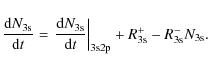
Here we directly separated the part due to the Balmer
which we discuss below in more detail. Here Ni and gi denote the population and statistical weight of level i,
where
Now we are interested in refining the term connected with the Balmer ![]() channel.
Since any two-photon or multi-photon process only leads to tiny
corrections in the total decay rates, it is possible to use the
one-photon rates to compute the relative contributions of different
transition sequences. It is clear that the term
channel.
Since any two-photon or multi-photon process only leads to tiny
corrections in the total decay rates, it is possible to use the
one-photon rates to compute the relative contributions of different
transition sequences. It is clear that the term
![]() describes the total flow of electrons in the direction of the 2p-state.
Once the electron has reached there, it can return to the 3s level
with the probability
describes the total flow of electrons in the direction of the 2p-state.
Once the electron has reached there, it can return to the 3s level
with the probability

Here

Similarly, the electron can take the route

or any of the other channels (
It is then clear that the term
![]() can be interpreted as
can be interpreted as
![\begin{displaymath}%
N_{\rm 3s}~A^{\ast}_{\rm 3s2p} \equiv N_{\rm 3s}~A^{\ast}_{\rm 3s2p}
\times[p_{\rm 2p1s}+\bar{p}_{\rm 2p1s}],
\end{displaymath}](/articles/aa/full_html/2010/04/aa12263-09/img568.png)
because the total flow of electrons should divided into those electrons that go to the 1s-level (probability
From the physical point of view, it is now clear that the partial flow connected with
![]() should be interpreted as 3s-1s two-photon emission in
the ``1+1''-photon picture, which we later replace with the more proper two-photon formulae.
The rest (
should be interpreted as 3s-1s two-photon emission in
the ``1+1''-photon picture, which we later replace with the more proper two-photon formulae.
The rest (
![]() )
describes the contributions of all the other possible channels, e.g., also including the Balmer
)
describes the contributions of all the other possible channels, e.g., also including the Balmer ![]() scattering transition
scattering transition
![]() .
We continue to describe all these in the ``1+1'' photon picture.
.
We continue to describe all these in the ``1+1'' photon picture.
To understand the term connected to the total flow of electrons from the 2p-level towards the 3s-state, given by
![]() ,
we must consider an electron that is added to the 2p-state. It will take the route
,
we must consider an electron that is added to the 2p-state. It will take the route
![]() with probability
with probability
![]() as given by Eq. (A.5). If we consider all
possible routes into the 2p-state, and write the corresponding total rate as
as given by Eq. (A.5). If we consider all
possible routes into the 2p-state, and write the corresponding total rate as
![]() ,
then one has the identity
,
then one has the identity
![\begin{displaymath}%
N_{\rm 2p}~A_{\rm 3s2p}~\frac{g_{\rm 3s}}{g_{\rm 2p}} ~{n_{...
...rm 1s}\frac{g_{\rm 2p}}{g_{\rm
1s}}~A_{\rm 2p1s}~n(\nu_{21})]
\end{displaymath}](/articles/aa/full_html/2010/04/aa12263-09/img578.png)
where
![\begin{displaymath}%
R^{+}_{\rm 2p} =N_{\rm e}N_{\rm p} R_{\rm c 2p}+\sum_{i>2\rm p} N_i~A_{\it i \rm 2p}~[1+{n_{\rm pl}}(\nu_{\it i \rm 2p })].
\end{displaymath}](/articles/aa/full_html/2010/04/aa12263-09/img579.png)
One can now write
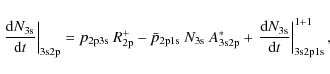
where

The first two terms in Eq. (A.10a) describe the partial flow of electrons towards the 3s-state, but only where it is certain that the electron did not pass through the Lyman
If we now identify

then we can finally rewrite Eq. (A.10b) as

We note that in a vacuum, one would have
A.1.2 Replacing the 3s-1s channel in the ``1 + 1'' photon formulation with the two-photon expression
We now wish to replace the part due to
![]() with
the more proper two-photon terms. For this we have to consider the
detailed form of the 3s-1s two-photon term. If one considers an
electron that is initially in the 3s-state, then one can use the vacuum
3s-1s two-photon decay profile to derive the emission profile needed to
describe the injection of Lyman
with
the more proper two-photon terms. For this we have to consider the
detailed form of the 3s-1s two-photon term. If one considers an
electron that is initially in the 3s-state, then one can use the vacuum
3s-1s two-photon decay profile to derive the emission profile needed to
describe the injection of Lyman ![]() photons
in the escape problem. Simple formulae for the necessary vacuum
two-photon decay profiles can be found in the literature (Chluba & Sunyaev 2008). We shall normalize these profiles like
photons
in the escape problem. Simple formulae for the necessary vacuum
two-photon decay profiles can be found in the literature (Chluba & Sunyaev 2008). We shall normalize these profiles like
![]() ,
where
,
where
![]() already includes the motion of the
atoms in the same way as for the normal Lorentzian lines, usually leading to the Voigt profiles
(e.g., see Mihalas 1978). For convenience, we chose the Lyman
already includes the motion of the
atoms in the same way as for the normal Lorentzian lines, usually leading to the Voigt profiles
(e.g., see Mihalas 1978). For convenience, we chose the Lyman ![]() Doppler-width,
Doppler-width,
![]() ,
in the normalization.
,
in the normalization.
With this, the net change in the number density of electrons in the
3s level by means of the 3s-1s two-photon channel is given by

where
For the approximation Eq. (A.13b),
three comments should be made: first we have assumed that the main
contributions to the integrals over the two-photon line profiles come
from the
poles close to
![]() and
and
![]() .
Second, we have assumed that the CMB spectral distortion around the Balmer
.
Second, we have assumed that the CMB spectral distortion around the Balmer ![]() line are tiny. The stimulated term in the vicinity of the Lyman
line are tiny. The stimulated term in the vicinity of the Lyman ![]() resonance also is completely negligible, so that we can use
resonance also is completely negligible, so that we can use
![]() instead, without changing anything. And finally, we assumed that only
for the 1s-3s two-photon absorption rate do the deviations of the
CMB spectrum from a blackbody in the vicinity of the Lyman
instead, without changing anything. And finally, we assumed that only
for the 1s-3s two-photon absorption rate do the deviations of the
CMB spectrum from a blackbody in the vicinity of the Lyman ![]() resonance matter.
resonance matter.
The result presented in Eq. (A.13b) is identical to the term given by the ``1+1'' photon picture, Eq. (A.12).
This is unsurprising, since with the above approximations we have
simply turned from the two-photon to the ``1+1'' photon picture.
In order to include the effect of two-photon transitions in to the rate
equation of the 3s-level, we should therefore replace
![]() with the full
integral given by Eq. (A.13a).
with the full
integral given by Eq. (A.13a).
A.1.3 Term in the Lyman
radiative transfer equation
To use the integral (A.13a)
in the computations of the ionization history, we also have to consider
the solution to the CMB spectral distortion in the vicinity of the
Lyman ![]() resonance. We therefore have to explicitly write the 3s-1s two-photon
emission and absorption terms for the evolution of the photon field and
solve the corresponding transfer equation. In particular, we wish
to bring the transfer equation into the form Eq. (4).
resonance. We therefore have to explicitly write the 3s-1s two-photon
emission and absorption terms for the evolution of the photon field and
solve the corresponding transfer equation. In particular, we wish
to bring the transfer equation into the form Eq. (4).
From Eq. (A.13a), it follows directly that

![$\displaystyle \frac{2A^{2\gamma}_{\rm 3s1s}}{4\pi} N_{\rm 3s} \varphi^{2\gamma}_{\rm 3s}(\nu) [1+n(\nu)] [1+n(\nu_{31}-\nu)]$](/articles/aa/full_html/2010/04/aa12263-09/img607.png)

Here the factor of 2 is because per electron two photons are involved, and the factor of
Neglecting the deviations from the blackbody spectrum in the emission term and comparing with Eq. (4), we can identify that


This result shows that the effective profile of the process as expected is given by the two-photon profile for the 3s-1s channel, including the induced terms relative to the values at the Lyman and Balmer
We note that
![]() is no longer normalized to unity. In a vacuum, one would find that
is no longer normalized to unity. In a vacuum, one would find that
![]() ,
while within the CMB blackbody field
,
while within the CMB blackbody field
![]() .
However the relative correction to the overall normalization of the profile due to stimulated emission is of the order of
.
However the relative correction to the overall normalization of the profile due to stimulated emission is of the order of
![]() (see Sect. 5.2.1). One should also mention that because of the symmetry in the profile around
(see Sect. 5.2.1). One should also mention that because of the symmetry in the profile around
![]() ,
by restricting the range of integration to
,
by restricting the range of integration to
![]() one can avoid counting both the Lyman
one can avoid counting both the Lyman ![]() and Balmer
and Balmer ![]() photons. We use this to simplify the numerical integration (see Sect. 2.3.1).
photons. We use this to simplify the numerical integration (see Sect. 2.3.1).
If we now look at the absorption term in Eq. (A.14), using the definitions in Eq. (A.15) we can directly write

|
= | ||

|
(A.16) |
Here we have already assumed that for our problem the important part is the region
![$\displaystyle \left.\frac{1}{c}~\frac{\partial N_{\nu}}{\partial t}\right\vert^...
...m 2p3s}}{g_{\rm 3s}/g_{\rm 2p}}
{\rm e}^{\frac{h[\nu - \nu_{21}]}{kT_{\gamma}}}$](/articles/aa/full_html/2010/04/aa12263-09/img629.png)

![$\displaystyle \qquad\qquad\quad\;\; \stackrel{\stackrel{\nu\gtrsim\nu_{31}/2}{\...
..._{\rm 2p3s}~
{\rm e}^{\frac{h[\nu-\nu_{21}]}{kT_{\gamma}}}\!n(\nu)N_{\rm 1s}.~~$](/articles/aa/full_html/2010/04/aa12263-09/img631.png)
Note that
With the Einstein relations, it is then easy to show that
![]() ,
so that we directly verify the thermodynamic correction factor
,
so that we directly verify the thermodynamic correction factor![]()
![]() and find that
and find that
![]() .
We therefore have confirmed the completeness of the form of Eq. (4) for the 3s-1s two-photon channel.
.
We therefore have confirmed the completeness of the form of Eq. (4) for the 3s-1s two-photon channel.
A.2 The 3d-1s two-photon channel
After going through the argument for the 3s-1s channel, it is easy to do the same for the 3d-1s channel. For the rate equation analog to Eqs. (A.1), (A.3), and (A.10), one has
| (A.18a) | |||
| (A.18b) | |||
| (A.18c) |
where the Balmer


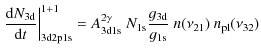
As before, one should now replace Eq. (A.18f) with


if one is interested in the 3d-1s two-photon correction to the 3d-rate equation. We note that here the ratio of the statistical weights is not unity as for the 3s-1s channel.
The terms for the transfer equation can also be cast in the form of Eq. (4) where the important coefficients are given by
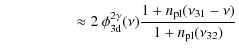
A.3 The other channels
For the other channels in and out of the 2p-state, we can also
derive the corresponding partial rates in a similar way as for the 3s
and 3d state. However, since the main correction is expected to
come from the 3s and 3d two-photon channels for these we simply
use the ``1+1'' photon picture. This means that we will not
replace the corresponding
![]() rates with the two-photon description. For all the ns and nd-states with n>3, the rate equations will therefore be similar to Eq. (A.18), and for electrons in the continuum one will have
rates with the two-photon description. For all the ns and nd-states with n>3, the rate equations will therefore be similar to Eq. (A.18), and for electrons in the continuum one will have
![\begin{displaymath}%
\frac{{\rm d} N_{\rm e}}{{\rm d} t} =\left.\frac{{\rm d} N_...
...i \rm c} N_{i} - N_{\rm e} N_{\rm p} R_{\rm c \it i}
\right],
\end{displaymath}](/articles/aa/full_html/2010/04/aa12263-09/img654.png)
where
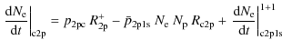


There remains a small difference to the normal rate equations. In the formulation given above, the population of the 2p-state has vanished from all the rate equations, and in particular from those for the 3s and 3d-state. For the 3s and 3d-state, this is physically expected, since in the two-photon picture on the way to the 1s-level the electron does not really pass through the 2p-state. In the full two-photon picture, the electron reaches the 1s level via all intermediate p-states, including those in the continuum. For the other levels, the above formulation would have also been obtained by simply replacing the solution of the 2p-state with the quasi-stationary value in the ``1+1'' photon approach. In this way, one again has a closed system of rate equations, which avoids the difficulty of attaching a population to the 2p-state.
Appendix B: Derivation of the thermodynamic factor using the ``1 + 1'' photon picture
As mentioned in the introduction and also earlier (Chluba & Sunyaev 2009c), in the normal ``1+1'' photon approximation the term describing the emission and absorption of Lyman ![]() photons in full thermodynamic equilibrium does not exactly conserve a blackbody spectrum at all frequencies. This can be directly seen from Eq. (1), since in full thermodynamic equilibrium one should have
photons in full thermodynamic equilibrium does not exactly conserve a blackbody spectrum at all frequencies. This can be directly seen from Eq. (1), since in full thermodynamic equilibrium one should have
![]() .
Using the definitions of the previous section, in equilibrium one expects
.
Using the definitions of the previous section, in equilibrium one expects
![]() ,
,
![]() ,
,
![]() ,
and
,
and
![]() ,
so that one finds
,
so that one finds
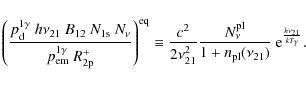
Here
![\begin{displaymath}%
\left(
\frac{p^{\rm 1\gamma}_{\rm d}~h\nu_{\rm 21}~B_{12}~...
...\rm e}^{\frac{h[\nu_{21}-\nu]}{kT_{\gamma}}}
\approx 1/f_{\nu}
\end{displaymath}](/articles/aa/full_html/2010/04/aa12263-09/img666.png)
In the last step, we assumed that
![\begin{displaymath}%
p^{1\gamma, \ast}_{\rm em} =\frac{A_{\rm 2p1s}}{A_{\rm 2p1s}[1+\left<n_{\nu}\right>_{\rm em}]+R^{-}_{\rm 2p}}\cdot
\end{displaymath}](/articles/aa/full_html/2010/04/aa12263-09/img669.png)
Here
We mention another way to obtain the thermodynamic factor in the absorption process, which just uses the term in the Lyman ![]() rate equation. In the standard textbooks (e.g., Mihalas 1978), one finds that
rate equation. In the standard textbooks (e.g., Mihalas 1978), one finds that
![\begin{displaymath}%
\left.\frac{{\rm d} N_{\rm 2p}}{{\rm d} t}\right\vert _{\rm...
...\rm 2p1s}~n(\nu_{21})
-N_{\rm 2p}~A_{\rm 2p1s}[1+n(\nu_{21})].
\end{displaymath}](/articles/aa/full_html/2010/04/aa12263-09/img671.png)
Here two comments should be made: (i) more rigorously one should replace

It is now easy to show that
![$\displaystyle \left<\frac{n^{\rm pl}_{\nu}}{1+n^{\rm pl}_{\nu}}~[1+n^{\rm pl}_{\nu}]\right>_{\rm abs}~{\rm e}^{h\nu_{21}/kT_{\gamma}}$](/articles/aa/full_html/2010/04/aa12263-09/img679.png)
Since according to Eq. (B.5)
Appendix C: Computation of two-photon profiles
We compute the two-photon decay profiles according to the work of Chluba & Sunyaev (2009c).
There in particular the infinite sum over intermediate states was
divided into two sets of states with principal quantum numbers n>ni and ![]() ,
where ni is
the initial state principal quantum number. This makes the sum over the
resonances (in the case of 3s and 3d, only one)
finite and allows us to give fitting formulae for the remaining
contribution to the total matrix element from the infinite sum. This
procedure is very convenient for numerical evaluations.
,
where ni is
the initial state principal quantum number. This makes the sum over the
resonances (in the case of 3s and 3d, only one)
finite and allows us to give fitting formulae for the remaining
contribution to the total matrix element from the infinite sum. This
procedure is very convenient for numerical evaluations.
Here we would like to mention that the two-photon decay profiles behave like
![]() in the limits
in the limits
![]() or
or
![]() .
This is because in this limit the main term in the infinite sum originates in the matrix element
.
This is because in this limit the main term in the infinite sum originates in the matrix element
![]() ,
which in the non-relativistic formulation has zero transition frequency. This implies that for
,
which in the non-relativistic formulation has zero transition frequency. This implies that for
![]() or
or
![]()

Here 1|4 means 1 for the s-states or 4 for the d-states. Inserting numbers (for definitions see Chluba & Sunyaev 2008), one finds

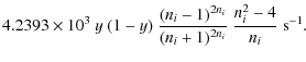
For the 3s and 3d profiles, one therefore has
We use these simple formulae to compute the two-photon spectra at
The most important consequence of this limiting behavior with
frequency is that because of stimulated emission in the ambient
CMB blackbody radiation field the two-photon profiles no longer
vanish at ![]() and
and ![]() ,
since
,
since
![]() for
for ![]() .
For the 2s-1s two-photon process, this behavior was also seen earlier (Chluba & Sunyaev 2006b). In the case of 3s and 3d two-photon decays, this enhances the emission of photons close to the Lyman
.
For the 2s-1s two-photon process, this behavior was also seen earlier (Chluba & Sunyaev 2006b). In the case of 3s and 3d two-photon decays, this enhances the emission of photons close to the Lyman ![]() resonance (cf. Fig. 2).
However, we find that the corrections due to stimulated two-photon
emission are not important for the cosmological recombination problem.
resonance (cf. Fig. 2).
However, we find that the corrections due to stimulated two-photon
emission are not important for the cosmological recombination problem.
Appendix D: Small corrections due to the motion of the atom
To account for the motion of the atoms in the computations of the
emission profile, one has to compute the following integral (see
Sect. 9.2 in Mihalas 1978)
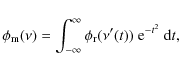
over the rest-frame emission profile,
For the Voigt profile, one normally uses the approximation
![]() ,
so that the emission profile can be written in terms of the Voigt function
,
so that the emission profile can be written in terms of the Voigt function
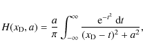
for which simple approximation in terms of the Dawson-integral exist (see Sect. 9.2 in Mihalas 1978). Here a is the normal Voigt parameter, and
![\begin{figure}
\par\includegraphics[width=8.5cm,clip]{eps/12263f38.eps}
\end{figure}](/articles/aa/full_html/2010/04/aa12263-09/img715.png)
|
Figure D.1:
Small correction to the normal Voigt profile. We show the relative difference of the standard Voigt profile
|
| Open with DEXTER | |
However, because of the steepness of the Lorentzian close to the line center this approximation leads to a small inaccuracy (
![]() ), which is not necessary.
To avoid this, one should simply replace
), which is not necessary.
To avoid this, one should simply replace
![]() and a in the Voigt integral with
and a in the Voigt integral with
![]() and
and
![]() ,
and in addition multiply H with
,
and in addition multiply H with
![]() ,
yielding
,
yielding
![\begin{displaymath}%
\tilde{H}({{x_{\rm D}}}, a) =
\frac{H(\tilde{x}_{\rm D}, \t...
...a})}{[1+{{x_{\rm D}}}\frac{\Delta\nu_{\rm D}}{\nu_{21}}]}\cdot
\end{displaymath}](/articles/aa/full_html/2010/04/aa12263-09/img720.png)
As one can see, the Voigt profile,
![$\displaystyle \frac{1}{\sqrt{\pi}}~\frac{{\rm e}^{-\tilde{x}_{\rm D}^2}}{[1+{{x_{\rm D}}}\frac{\Delta\nu_{\rm D}}{\nu_{21}}]}$](/articles/aa/full_html/2010/04/aa12263-09/img723.png)
![$\displaystyle \frac{1}{\sqrt{\pi}}~{\rm e}^{-x_{\rm D}^2}\left[1-{{x_{\rm D}}}\frac{\Delta\nu_{\rm D}}{\nu_{21}}(1+2 x_{\rm D}^2)\right]$](/articles/aa/full_html/2010/04/aa12263-09/img724.png)
close to the line center. At
![\begin{figure}
\par\includegraphics[width=8.5cm,clip]{eps/12263f39.eps}
\end{figure}](/articles/aa/full_html/2010/04/aa12263-09/img729.png)
|
Figure D.2: Relative difference of the 3s and 3d two-photon profiles with respect to the Lorentzian (thin line) and the Voigt profile (thick lines). In the first case the motion of the atoms was neglected, while for the comparison with the Voigt profile it was included. The boxes show the analytic approximation for the correction including the motion. |
| Open with DEXTER | |
D.1 Two-photon profiles for moving atoms
As mentioned above, to include the motion of the atoms in the
computation of the two-photon profiles one can in principle directly
use the expression in Eq. (D.1). However, the computation of this integral is rather time-consuming, and in the very distant wings is also unnecessary![]() . Therefore, we use a different approach in which we utilize that the relative difference,
. Therefore, we use a different approach in which we utilize that the relative difference,
![]() ,
between the rest frame two-photon profile,
,
between the rest frame two-photon profile,
![]() ,
and the normal Lorentzian,
,
and the normal Lorentzian,
![]() ,
varies very slowly with frequency, compared to
,
varies very slowly with frequency, compared to
![]() .
Therefore, to lowest order for moving atoms the two-photon profile will be given by
.
Therefore, to lowest order for moving atoms the two-photon profile will be given by
![]() .
.
However, close to the line center this approximation due to the
steepness of the Lorentzian again becomes inaccurate at the percent
level. The lowest order correction can be computed approximating the
rest-frame two-photon profiles close to the Lyman ![]() line center by
line center by
![\begin{displaymath}%
\phi^{2\gamma}_{{\rm r}, i}(\nu)
\approx \phi_{\Lambda}(\nu)[1+\alpha_i+\beta_i~{{x_{\rm D}}}].
\end{displaymath}](/articles/aa/full_html/2010/04/aa12263-09/img735.png)
Here the coefficients
Table D.1:
Parameters for the 3s and 3d two photon profiles around the line center. These were determined in the range
![]() .
For explanation, see Appendix D.
.
For explanation, see Appendix D.
Using the same method as described in Sect. 9.2 of Mihalas (1978), it can then be shown that for
![]()
![\begin{displaymath}%
\phi^{2\gamma}_{{\rm m}, i}({{x_{\rm D}}}, a)
\!\approx\!
\...
...lde{a})}{\tilde{H}(\tilde{x}_{\rm D}, \tilde{a})}
\right]\cdot
\end{displaymath}](/articles/aa/full_html/2010/04/aa12263-09/img744.png)
Close to the line center, we use this expression for the two-photon profiles. However, far away from the Lyman
However, we find that the correction in connection with the motion of the atom are unimportant to the cosmological recombination problem.
References
- Chluba, J., & Sunyaev, R. A. 2006a, A&A, 458, L29 [NASA ADS] [CrossRef] [EDP Sciences] [Google Scholar]
- Chluba, J., & Sunyaev, R. A. 2006b, A&A, 446, 39 [NASA ADS] [CrossRef] [EDP Sciences] [Google Scholar]
- Chluba, J., & Sunyaev, R. A. 2007, A&A, 475, 109 [NASA ADS] [CrossRef] [EDP Sciences] [Google Scholar]
- Chluba, J., & Sunyaev, R. A. 2008, A&A, 480, 629 [NASA ADS] [CrossRef] [EDP Sciences] [Google Scholar]
- Chluba, J., & Sunyaev, R. A. 2009a, A&A, 503, 345 [NASA ADS] [CrossRef] [EDP Sciences] [Google Scholar]
- Chluba, J., & Sunyaev, R. A. 2009b, A&A, 501, 29 [NASA ADS] [CrossRef] [EDP Sciences] [Google Scholar]
- Chluba, J., & Sunyaev, R. A. 2009c, A&A, 496, 619 [NASA ADS] [CrossRef] [EDP Sciences] [Google Scholar]
- Chluba, J., Rubiño-Martín, J. A., & Sunyaev, R. A. 2007, MNRAS, 374, 1310 [NASA ADS] [CrossRef] [Google Scholar]
- Cresser, J. D., Tang, A. Z., Salamo, G. J., & Chan, F. T. 1986, Phys. Rev. A, 33, 1677 [NASA ADS] [CrossRef] [PubMed] [Google Scholar]
- de Bernardis, F., Bean, R., Galli, S., et al. 2009, Phys. Rev. D, 79, 043503 [NASA ADS] [CrossRef] [Google Scholar]
- Dubrovich, V. K., & Grachev, S. I. 2005, Astron. Lett., 31, 359 [NASA ADS] [CrossRef] [Google Scholar]
- Eisenstein, D. J. 2005, New Astron. Rev., 49, 360 [NASA ADS] [CrossRef] [Google Scholar]
- Eisenstein, D. J., Zehavi, I., Hogg, D. W., et al. 2005, ApJ, 633, 560 [NASA ADS] [CrossRef] [Google Scholar]
- Fendt, W. A., Chluba, J., Rubiño-Martín, J. A., & Wandelt, B. D. 2009, ApJS, 181, 627 [NASA ADS] [CrossRef] [Google Scholar]
- Göppert-Mayer 1931, Annalen der Physik, 9, 273 [NASA ADS] [CrossRef] [Google Scholar]
- Grachev, S. I., & Dubrovich, V. K. 2008, Astron. Lett., 34, 439 [NASA ADS] [CrossRef] [Google Scholar]
- Hirata, C. M. 2008, Phys. Rev. D, 78, 023001 [NASA ADS] [CrossRef] [Google Scholar]
- Hu, W., Scott, D., Sugiyama, N., & White, M. 1995, Phys. Rev. D, 52, 5498 [NASA ADS] [CrossRef] [Google Scholar]
- Hütsi, G. 2006, A&A, 449, 891 [NASA ADS] [CrossRef] [EDP Sciences] [Google Scholar]
- Jentschura, U. D. 2009, Phys. Rev. A, 79, 022510 [NASA ADS] [CrossRef] [Google Scholar]
- Jones, B. J. T., & Wyse, R. F. G. 1985, A&A, 149, 144 [NASA ADS] [Google Scholar]
- Karshenboim, S. G., & Ivanov, V. G. 2008, Astron. Lett., 34, 289 [NASA ADS] [CrossRef] [Google Scholar]
- Kholupenko, E. E., & Ivanchik, A. V. 2006, Astron. Lett., 32, 795 [NASA ADS] [CrossRef] [Google Scholar]
- Labzowsky, L., Solovyev, D., & Plunien, G. 2009, Phys. Rev. A, 80, 062514 [NASA ADS] [CrossRef] [Google Scholar]
- Mihalas, D. 1978, Stellar atmospheres/2nd edn./ (San Francisco: W. H. Freeman and Co.), 650 [Google Scholar]
- Peebles, P. J. E. 1968, ApJ, 153, 1 [NASA ADS] [CrossRef] [Google Scholar]
- Peebles, P. J. E., Seager, S., & Hu, W. 2000, ApJ, 539, L1 [NASA ADS] [CrossRef] [Google Scholar]
- Rubiño-Martín, J. A., Chluba, J., & Sunyaev, R. A. 2006, MNRAS, 371, 1939 [NASA ADS] [CrossRef] [Google Scholar]
- Rubiño-Martín, J. A., Chluba, J., & Sunyaev, R. A. 2008, A&A, 485, 377 [NASA ADS] [CrossRef] [EDP Sciences] [Google Scholar]
- Seager, S., Sasselov, D. D., & Scott, D. 1999, ApJ, 523, L1 [NASA ADS] [CrossRef] [Google Scholar]
- Seager, S., Sasselov, D. D., & Scott, D. 2000, ApJS, 128, 407 [NASA ADS] [CrossRef] [Google Scholar]
- Seljak, U., Sugiyama, N., White, M., & Zaldarriaga, M. 2003, Phys. Rev. D, 68, 083507 [NASA ADS] [CrossRef] [Google Scholar]
- Silk, J. 1968, ApJ, 151, 459 [NASA ADS] [CrossRef] [Google Scholar]
- Sunyaev, R. A., & Chluba, J. 2007, Nuovo Cimento B Serie, 122, 919 [NASA ADS] [Google Scholar]
- Sunyaev, R. A., & Chluba, J. 2008, in Frontiers of Astrophysics: A Celebration of NRAO's 50th Anniversary, ed. A. H. Bridle, J. J. Condon, & G. C. Hunt, ASP Conf. Ser., 395, 35 [Google Scholar]
- Sunyaev, R. A., & Zeldovich, Y. B. 1970, Ap&SS, 7, 3 [NASA ADS] [Google Scholar]
- Switzer, E. R., & Hirata, C. M. 2008, Phys. Rev. D, 77, 083006 [NASA ADS] [CrossRef] [Google Scholar]
- Wong, W. Y., & Scott, D. 2007, MNRAS, 375, 1441 [NASA ADS] [CrossRef] [Google Scholar]
- Wong, W. Y., Moss, A., & Scott, D. 2008, MNRAS, 386, 1023 [NASA ADS] [CrossRef] [Google Scholar]
- Zeldovich, Y. B., Kurt, V. G., & Syunyaev, R. A. 1968, Zhurnal Eksperimental noi i Teoreticheskoi Fiziki, 55, 278 [Google Scholar]
Footnotes
- ... Surveyor
![[*]](/icons/foot_motif.png)
- www.rssd.esa.int/Planck
- ... formula
- This expression was first derived by Göppert-Mayer (1931).
- ... modifications
- As already mentioned in Chluba & Sunyaev (2009c), our current version of the code already contains the corrections due to line diffusion on thermal atoms, atomic recoil, and electron scattering. In good agreement with Grachev & Dubrovich (2008), we found that atomic recoil is most important, but partial frequency redistribution only leads to an additional small modification. In Chluba & Sunyaev (2009a), we present the results of these computations, also taking the 3d-1s and 3s-1d two-photon corrections into account.
- ... solutions
- We used the output of the latest version of our multilevel code (Chluba et al. 2007; Rubiño-Martín et al. 2006).
- ... conservation
- For the 1s-3d two-photon absorption, this will be
 ,
where
,
where  is
the corresponding 1s-3d transition frequency and
is
the corresponding 1s-3d transition frequency and  denotes the frequency of the photon that is absorbed in the vicinity of
the Lyman
resonance.
denotes the frequency of the photon that is absorbed in the vicinity of
the Lyman
resonance.
- ... alone
- Note that this is only part of the total correction which was presented in Hirata (2008).
- ... picture
- For formal consistency, we included the factors
 due
to stimulated emission in the ambient CMB blackbody field
in the definition of
due
to stimulated emission in the ambient CMB blackbody field
in the definition of
 ,
although during recombination
,
although during recombination
 .
.
- ... factor
- We added a short derivation for
 in Appendix B.
- ... function
-
 corresponds
to
corresponds
to
![${{x_{\rm D}}}\approx -1.7 \times 10^{4}\left[\frac{1+z}{1100}\right]^{-1/2}$](/articles/aa/full_html/2010/04/aa12263-09/img145.png) Doppler width, so that the absolute error in the normalization
of
Doppler width, so that the absolute error in the normalization
of
 is
is
 .
.
- ... asymmetry
- More clearly, here one should refer to the mixture of quantum mechanical processes important to the emission and absorption profile.
- ... to
- The upper indices will henceforth indicate the included
correction. ``t'' represents the time-dependent correction,
``f'' the thermodynamic factor, and ``
 '' the profile
correction. When all corrections are included simultaneously, we
use ``a''.
'' the profile
correction. When all corrections are included simultaneously, we
use ``a''.
- ... center
- Since in the red wing
 (cf. Fig. 2),
one expects
(cf. Fig. 2),
one expects
 .
.
- ... to
- There is a tiny difference because
 .
.
- ... ICO
- http://cosmos.astro.uiuc.edu/rico/
- ... is
- Here the approximate sign is due to the fact that the rate
coefficient in the two-photon formulation should contain some small (
 )
quantum mechanical correction to the one photon rate. This will not
lead to any significant correction in the escape probability.
)
quantum mechanical correction to the one photon rate. This will not
lead to any significant correction in the escape probability.
- ... factor
- From Eq. (A.17)
by comparing with Eq. (4),
we can see that for our choice of coefficients and variables we can
more rigorously infer
![$f_\nu=\frac{\nu_{21}^2}{\nu^2}{\rm e}^{\frac{h[\nu-\nu_{21}]}{kT_{\gamma}}} \fr...
...}}(\nu)}\approx \frac{\nu_{21}^2}{\nu^2}~{\rm e}^{h[\nu-\nu_{21}]/kT_{\gamma}} $](/articles/aa/full_html/2010/04/aa12263-09/img634.png) for
for  ,
a condition that is fulfilled during cosmological
recombination in the vicinity (
,
a condition that is fulfilled during cosmological
recombination in the vicinity (
 )
of the Lyman
resonance.
)
of the Lyman
resonance.
- ... unnecessary
- There the motion of the atoms can be neglected since the
two-photon profiles normally vary very slowly with frequency. Although
this is not entirely true for the ns two-photon
profiles close to the frequencies where
 vanishes, one expects a
negligible additional correction due to this
approximation.
vanishes, one expects a
negligible additional correction due to this
approximation.
All Tables
Table D.1:
Parameters for the 3s and 3d two photon profiles around the line center. These were determined in the range
![]() .
For explanation, see Appendix D.
.
For explanation, see Appendix D.
All Figures
|
|
Figure 1:
The death probabilities for different Lyman |
| Open with DEXTER | |
| In the text | |
|
|
Figure 2:
Different line profiles in the vicinity of the Lyman |
| Open with DEXTER | |
| In the text | |
|
|
Figure 3:
Modifications in the absorption optical depth
|
| Open with DEXTER | |
| In the text | |
|
|
Figure 4:
Difference in the Lyman |
| Open with DEXTER | |
| In the text | |
|
|
Figure 5:
Difference in the Lyman |
| Open with DEXTER | |
| In the text | |
|
|
Figure 6:
The Lyman |
| Open with DEXTER | |
| In the text | |
|
|
Figure 7:
Source of the asymmetry between the absorption and emission profiles,
|
| Open with DEXTER | |
| In the text | |
|
|
Figure 8:
The functions
|
| Open with DEXTER | |
| In the text | |
|
|
Figure 9: Relative difference in the effective escape probability with respect to the Sobolev escape probability: effect of the thermodynamic correction factor. |
| Open with DEXTER | |
| In the text | |
|
|
Figure 10:
Difference between the effective escape probability and the Sobolev
escape probability: the effect of the thermodynamic correction factor
in the blue and red wing of the resonance. For the upper panel, we set
|
| Open with DEXTER | |
| In the text | |
|
|
Figure 11:
Relative difference in the effective escape probability with respect to
the Sobolev escape probability: effect of the thermodynamic correction
factor at different distances to the line center. For the upper panel we set
|
| Open with DEXTER | |
| In the text | |
|
|
Figure 12: Deviation of the normalization of the different line-profiles from unity. The effect of stimulated emission in the ambient CMB blackbody radiation field was included. |
| Open with DEXTER | |
| In the text | |
|
|
Figure 13: Relative difference in the effective escape probability with respect to the Sobolev escape probability: effect of the line profile. For the curves labeled with ``CS09'' (Chluba & Sunyaev 2009c) we used the standard Voigt profile, while for the others we included the two-photon corrections for the 3s and 3d channels. |
| Open with DEXTER | |
| In the text | |
|
|
Figure 14:
Relative difference in the effective escape probability with respect to
the Sobolev escape probability: correction due to the shape of the
absorption profile in the blue and red wing of the resonance. For the upper panel we set
|
| Open with DEXTER | |
| In the text | |
|
|
Figure 15: Relative difference in the effective escape probability with respect to the Sobolev escape probability: combined effect of the thermodynamic correction factor and the shape of the line profile. |
| Open with DEXTER | |
| In the text | |
|
|
Figure 16: Total relative difference in the effective escape probability with respect to the Sobolev escape probability: dependence on the total number of shells. Note that the curves for the 5-shell and 10-shell cases practically coincide. |
| Open with DEXTER | |
| In the text | |
|
|
Figure 17: Relative difference in the effective escape probability with respect to the Sobolev escape probability: separate contributions due to the time-dependent correction, the thermodynamic factor and the shape of the profile. |
| Open with DEXTER | |
| In the text | |
|
|
Figure 18: Changes in the free electron fraction: separate contributions due to the time-dependent correction, the thermodynamic factor and the shape of the profile. |
| Open with DEXTER | |
| In the text | |
|
|
Figure 19: Changes in the CMB temperature and polarization power spectra. We included effect of the time-dependent correction, the thermodynamic correction factor and the profile correction, simultaneously. We used the result for the 10-shell hydrogen atom. |
| Open with DEXTER | |
| In the text | |
|
|
Figure D.1:
Small correction to the normal Voigt profile. We show the relative difference of the standard Voigt profile
|
| Open with DEXTER | |
| In the text | |
|
|
Figure D.2: Relative difference of the 3s and 3d two-photon profiles with respect to the Lorentzian (thin line) and the Voigt profile (thick lines). In the first case the motion of the atoms was neglected, while for the comparison with the Voigt profile it was included. The boxes show the analytic approximation for the correction including the motion. |
| Open with DEXTER | |
| In the text | |
Copyright ESO 2010
Current usage metrics show cumulative count of Article Views (full-text article views including HTML views, PDF and ePub downloads, according to the available data) and Abstracts Views on Vision4Press platform.
Data correspond to usage on the plateform after 2015. The current usage metrics is available 48-96 hours after online publication and is updated daily on week days.
Initial download of the metrics may take a while.