| Issue |
A&A
Volume 511, February 2010
|
|
|---|---|---|
| Article Number | A66 | |
| Number of page(s) | 14 | |
| Section | Planets and planetary systems | |
| DOI | https://doi.org/10.1051/0004-6361/200913491 | |
| Published online | 11 March 2010 | |
Clouds in the atmospheres of extrasolar planets
I. Climatic effects of multi-layered clouds for Earth-like planets and implications for habitable zones
D. Kitzmann1 - A. B. C. Patzer1 - P. von Paris2 - M. Godolt1 - B. Stracke2 - S. Gebauer1 - J. L. Grenfell1 - H. Rauer1,2
1 - Zentrum für Astronomie und Astrophysik, Technische Universität
Berlin, Hardenbergstr. 36, 10623 Berlin, Germany
2 - Institut für Planetenforschung, Deutsches Zentrum für Luft- und
Raumfahrt (DLR), Rutherfordstr. 2, 12489 Berlin, Germany
Received 16 October 2009 / Accepted 22 December 2009
Abstract
Aims. The effects of multi-layered clouds in the
atmospheres of Earth-like planets orbiting different types of stars are
studied. The radiative effects of cloud particles are directly
correlated with their wavelength-dependent optical properties.
Therefore the incident stellar spectra may play an important role for
the climatic effect of clouds. We discuss the influence of clouds with
mean properties measured in the Earth's atmosphere on the surface
temperatures and Bond albedos of Earth-like planets orbiting different
types of main sequence dwarf stars. The influence of clouds on the
position of the habitable zone around these central star types is
discussed.
Methods. A parametric cloud model has been developed
based on observations in the Earth's atmosphere. The corresponding
optical properties of the cloud particles are calculated with the Mie
theory accounting for shape effects of ice particles by the equivalent
sphere method. The parametric cloud model is linked with a
one-dimensional radiative-convective climate model to study the effect
of clouds on the surface temperature and the Bond albedo of Earth-like
planets in dependence of the type of central star.
Results. The albedo effect of the low-level clouds
depends only weakly on the incident stellar spectra because the optical
properties remain almost constant in the wavelength range of the
maximum of the incident stellar radiation. The greenhouse effect of the
high-level clouds on the other hand depends on the temperature of the
lower atmosphere, which is itself an indirect consequence of the
different types of central stars. In general the planetary Bond albedo
increases with the cloud cover of either cloud type. An anomaly was
found for the K and M-type stars however, resulting in a decreasing
Bond albedo with increasing cloud cover for certain atmospheric
conditions. Depending on the cloud properties, the position of the
habitable zone can be located either farther from or closer to the
central star. As a rule, low-level water clouds lead to a decrease of
distance because of their albedo effect, while the high-level ice
clouds lead to an increase in distance. The maximum variations are
about ![]() decrease and
decrease and ![]() increase in distance compared to the clear sky case for the same mean
Earth surface conditions in each case.
increase in distance compared to the clear sky case for the same mean
Earth surface conditions in each case.
Key words: planetary systems - atmospheric effects - astrobiology
1 Introduction
Cloud particles can have an important impact on the climate of planetary atmospheres by either scattering the incident stellar radiation back to space (albedo effect) or by trapping the infrared radiation in the atmosphere (greenhouse effect). The answer to the question which of these effects dominates for a given cloud type depends on a variety of cloud parameters, the most important of which are the cloud composition (water, carbon dioxide etc.), the size distribution of the cloud particles, the optical depth of the cloud layer, multi-layered cloud coverage and the cloud altitude.
In the case of the well known Earth atmosphere, where clouds
are a very common phenomenon with a mean global cloud coverage of more
than ![]() ,
low-level water clouds have a net cooling effect on the surface, while
high-level ice clouds exhibit a greenhouse effect, resulting in surface
heating. A comprehensive review about the climatic effects of clouds in
the Earth atmosphere can be found in e.g. Kondratyev
(1999) and references therein. The albedo and the greenhouse
effect are directly correlated with the wavelength-dependent optical
properties of the cloud particles. The incident stellar spectra in
combination with these optical properties of the cloud may therefore
play an important role for the surface temperature.
,
low-level water clouds have a net cooling effect on the surface, while
high-level ice clouds exhibit a greenhouse effect, resulting in surface
heating. A comprehensive review about the climatic effects of clouds in
the Earth atmosphere can be found in e.g. Kondratyev
(1999) and references therein. The albedo and the greenhouse
effect are directly correlated with the wavelength-dependent optical
properties of the cloud particles. The incident stellar spectra in
combination with these optical properties of the cloud may therefore
play an important role for the surface temperature.
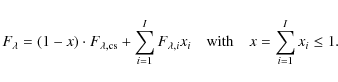
Table 1: Mean cloud properties obtained from surface and satellite measurements.
Model calculations regarding the habitability of planets orbiting different types of central stars have already been done by e.g. Kasting et al. (1993), Segura et al. (2005,2003) or Selsis et al. (2007). Still, these models lack a detailed treatment of the cloud radiative forcing in the radiative transfer and aim only to mimic the cooling effect of low-level clouds by an adjusted surface albedo. Focussing on the inner boundary of the habitable zone around the Sun Kasting (1988) included the effect of one very extended water droplet cloud with rather simplified optical properties in some of the model scenarios. Without taking clouds explicitly into account in their atmospheric climate model calculations Kaltenegger et al. (2007) studied the emission spectra of Earth-like planets at different evolutionary stages.
We study the effects of different incident stellar spectra in conjunction with multi-layered clouds of different types on the surface temperatures of Earth-like extrasolar planets, which determine the potential habitability of a terrestrial planet. As a first approximation, a simplified cloud description scheme using parametrised size distribution functions is used. Other cloud properties like optical depth and cloud top pressure have been taken from measurements. The parametric cloud model is described in Sect. 2. To study the basic climatic effects, our cloud scheme has been coupled with a one-dimensional radiative-convective climate model which includes the possibility to account for different amounts of cloud coverages as well as the partial overlap of two cloud layers, as described in Sect. 3. In Sect. 4 we apply this climate model including the parametrised cloud description to the modern Earth atmosphere to verify the applicability of our model approach. Resulting surface temperatures and Bond albedos for different cloud types in the atmospheres of Earth-like planets orbiting different types of central stars and implications for the positions of the habitable zones are presented in Sect. 5.
2 Cloud model description
Based on the extremely well-studied properties of different cloud types occurring in the Earth's atmosphere we developed a (parametrised) multi-layered cloud description scheme. Two different kinds of cloud layers are considered here: low-level water droplet and high-level water ice clouds. The corresponding global and temporal average cloud coverages resulting from long-term surface observations have been published by e.g. Warren et al. (2007) and are given in Table 1. The measured cloud coverages already include a certain amount of overlap between the different cloud layers, which was not further specified by Warren et al. (2007). Average properties of Earth clouds, for instance the cloud top temperature and pressure as well as their optical depth have been derived by long-term satellite-based measurements within the International Satellite Cloud Climatology Project (ISCCP) for example. Global and temporal mean cloud properties based on these surveys have been published by Rossow & Schiffer (1999) and are also summarised in Table 1.
Other cloud types present are not taken into account. With a
mean coverage of ![]() the most common mid-level clouds, altocumulus clouds, have been
reported to be radiatively neutral, which means that their albedo and
greenhouse effect balance each other (Poetzsch-Heffter
et al. 1995), which justifies our approach to
neglect them. Cumulonimbus clouds are also excluded from our cloud
description scheme. These clouds can extend up to
the most common mid-level clouds, altocumulus clouds, have been
reported to be radiatively neutral, which means that their albedo and
greenhouse effect balance each other (Poetzsch-Heffter
et al. 1995), which justifies our approach to
neglect them. Cumulonimbus clouds are also excluded from our cloud
description scheme. These clouds can extend up to ![]() ,
which makes it difficult to include them in our one-dimensional climate
model (see Sect. 3).
For such extensive vertical clouds not only the radiation entering the
cloud from the top or bottom has to be considered, but also photons
entering the cloud sideways have to be taken into account. This though
is essentially a three-dimensional problem which cannot be treated by a
one-dimensional model. Since such clouds can not be properly included
and also present only
,
which makes it difficult to include them in our one-dimensional climate
model (see Sect. 3).
For such extensive vertical clouds not only the radiation entering the
cloud from the top or bottom has to be considered, but also photons
entering the cloud sideways have to be taken into account. This though
is essentially a three-dimensional problem which cannot be treated by a
one-dimensional model. Since such clouds can not be properly included
and also present only ![]() of the global cloud coverage, we decided against implementing them into
our column model.
of the global cloud coverage, we decided against implementing them into
our column model.
Apart from these measured properties the size distribution of the cloud particles has also to be known to calculate the wavelength-dependent absorption and scattering properties of a cloud. Usually it is not appropriate to describe a cloud with uniform-size particles (but see e.g. Mitchell 2002; and McFarquhar & Heymsfield 1998, concerning the applicability of an effective radius). The radius a of a cloud particle has therefore to be treated as a random variable, characterised by a distribution function f(a). Normally these distributions have to be calculated from first principles accounting for all relevant microphysical cloud processes (see Pruppacher & Klett 1997), which involves a great deal of computation. For the Earth's atmosphere it is possible though to derive parametric analytical distribution functions based on measurements. Since the focus of this work is on Earth-like planetary atmospheres, we assume that these analytical distribution functions are also valid for the atmospheres considered here. This assumption neglects any possible influence of different atmospheric properties (like differences in the atmospheric dynamics or chemical composition) on the distribution function of the cloud particles. Such differences could arise when considering planets with for instance different rotation periods or a different landmass distribution compared to Earth. Therefore the cloud parametrisations used here are limited to Earth-like planets.
2.1 Low-level cloud particle size distribution
Observations of low-level clouds in the Earth's atmosphere show that
the measured size distribution of the cloud particles can be
well-represented by a log-normal distribution
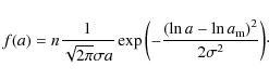
|
(1) |
Measured parameters for the particle density n, the mean particle radius
Table 2: Parameter sets for the description of maritime and continental water clouds by a log-normal distribution.
The distribution functions using these sets of parameters are
averaged according to the total ocean (![]() )
and land (
)
and land (![]() )
surface area of the Earth. The resulting mean distribution function is
used to represent low-level clouds in our climate model. We also assume
that all low-level cloud droplets are spherical particles composed of
pure liquid water. The optical properties from the obtained
distribution of the cloud particles can then be calculated with the Mie
theory (see Sect. 2.3).
)
surface area of the Earth. The resulting mean distribution function is
used to represent low-level clouds in our climate model. We also assume
that all low-level cloud droplets are spherical particles composed of
pure liquid water. The optical properties from the obtained
distribution of the cloud particles can then be calculated with the Mie
theory (see Sect. 2.3).
2.2 Size distributions of high-level cloud particles
High-level clouds represent a much more complex system, because the ice crystals can have a huge variety of shapes, which makes the description by a single distribution function and the calculation of the optical properties much more complicated. The most common shapes present in these clouds are solid and hollow columns, plates, bullets and bullet rosettes. For simplicity all ice particles are considered as solid hexagonal columns throughout this work.
Based on in-situ measurements in cirrus clouds, Heymsfield & Platt (1984)
derived analytical size distributions for high-level ice clouds using a
power law size distribution

where A is the intercept parameter, B the slope, and
| A | = | 
|
(3) |
| B | = | -3.23. | (4) |
Since the size distribution derived by Heymsfield & Platt (1984) depends only on the maximum particle dimension, we additionally need to prescribe the aspect ratio of the particles to fully describe the columns. Heymsfield (1972) provided analytical expressions for the aspect ratio
| (5) |
whereas

|
(6) |
is used for crystals with
Because the length L is always longer than the base
width D, for columns with these aspect
ratios the maximum dimension ![]() ,
which is used to parametrise the distribution function (Eq. (2)),
refers to the crystal's length in all cases.
,
which is used to parametrise the distribution function (Eq. (2)),
refers to the crystal's length in all cases.
Even assuming exclusively solid hexagonal columns as particle shapes, the calculation of the corresponding optical properties is nevertheless more complex than in the case of spherical droplets because the Mie theory cannot be applied directly. There do exist some applications for the derivation of the optical properties of these non-spherical particles, but they are either limited in their validity range (e.g. geometrical optics or ray tracing methods) or need an excessive amount of computing time (e.g. finite-time-domain theory).
However, it is possible to introduce so-called equivalent spheres, i.e. the non-spheric particles are replaced by spheres, which mimic their optical properties. In this way the Mie theory can be used again allowing a fast computation. Commonly used are equal-volume spheres and equal-area spheres, whereby a sphere has the same volume or the same surface area as the respective non-spherical particle. In both cases the number density of the equivalent spheres and the non-spherical particles remain the same, while either conserving the total volume (in the equal-volume sphere case) or the total surface area (for the equal-area sphere case) of the non-spherical particles. Still, as pointed out by Grenfell & Warren (1999), these approaches yield mostly too small scattering albedos and too large asymmetry parameters in comparison with the non-spherical particles. A much better agreement is achieved by using spheres having the same volume-to-surface ratio as the non-spherical particles (Grenfell & Warren 1999). But to conserve the total volume and area of the non-spherical particles, the number density of the equivalent spheres has to be adapted. Compared to the equal-volume or area spheres, the sizes resulting from the volume-to-surface equivalent sphere method are generally smaller, which in turn leads to smaller asymmetry parameters and larger scattering albedos. This implies that the volume-to-surface equivalent sphere approach offers a much better approximation for the calculation of the optical properties of the non-spherical particles in most cases.
The application of the volume-to-surface sphere approach for
hexagonal columns was published by Neshyba
et al. (2003). Following their treatment the radius
of the equivalent spheres for hexagonal columns is given by the
expression
|
(7) |
while the number density of the spheres

|
(8) |
As noted by Neshyba et al. (2003) these approximations have only been tested for use in energy budget studies, i.e. when using angle-averaged properties of the radiation field (e.g. the spectral flux) as done in this study (cf. 3.2). Their applicability might though be limited concerning the calculation of angle-dependent spectral intensities. In particular the required assumption of randomly oriented columns is questionable, because most of the columns are falling with their long axes parallel to the ground as confirmed by observations of e.g. Ono (1969).
2.3 Optical properties of cloud particles
For spherical particles within the size interval ![]() the usual transport coefficients are given by
the usual transport coefficients are given by
|
|
= | (9) | |
| = | (10) | ||
| = | (11) |
where
|
|
= | 
|
(12) |
| = | 
|
(13) | |
| = | 
|
(14) |
The required optical properties (extinction efficiency
|
|
= | 2 | (15) |
| = | (16) | ||
| = | (17) |
where the reflection efficiency
Instead of the full scattering phase function ![]() ,
the asymmetry parameter
,
the asymmetry parameter ![]() ,
which is defined by
,
which is defined by
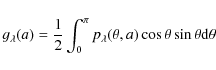
|
(18) |
for a single particle of radius a and the scattering angle
For a continuous distribution function as in the cloud description, the
average value
|
(19) |
is used, applicable for multiple scattering.
In the case of the low-level clouds we use the refractive indices for pure liquid water taken from Segelstein (1981), whereas for the high-level clouds the indices for water ice, published by Warren & Brandt (2008) are adopted. The refractive indices are assumed to be independent of temperature.
|
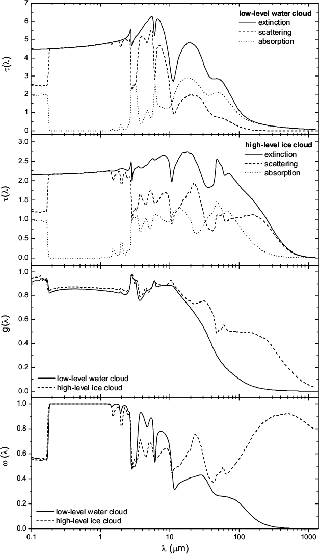
Figure 1:
Calculated optical properties of the cloud model. Upper
diagram: optical depth of the low-level water cloud (solid
line) with the individual contributions of absorption (dotted line) and
scattering (dashed line); upper middle diagram:
optical depth of the high-level ice cloud (solid line) with the
individual contributions of absorption (dotted line) and scattering
(dashed line); lower middle diagram: asymmetry
parameter |
| Open with DEXTER | |
The results of the Mie theory calculations for high- and low-level
cloud size distributions have been scaled according to the measured
optical depth from Table 1 and are shown
in Fig. 1.
Scattering dominates the radiative effects in the wavelength range
below ![]() ,
where the maximum of the incident stellar spectra is located. With a
scattering albedo of nearly
,
where the maximum of the incident stellar spectra is located. With a
scattering albedo of nearly ![]() ,
absorption is negligible in this wavelength range. Thus the clouds will
mostly scatter the incident light at short wavelengths. However, due to
high asymmetry parameters (
,
absorption is negligible in this wavelength range. Thus the clouds will
mostly scatter the incident light at short wavelengths. However, due to
high asymmetry parameters (
![]() )
much of the stellar radiation will be scattered in the forward
direction, i.e. it will still reach the planetary surface, and only a
small part is reflected back to space.
In the longer wavelengths range of the outgoing thermal radiation
around
)
much of the stellar radiation will be scattered in the forward
direction, i.e. it will still reach the planetary surface, and only a
small part is reflected back to space.
In the longer wavelengths range of the outgoing thermal radiation
around ![]() ,
the radiative effects are much more complex, because the optical
properties, especially the absorption and scattering optical depths,
show large variations.
The different effects for this case are explained in detail in
Sect. 5.1.
,
the radiative effects are much more complex, because the optical
properties, especially the absorption and scattering optical depths,
show large variations.
The different effects for this case are explained in detail in
Sect. 5.1.
3 Radiative-convective climate model
3.1 Basic assumptions
For the atmospheric model calculations we use a one-dimensional
radiative-convective climate model, which is based on the model
developed and described by Kasting
et al. (1984) and Pavlov
et al. (2000). In their atmospheric model the impact
of clouds is not explicitly treated. The effects of clouds are only
taken into account indirectly by adjusting the value of the planetary
surface albedo to mimic the influence of clouds in the troposphere.
Using the developed cloud model description (Sect. 2) we
include the climatic effects of multi-layered clouds directly into the
climate model to determine for instance the radiative feedbacks of
clouds on the surface temperature. Chemical feedbacks of clouds are not
included yet. The atmospheric profiles of the major chemical species
obtained with a detailed photochemical model (Grenfell
et al. 2007) representing the modern Earth
atmosphere are used.
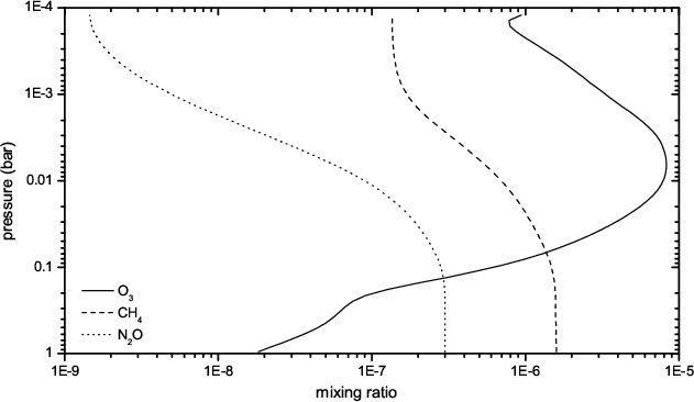
Since ![]() ,
,
![]() ,
and
,
and ![]() are well mixed within the atmosphere, their atmospheric profiles are
given by isoprofiles with mixing ratios of
are well mixed within the atmosphere, their atmospheric profiles are
given by isoprofiles with mixing ratios of ![]() ,
,
![]() and
and ![]() respectively. The profiles of
respectively. The profiles of ![]() ,
,
![]() and
and ![]() have been derived from the photochemical model for the modern Earth.
This atmospheric composition is assumed for all calculations, thereby
neglecting any change of processes influencing the chemical composition
of the planetary atmospheres, like different
have been derived from the photochemical model for the modern Earth.
This atmospheric composition is assumed for all calculations, thereby
neglecting any change of processes influencing the chemical composition
of the planetary atmospheres, like different ![]() levels due to changes in silicate weathering, for example.
levels due to changes in silicate weathering, for example.
|
Figure 2:
Atmospheric chemical profiles of |
| Open with DEXTER | |
For the relative humidity in the troposphere, from which the water profile is calculated, the empirical relative humidity distribution of Manabe & Wetherald (1967) is used. Within the troposphere the temperature is assumed to follow a moist adiabate, otherwise the temperature is calculated by the condition of radiative equilibrium. The measured Earth surface albedo of 0.13 is applied, taken from globally averaged satellite measurements of the ISCCP. The surface emission is treated as black-body radiation determined by the surface temperature.
3.2 Radiative transfer
The radiative transfer within the climate model is split into two wavelength regimes: the stellar part, dealing with the wavelength range of the incident stellar radiation and the infrared part for the treatment of the thermal radiation wavelength range.
The radiative transfer in the stellar part consists of 38
spectral intervals between ![]() and
and ![]() .
The plane-parallel equation of radiative transfer is solved by a
.
The plane-parallel equation of radiative transfer is solved by a ![]() -two-stream
quadrature method (Toon et al.
1989). Gaseous absorption of
-two-stream
quadrature method (Toon et al.
1989). Gaseous absorption of ![]() ,
,
![]() ,
,
![]() ,
,
![]() ,
and
,
and ![]() is treated with four-term correlated-k coefficients (cf. Segura et al. 2003). For
is treated with four-term correlated-k coefficients (cf. Segura et al. 2003). For
![]() ,
,
![]() and
and ![]() ,
Rayleigh scattering is also considered.
,
Rayleigh scattering is also considered.
For the IR part a hemispheric-mean two-stream method is used,
since the ![]() -two-stream
method used in the stellar part cannot be used for thermal radiation
due to numerical inaccuracies (Toon
et al. 1989). The IR radiative transfer uses 16
spectral intervals between
-two-stream
method used in the stellar part cannot be used for thermal radiation
due to numerical inaccuracies (Toon
et al. 1989). The IR radiative transfer uses 16
spectral intervals between ![]() and
and ![]() .
.
Gaseous absorption is treated with the correlated-k method
incorporated within the rapid radiative transfer model (RRTM) developed
by Mlawer et al. (1997).
Considered species in the RRTM for gaseous absorption in the IR
wavelength range are ![]() ,
,
![]() ,
,
![]() ,
,
![]() ,
and
,
and ![]() .
Scattering is neglected for gaseous species at these wavelengths. The
same approach has been used for instance by Segura
et al. (2003).
.
Scattering is neglected for gaseous species at these wavelengths. The
same approach has been used for instance by Segura
et al. (2003).
Note that the k-distributions used in the RRTM are only
tabulated over a limited pressure and temperature range. In particular
the temperature range is limited to within ![]() of an Earth mid-latitude summer temperature profile (see Mlawer et al. 1997, for
details). Beyond the tabulated range extrapolation is used to derive
the k-coefficients, which might cause inaccuracies in the upper parts
of the atmospheric temperature profiles, especially for situations
strongly deviating from (mean) Earth conditions (see also Segura
et al. 2005,2003; and von Paris et al. 2008).
of an Earth mid-latitude summer temperature profile (see Mlawer et al. 1997, for
details). Beyond the tabulated range extrapolation is used to derive
the k-coefficients, which might cause inaccuracies in the upper parts
of the atmospheric temperature profiles, especially for situations
strongly deviating from (mean) Earth conditions (see also Segura
et al. 2005,2003; and von Paris et al. 2008).
3.3 Incident stellar spectra for typical M, G, K, and F-type stars
Atmospheric calculations of Earth-like planets around different main
sequence dwarf stars, M, F, G, and K-type stars, been have published by
e.g. Kasting et al. (1993)
or Segura
et al. (2005,2003). In order to be comparable
we investigated the same stars in this study as representatives for the
different stellar types. The sample of stars used for the calculations
are the F-dwarf ![]() Bootis (HD 128167) as a typical F-type star, the Sun as the G-type
star, the young active K-type star
Bootis (HD 128167) as a typical F-type star, the Sun as the G-type
star, the young active K-type star ![]() (HD 22049), and the M-type dwarf star AD Leo (GJ 388). The basic
stellar parameters (stellar type, effective temperature
(HD 22049), and the M-type dwarf star AD Leo (GJ 388). The basic
stellar parameters (stellar type, effective temperature ![]() ,
distance of the considered star to the Sun d, and
distances from the planets to their host stars a,
for which the stellar flux matches the solar constant) with
corresponding references are shown in Table 3.
,
distance of the considered star to the Sun d, and
distances from the planets to their host stars a,
for which the stellar flux matches the solar constant) with
corresponding references are shown in Table 3.
Table 3: Properties of the different central stars.
High resolution spectra for the M-dwarf and the F-type star
were taken from Segura
et al. (2005,2003). According to Segura et al. (2003) the
F-type star spectrum is a composition from IUE satellite spectra of ![]() Bootis between
Bootis between ![]() and
and ![]() and a synthetic spectrum derived from the well-established stellar
atmosphere model of Kurucz (Kurucz 1979; Buser &
Kurucz 1992). More details on the F-star spectrum can be
found in Segura et al. (2003).
The M-type star high resolution spectrum is a composite of IUE
satellite data between
and a synthetic spectrum derived from the well-established stellar
atmosphere model of Kurucz (Kurucz 1979; Buser &
Kurucz 1992). More details on the F-star spectrum can be
found in Segura et al. (2003).
The M-type star high resolution spectrum is a composite of IUE
satellite data between ![]() and
and ![]() and an optical spectrum from Pettersen
& Hawley (1989) between
and an optical spectrum from Pettersen
& Hawley (1989) between ![]() and
and ![]() .
It was extended to
.
It was extended to ![]() in the near infrared using spectra by Leggett
et al. (1996) and a synthetic photospheric spectrum
from the stellar atmosphere model NextGen beyond
in the near infrared using spectra by Leggett
et al. (1996) and a synthetic photospheric spectrum
from the stellar atmosphere model NextGen beyond ![]() .
For further details on the M-star spectrum we refer to Segura et al. (2005).
.
For further details on the M-star spectrum we refer to Segura et al. (2005).
The K-type star spectrum is composed of IUE satellite data
from ![]() Eridani between
Eridani between ![]() and
and ![]() and a synthetic NextGen spectrum, taken from the grid of stellar
atmosphere models of France Allard
(http://perso.ens-lyon.fr/france.allard/). The high resolution spectrum
of the Sun is taken from Gueymard
(2004). This updated compilation of stellar spectra has been
used in this study.
and a synthetic NextGen spectrum, taken from the grid of stellar
atmosphere models of France Allard
(http://perso.ens-lyon.fr/france.allard/). The high resolution spectrum
of the Sun is taken from Gueymard
(2004). This updated compilation of stellar spectra has been
used in this study.
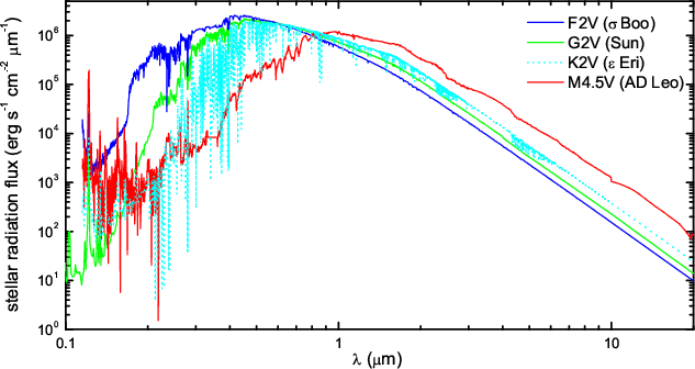
A total integrated solar radiation flux of ![]() has been derived by integration of the high resolution spectrum of Gueymard (2004) from
has been derived by integration of the high resolution spectrum of Gueymard (2004) from ![]() to
to ![]() .
In contrast to the approach of Segura et al. (2005,2003),
the distances of the four representative Earth-like extrasolar planets
to their respective central stars have been determined in this work in
a way that the integrated incident stellar flux equals this solar
constant. The corresponding orbital distances of the planets are shown
in Table 3,
and the stellar spectra of all four central stars incident at the top
of the planetary atmospheres are shown in Fig. 3.
.
In contrast to the approach of Segura et al. (2005,2003),
the distances of the four representative Earth-like extrasolar planets
to their respective central stars have been determined in this work in
a way that the integrated incident stellar flux equals this solar
constant. The corresponding orbital distances of the planets are shown
in Table 3,
and the stellar spectra of all four central stars incident at the top
of the planetary atmospheres are shown in Fig. 3.
|
Figure 3: Incident stellar spectra for different central stars. Each radiation flux is scaled to the distance where the total energy input at the top of the planetary atmosphere equals the solar constant. |
| Open with DEXTER | |
Furthermore, all four spectra have been binned to obtain the integrated
radiation fluxes required for the 38 spectral intervals from ![]() to
to ![]() used in the radiative transfer (cf. Sect. 3.2).
used in the radiative transfer (cf. Sect. 3.2).
3.4 Cloud-climate scheme
The climate model used in this work allows for a multi-layered cloud structure: two different cloud layers and the possibility of partial overlap between both layers.
The optical properties of the clouds are calculated according to the description in Sect. 2.3 and the results summarised in Fig. 1. The optical properties are assumed to be the same for all model atmospheres, i.e. no feedback of the atmospheric properties (e.g. different temperature profiles) onto the clouds is considered here. The altitude of both cloud layers is iteratively adjusted to match the measured pressure values shown in Table 1.
To account for the radiative effects of clouds, their optical
properties (optical depths, asymmetry parameter, and scattering albedo)
have been introduced into both parts of the radiative transfer scheme.
In order to account for different amounts of coverages and their
partial overlap of multi-layered clouds in our model we developed a
flux-averaging procedure. For every distinct cloud configuration i
(e.g. a low-level or a high-level cloud layer, partial overlapping
clouds etc.) and the clear sky case (![]() )
the radiative transfer is solved separately. The mean radiative flux
)
the radiative transfer is solved separately. The mean radiative flux ![]() is then determined by averaging all separately calculated fluxes
is then determined by averaging all separately calculated fluxes ![]() weighted with the corresponding cloud coverage xi
weighted with the corresponding cloud coverage xi
|
(20) |
4 Earth reference model
In order to verify the applicability of our cloud description we first
performed model calculations for the modern Earth atmosphere. ISCCP
measurements report a global mean Earth surface temperature value of ![]() ,
which we considered as reference below. Calculations for the clear sky
case and for the measured Earth mean cloud cover (39.5% low-level and
15% high-level cloud cover) have been done also considering a partial
overlap of
,
which we considered as reference below. Calculations for the clear sky
case and for the measured Earth mean cloud cover (39.5% low-level and
15% high-level cloud cover) have been done also considering a partial
overlap of ![]()
![]() between the two cloud layers. The calculated values for the surface
temperatures, the temperatures at the positions of the cloud layers,
and the Bond albedos are summarised in Table 4 and
compared to measured values taken from ISCCP data.
between the two cloud layers. The calculated values for the surface
temperatures, the temperatures at the positions of the cloud layers,
and the Bond albedos are summarised in Table 4 and
compared to measured values taken from ISCCP data.
Table 4: Summary of the different Earth reference models in comparison to measured values.
4.1 Surface temperatures
For the clear sky case, the calculated surface temperature is about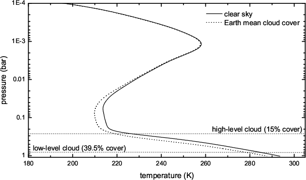
|
Figure 4: Temperature-pressure profiles of the Earth reference models. The solid line represents the clear sky case, the dotted line the model with the mean Earth cloud cover. The horizontal dashed lines represent the position of both cloud layers. |
| Open with DEXTER | |
The temperature pressure profile of the clear sky case and of the cloudy case (without overlap) are shown in Fig. 4. The positions of the two cloud layers are denoted by the two dashed lines. The profile of the model including partial overlap is not shown because it shows no noticeable difference compared to the non-overlapping case. The profiles again indicate that the clear sky calculation results in too high temperatures, while the cloudy case resembles mean Earth conditions. The presence of clouds changes the temperature profiles up through the troposphere, while the temperatures in the upper atmosphere are almost unaffected as expected.
The temperatures of the low-level clouds also agree very well
with the measured values. In contrast to that, the high-level cloud
temperatures show a difference of about ![]() in comparison to the values published by Rossow
& Schiffer (1999,
see Table 1).
Still, as was pointed out in their work, the cloud temperatures were
derived neglecting cloud IR scattering. This resulted in an
overestimate of their high-level cloud temperatures by a few degrees so
that the actual deviations of our calculated cloud temperatures are
much smaller than
in comparison to the values published by Rossow
& Schiffer (1999,
see Table 1).
Still, as was pointed out in their work, the cloud temperatures were
derived neglecting cloud IR scattering. This resulted in an
overestimate of their high-level cloud temperatures by a few degrees so
that the actual deviations of our calculated cloud temperatures are
much smaller than ![]() .
Because the optical depth and the coverage of the low-level clouds is
larger than that of high-level clouds, clouds in the present Earth
atmosphere have a net cooling effect as confirmed by our model
findings.
.
Because the optical depth and the coverage of the low-level clouds is
larger than that of high-level clouds, clouds in the present Earth
atmosphere have a net cooling effect as confirmed by our model
findings.
4.2 Bond albedo
The calculated value of 0.15 for the planetary Bond albedo (see Table 4) is much too small in the clear sky case compared with the observed Earth value of about 0.3. With clouds included in the model, the resulting Bond albedo of 0.27 (0.26 in case of overlapping clouds) agrees much better with the observed value. The remaining small difference can be explained by our neglect of the mid-level and cumulonimbus clouds, which would also contribute to the Bond albedo.
4.3 Radiative flux profiles
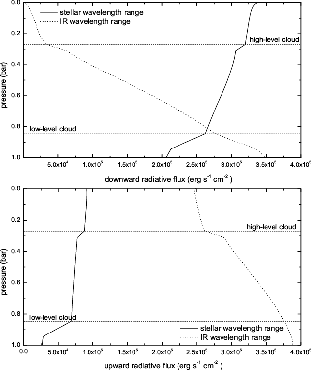
For a better understanding of the cloud radiative forcing, the upward and downward radiation flux-pressure profiles in the stellar and IR wavelengths range are shown in Fig. 5.
The downward stellar flux clearly indicates the albedo effect of both cloud layers. Due to its larger optical depth and bigger coverage, the albedo effect of the low-level cloud is much more pronounced than that of the high-level cloud. The upward infrared flux shows the blocking of the thermal radiation by the different cloud layers, i.e. the resulting greenhouse effect. The low-level cloud has almost no effect on the outgoing IR radiation and therefore exhibits no noticeable greenhouse effect. This yields a net albedo effect (see the steps in the flux profiles in Fig. 5), which leads to a cooling of the lower atmosphere and also of the planetary surface. The high-level cloud on the other hand traps more IR radiation in the lower atmosphere than it blocks the incident solar radiation. Thus, for the high-level clouds the greenhouse effect exceeds their albedo effect, which leads to a net heating in the lower atmosphere and an increase in the surface temperature (see also Fig. 7).
To summarise, our parametrised cloud model is able to reproduce the mean Earth conditions, using measured cloud properties, cloud coverages, and the Earth global mean surface albedo. The Earth reference model can reproduce the mean Earth surface temperature and the Earth Bond albedo very well. The temperatures at the cloud positions also agree favourably with measured values.
To mimic the climatic effects of clouds it is a common approach to adjust the planetary surface albedo in one-dimensional clear sky calculations (cf. e.g. Segura et al. 2003). While this approach can reproduce the correct surface temperature, these models have the shortcoming, amongst other things, that they are unable to reproduce the correct planetary Bond albedo. The parametrised cloud model, though, is able to reproduce both parameters.
5 Earth-like planetary atmospheres
|
Figure 5: Radiative flux-pressure profiles of the Earth reference calculation including clouds. The upper diagram shows the downward radiative flux in the stellar (solid line) and the IR wavelength range (dotted line), the lower diagram the upward radiative flux. The position of the two cloud layers is denoted by the horizontal dashed lines. |
| Open with DEXTER | |
|
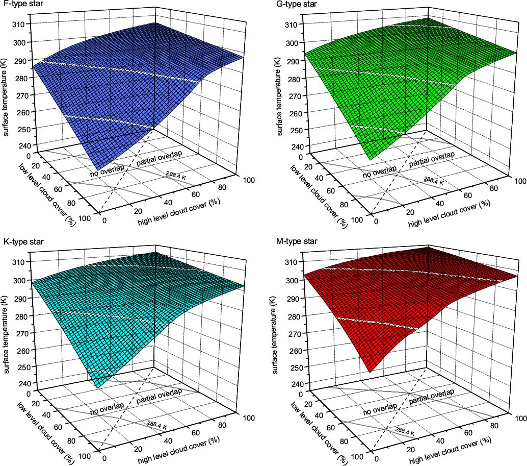
Figure 6:
Surface temperatures of planets around the four different stars
considered as a function of the cloud coverages of high and low-level
clouds. Upper left diagram: F-type star,
upper right diagram: G-type star, lower left
diagram: K-type star, lower right diagram:
M-type star. The solid lines on the contour surface and in the x-y-plane
denote the physical limits of the cloud parametrisations. The
parameters, for which a mean Earth surface temperature (
|
| Open with DEXTER | |
|
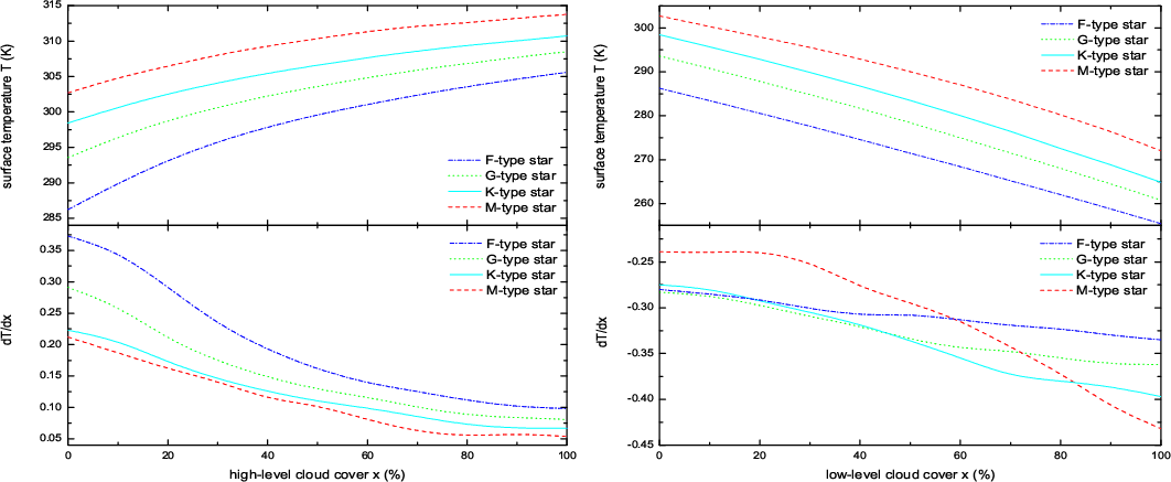
Figure 7: Basic effect of each cloud type on the surface temperatures for the four different central stars. The upper diagrams show the surface temperature as a function of the cloud coverage of the high-level cloud ( left diagram) and low-level cloud ( right diagram). The lower diagram shows the derivative of the surface temperature with respect to the cloud coverage, i.e. the change of surface temperature with cloud coverage. |
| Open with DEXTER | |
In order to quantify the climatic effects of clouds in Earth-like planetary atmospheres calculations have been carried out over the whole range of the two-dimensional parameter space of possible cloud cover combinations. For each stellar type more than 150 atmospheric models have been evaluated. The resulting surface temperatures and Bond albedos are presented in the next subsections. First implications of the position of the habitable zones of the four different central stars considered are discussed at the end of this section.
5.1 Surface temperatures
Figure 6
shows the surface temperatures as a function of the cloud coverages for
the four different central stars.
The various lines shown on the contour surfaces indicate different
regions of physical conditions. The lowest line marks the validity
range for the low-level cloud. For parameters below the corresponding
line in the x-y-plane, the
temperature of the low-level cloud drops below ![]() ,
which is the lower temperature limit for the approach (see
Sect. 2),
i.e. it represents the freezing limit for water droplet clouds. The
uppermost line on the other hand indicates the validity range of the
high-level clouds. Above that line the high-level cloud temperature is
higher than
,
which is the lower temperature limit for the approach (see
Sect. 2),
i.e. it represents the freezing limit for water droplet clouds. The
uppermost line on the other hand indicates the validity range of the
high-level clouds. Above that line the high-level cloud temperature is
higher than ![]() ,
where the ice cloud would liquefy. The middle line denotes the
parameters for which a mean Earth surface temperature of
,
where the ice cloud would liquefy. The middle line denotes the
parameters for which a mean Earth surface temperature of ![]() occurs. It should be noted that all three lines become important only
for the K and G-type stars. Due to the low resulting temperatures for
the F-type star, the limit for the high-level cloud is not reached,
while for the M-type star the temperature of the low-level cloud always
stays above
occurs. It should be noted that all three lines become important only
for the K and G-type stars. Due to the low resulting temperatures for
the F-type star, the limit for the high-level cloud is not reached,
while for the M-type star the temperature of the low-level cloud always
stays above ![]() .
.
Using the measured Earth surface albedo, results imply that
none of the four clear sky model atmospheres achieves surface
temperatures equal to the Earth mean value of ![]()
![]() . Even if the incident
stellar energy is the same for all types of stars and equals the solar
constant, the resulting clear sky surface temperatures are obviously
different (see Figs. 6, 7), which makes
the influence of the wavelength dependence of the incident radiation
quite clear, although no clouds are present and only the wavelength
dependent opacities of the gas are causing the difference in these
cases. The surface temperature of a cloudless Earth-like planet
orbiting the F-type star, for example, is lower than the measured mean
Earth surface temperature, while the other surface temperatures are
higher than
. Even if the incident
stellar energy is the same for all types of stars and equals the solar
constant, the resulting clear sky surface temperatures are obviously
different (see Figs. 6, 7), which makes
the influence of the wavelength dependence of the incident radiation
quite clear, although no clouds are present and only the wavelength
dependent opacities of the gas are causing the difference in these
cases. The surface temperature of a cloudless Earth-like planet
orbiting the F-type star, for example, is lower than the measured mean
Earth surface temperature, while the other surface temperatures are
higher than ![]() .
This is especially the case for the M-type star, which has
substantially more radiation flux in the visible and IR wavelength
regions than the other three kinds of stars (cf. Fig. 3).
Consequently clouds are required to reach
.
This is especially the case for the M-type star, which has
substantially more radiation flux in the visible and IR wavelength
regions than the other three kinds of stars (cf. Fig. 3).
Consequently clouds are required to reach ![]() in all investigated situations. Whereas the cloud layers have to
produce a net heating effect in the case of the F-type star, the albedo
effect of clouds has to be stronger than the greenhouse effect for the
other types of stars if mean Earth surface temperatures are to be
achieved under such conditions.
in all investigated situations. Whereas the cloud layers have to
produce a net heating effect in the case of the F-type star, the albedo
effect of clouds has to be stronger than the greenhouse effect for the
other types of stars if mean Earth surface temperatures are to be
achieved under such conditions.
In order to illustrate the basic climatic effect, the results
of single cloud layer calculations are shown in Fig. 7, which
summarises the corresponding slices through the 3D-temperature diagrams
of Fig. 6.
As a rule the surface temperature decreases with increasing low-level
cloud coverage, i.e. water droplet clouds exhibit a net albedo effect
for all stellar spectra. The maximum temperature decrease of about ![]() at full cloud cover is about the same for all types of central stars.
The change of the surface temperature with increasing low-level cloud
coverage is, however, not uniform. The most significant difference
appears for the M-type star, while the for the F-type star there is
almost no change in the temperature (see lower right panel of
Fig. 7).
This effect is caused by different absorption properties of the clouds
at different wavelengths in conjunction with the incident stellar
spectra. The M-star spectrum (Fig. 3) is more
extended into the IR where the frequency dependent spectral energy can
be partly absorbed by the low-level water cloud (cf. Fig. 1). In
contrast to the M-type star, the spectrum of the F-type star has its
maximum flux at a wavelength range around
at full cloud cover is about the same for all types of central stars.
The change of the surface temperature with increasing low-level cloud
coverage is, however, not uniform. The most significant difference
appears for the M-type star, while the for the F-type star there is
almost no change in the temperature (see lower right panel of
Fig. 7).
This effect is caused by different absorption properties of the clouds
at different wavelengths in conjunction with the incident stellar
spectra. The M-star spectrum (Fig. 3) is more
extended into the IR where the frequency dependent spectral energy can
be partly absorbed by the low-level water cloud (cf. Fig. 1). In
contrast to the M-type star, the spectrum of the F-type star has its
maximum flux at a wavelength range around ![]() ,
where the water cloud has an almost constant scattering albedo of about
1 (see Fig. 1),
which means that scattering dominates the radiative transfer, and the
remaining absorption has only a minor influence on the temperature.
,
where the water cloud has an almost constant scattering albedo of about
1 (see Fig. 1),
which means that scattering dominates the radiative transfer, and the
remaining absorption has only a minor influence on the temperature.
Due to their net greenhouse effect the high-level ice clouds
cause an increase in the surface temperature with increasing cloud
cover in all cases (see Fig. 7). The maximum
of the temperature increase caused by the greenhouse effect, however,
depends on the properties of the central star considered. The albedo
effect depends directly on the incident stellar spectrum, but the
greenhouse effect is determined by the thermal emission of the lower
atmosphere, which itself is an indirect consequence of the stellar
radiation. For example an Earth-like planet around the M-type star has
a maximum greenhouse effect of about ![]() at
at ![]() high-level cloud cover compared to the clear sky case. In the case of
the F-type star the greenhouse effect results in an increase of surface
temperature causing a temperature alteration of about
high-level cloud cover compared to the clear sky case. In the case of
the F-type star the greenhouse effect results in an increase of surface
temperature causing a temperature alteration of about ![]() .
In principle the greenhouse effect becomes smaller for larger
temperatures in the lower atmosphere (Fig. 7, left panel).
The effectiveness of the greenhouse effect depends directly on the
absorption characteristics of the high-level cloud in the thermal
wavelength range in conjunction with the temperature dependent infrared
emissions of the lower atmosphere.
.
In principle the greenhouse effect becomes smaller for larger
temperatures in the lower atmosphere (Fig. 7, left panel).
The effectiveness of the greenhouse effect depends directly on the
absorption characteristics of the high-level cloud in the thermal
wavelength range in conjunction with the temperature dependent infrared
emissions of the lower atmosphere.
To illustrate the absorption characteristics of the clouds as
a function of different atmospheric temperatures, we assume that the
transmission of the atmospheric layer below the cloud layer can be
represented by black-body radiation with the corresponding atmospheric
temperatures. Figure 8
shows the absorption optical depth of a high-level ice cloud with ![]() coverage in comparison to black-body radiation fluxes of different
atmospheric temperatures derived from model calculations for the four
different central stars. Compared with the other Earth-like cases, the
planet around the F-type star has the lowest atmospheric temperatures,
which results in the biggest shift of the black-body radiation to
longer wavelengths. Since the absorption at the position of the maximum
of the black-body radiation is more than
coverage in comparison to black-body radiation fluxes of different
atmospheric temperatures derived from model calculations for the four
different central stars. Compared with the other Earth-like cases, the
planet around the F-type star has the lowest atmospheric temperatures,
which results in the biggest shift of the black-body radiation to
longer wavelengths. Since the absorption at the position of the maximum
of the black-body radiation is more than ![]() smaller for the M-star than for the F-star, the greenhouse effect is
much more significant in the latter case. Thus one obtains a
temperature-induced wavelength shift for the absorbable radiation,
which results in increasing absorption and a more effective greenhouse
effect. As the temperature in the lower atmosphere increases with
larger high-level cloud cover, the maximum of the black-body radiation
is more and more shifted to smaller wavelengths which in turn decreases
the efficiency of the greenhouse effect. The amount of the greenhouse
effect is in that way self-limited. This can clearly be seen in
Fig. 7
(left lower panel) which shows the flattening of the temperature
gradients at high ice cloud coverages.
smaller for the M-star than for the F-star, the greenhouse effect is
much more significant in the latter case. Thus one obtains a
temperature-induced wavelength shift for the absorbable radiation,
which results in increasing absorption and a more effective greenhouse
effect. As the temperature in the lower atmosphere increases with
larger high-level cloud cover, the maximum of the black-body radiation
is more and more shifted to smaller wavelengths which in turn decreases
the efficiency of the greenhouse effect. The amount of the greenhouse
effect is in that way self-limited. This can clearly be seen in
Fig. 7
(left lower panel) which shows the flattening of the temperature
gradients at high ice cloud coverages.
The climatic influence of clouds in Earth-like planetary
atmospheres becomes much more complex for a multi-layered situation,
where the greenhouse effect and the albedo effect of the high and
low-level clouds are interacting non-linearly, resulting in the
3D-temperature planes displayed in Fig. 6. The
efficiency of the ice cloud greenhouse effect, for example, is much
more enhanced if a low-level cloud is present below the high-level
cloud. The albedo effect of the low-level cloud is compensated by the
ice cloud greenhouse effect. Therefore the resulting temperature
difference for increasing high-level cloud coverage is much more
pronounced at ![]() low-level cloud cover than for a single ice cloud layer. This can
clearly be inferred from Fig. 6 for all four
considered scenarios.
low-level cloud cover than for a single ice cloud layer. This can
clearly be inferred from Fig. 6 for all four
considered scenarios.

|
Figure 8:
Illustration of the efficiency of the greenhouse effect at different
atmospheric temperatures of the layer below the high-level cloud. The
solid line represents the absorption optical depth of the high-level
ice cloud. The black-body radiation fluxes for planets around the
different central stars (F-type star: dashed-dotted, G-type star:
dotted, K-type star: solid, M-type star: dashed) were scaled for
comparison. The temperatures were calculated with |
| Open with DEXTER | |
![\begin{figure}
\par\resizebox{9cm}{!}{\includegraphics[]{13491fig9.eps}}
\end{figure}](/articles/aa/full_html/2010/03/aa13491-09/img139.png)
|
Figure 9:
Effects of multi-layered clouds on the surface temperatures for the
four different central stars. The upper diagram
shows the surface temperature in dependence of the high-level cloud
coverage with |
| Open with DEXTER | |
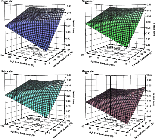
|
Figure 10:
Planetary Bond albedo of planets around the four different stars as a
function of the cloud coverages of high and low-level clouds.
Upper left diagram: F-type star, upper right
diagram: G-type star, lower left diagram:
K-type star, lower right diagram: M-type star.
Each contour square size represents a change of |
| Open with DEXTER | |
The enhancement of the greenhouse effect is, of course, a result of
lower atmospheric temperatures, reduced due to the presence of the
low-level cloud and its albedo effect. Due to the reduced temperatures
the intensity maximum of the absorbable radiation is shifted to longer
wavelengths, thereby increasing the efficiency of the greenhouse effect
(cf. Fig. 8).
The increase of the surface temperature at full
low-level cloud cover with increasing high-level cloud coverage is
shown in detail in Fig. 9,
which combines four different slices through the 3D-surface temperature
diagrams of Fig. 6,
respectively. Obviously, the temperature increase becomes weaker at
large ice cloud coverages for all cases, as also revealed by the maxima
of the corresponding temperature gradients (F-type star: ![]()
![]() ,
G-type star
,
G-type star ![]()
![]() ,
K-type star
,
K-type star ![]()
![]() ,
M-type star
,
M-type star ![]()
![]() )
shown in the lower panel of Fig. 9.
This is caused by the change of the energy transport mechanism from
radiative transfer (at smaller high-level cloud coverages) to
convection (for larger high-level cover) at the calculated heights of
the upper cloud layers in the planetary atmospheres. The switch from
convection to radiative transfer is also responsible for the second
feature in the temperature slope of the M-star planet occurring at low
ice cloud coverages. However, note that the highest (lowest) values of
the surface temperatures affected by clouds are reached for single ice
clouds (low-level clouds) with
)
shown in the lower panel of Fig. 9.
This is caused by the change of the energy transport mechanism from
radiative transfer (at smaller high-level cloud coverages) to
convection (for larger high-level cover) at the calculated heights of
the upper cloud layers in the planetary atmospheres. The switch from
convection to radiative transfer is also responsible for the second
feature in the temperature slope of the M-star planet occurring at low
ice cloud coverages. However, note that the highest (lowest) values of
the surface temperatures affected by clouds are reached for single ice
clouds (low-level clouds) with ![]() coverage (Fig. 6)
coverage (Fig. 6)![]() .
The difference between the maximum and the minimum surface temperature
again depends on the characteristics of the central star. The F-type
star causes the largest temperature variation (
.
The difference between the maximum and the minimum surface temperature
again depends on the characteristics of the central star. The F-type
star causes the largest temperature variation (![]()
![]() ), whereas the temperature
difference for the M-type star is the smallest (
), whereas the temperature
difference for the M-type star is the smallest (![]()
![]() ).
).
We note that the mean Earth surface temperature, which
requires the presence of clouds, is not uniquely obtained by one single
combination of low and high-level cloud coverages. On the contrary,
several cloud cover combinations can in principle result in a surface
temperature of ![]() as indicated by the corresponding contour lines in Fig. 6. However,
the range of coverage combinations for which mean Earth surface
conditions can be reached differs between the stellar types from the
M-type star (smallest parameter range) to the F-type star (largest
parameter range). Due to its higher incident stellar flux in the
visible and IR wavelength region, the M-type star requires a high cover
(about
as indicated by the corresponding contour lines in Fig. 6. However,
the range of coverage combinations for which mean Earth surface
conditions can be reached differs between the stellar types from the
M-type star (smallest parameter range) to the F-type star (largest
parameter range). Due to its higher incident stellar flux in the
visible and IR wavelength region, the M-type star requires a high cover
(about ![]() )
of low-level clouds as a minimum to achieve a cooling to
)
of low-level clouds as a minimum to achieve a cooling to ![]() .
For the F-type star on the other hand only about
.
For the F-type star on the other hand only about ![]() of high-level clouds are needed for the required additional heating.
of high-level clouds are needed for the required additional heating.
5.2 Bond albedo
The Bond albedo is generally an important quantity to characterise the influence and properties of clouds in planetary atmospheres. Here the Bond albedo values have been obtained for the whole two-dimensional parameter space of cloud coverages. In Fig. 10 the calculated planetary Bond albedos are shown for all four central stars considered. As expected, the albedo increases regardless of the cloud type with increasing cloud cover; i.e. in absence of any cloud the Bond albedos are given by the properties of the gas only and have very low minimal values between 0.07 for the M-type star and 0.17 for the F-type star. Overall, the albedo values for an Earth-like planet around an M-type star are lower than for the other stellar types, whereas for the F-type star the Bond albedos are the highest. This is the result of direct absorption of the incident stellar radiation by clouds and gas. Since the clouds can absorb a larger fraction of the M-star spectrum (see Figs. 1 and 3), less of that light is reflected back into space, resulting in a lower Bond albedo.
The low-level clouds have a larger impact upon the Bond
albedos than the ice clouds because their optical depth is twice as
large in the wavelength range of the stellar spectra (cf.
Figs. 1
and 3).
Therefore the Bond albedos caused by low-level clouds alone are higher
than the albedos of single ice cloud layers. One would expect that the
Bond albedos become maximal in the case of total cloud cover of both
cloud layers. This is the case for the F-, G- and K-type conditions,
whereas for the M-type star the single low-level cloud layer with ![]() coverage yields the highest Bond albedo. This is related to a slight
anomaly which is evident for the M-type star and also (but less
pronounced) for the K-type star (Fig. 10). At total
low-level cloud cover the Bond albedo starts to decrease with increasing
high-level cloud coverage. Where the ice cloud cover exceeds about
coverage yields the highest Bond albedo. This is related to a slight
anomaly which is evident for the M-type star and also (but less
pronounced) for the K-type star (Fig. 10). At total
low-level cloud cover the Bond albedo starts to decrease with increasing
high-level cloud coverage. Where the ice cloud cover exceeds about ![]() the albedo values increase again.
the albedo values increase again.
This effect can be illustrated by the radiative flux-pressure
profiles for different high-level cloud coverages and full low-level
cloud cover in the atmosphere of an Earth-like planet orbiting an
M-star (Fig. 11).
The ice cloud presence affects the downward radiative flux as expected
(upper panel of Fig. 11) by
enhanced absorption and scattering capability. But above the upper
cloud level the upward radiation flux for full ice cloud coverage is higher
than the corresponding radiation flux for only ![]() cover (see lower diagram of Fig. 11).
This can be explained by increased gas absorption of the incident
stellar radiation for these specific atmospheric conditions.
This effect deserves further investigation especially in view of
improved gas opacities.
cover (see lower diagram of Fig. 11).
This can be explained by increased gas absorption of the incident
stellar radiation for these specific atmospheric conditions.
This effect deserves further investigation especially in view of
improved gas opacities.
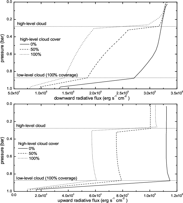
|
Figure 11:
Radiative flux-pressure profiles of different model calculations for
the M-type star to illustrate the albedo anomaly. The calculations have
been performed with a |
| Open with DEXTER | |
5.3
Habitable zone positions influenced by  clouds - first implications
The potential habitability of terrestrial planets depends on their
surface conditions, especially on the surface temperatures. Usually the
possible existence of liquid water on the planetary surface is
considered as an indication for habitable conditions. Below we refer to
the measured mean Earth surface temperature of ![]() as characteristic for the positions of habitable zones around different
kinds of central stars.
as characteristic for the positions of habitable zones around different
kinds of central stars.
As already pointed out in Sect. 3.3 the orbital
distance of the Earth-like planets to their host stars have been
determined here in a way that the incident stellar energy matches the
solar constant regardless of the atmospheric details (see
Table 3).
Using these distances, the calculated planetary surface temperatures do
not comply with the mean Earth surface temperature assuming clear sky
conditions as discussed in detail in Sect. 5.1.
Habitable conditions can yet be achieved even for these positions due
to the complex climatic effects caused by ![]() cloud layers as for the Earth for example. As previously described,
mean Earth surface temperature conditions can in principle be reached
for several cloud coverage combinations. Adjusting the stellar energy
input at the top of the atmosphere by changing the distance between the
central star and planet properly can, however also result in Earth-like
conditions for clear sky atmospheres. The deviations between these
approaches can clearly be seen in Fig. 12.
cloud layers as for the Earth for example. As previously described,
mean Earth surface temperature conditions can in principle be reached
for several cloud coverage combinations. Adjusting the stellar energy
input at the top of the atmosphere by changing the distance between the
central star and planet properly can, however also result in Earth-like
conditions for clear sky atmospheres. The deviations between these
approaches can clearly be seen in Fig. 12.
Using clear sky atmospheres the orbital distances of the
planets have to be increased (by about ![]() for the M-type star and
for the M-type star and ![]() in the case of G-type and K-type stars) to compensate for the missing
net cooling effect of the
in the case of G-type and K-type stars) to compensate for the missing
net cooling effect of the ![]() cloud layers and to achieve Earth-like conditions on the surface. For
the F-type star, the distance needs to be decreased by about
cloud layers and to achieve Earth-like conditions on the surface. For
the F-type star, the distance needs to be decreased by about ![]() ,
because in the clear sky case the surface temperature is below
,
because in the clear sky case the surface temperature is below ![]() .
Consequently, planets with a measured mean Earth cloud cover can be
located closer to the central star than planets with clear sky
atmospheres with the exception of the F-type star.
.
Consequently, planets with a measured mean Earth cloud cover can be
located closer to the central star than planets with clear sky
atmospheres with the exception of the F-type star.
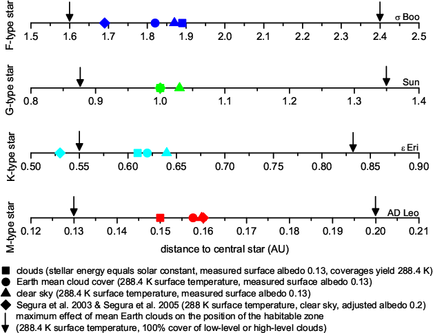
|
Figure 12: Positions of the habitable zone around different types of central stars affected by clouds. Squares mark the distances at which the incident stellar flux matches the solar constant. Circles indicate the distances for which a mean Earth surface temperature is achieved using the measured Earth cloud cover. The triangles show the positions for planets with clear sky atmospheres and a mean Earth surface temperature. The corresponding distances derived by Segura et al. (2005,2003) using a clear sky model with adjusted surface albedo are marked by diamonds. The maximum effect of the clouds on the distances are marked by arrows. |
| Open with DEXTER | |
The positions of Earth-like planets in the habitable zones calculated
by Segura
et al. (2005,2003) are also indicated in
Fig. 12
for comparison. These distances have been derived from clear sky
calculations for the Earth atmosphere with an adjusted planetary
surface albedo of 0.2 to account for the already mentioned net cooling
effect of clouds![]() and is used for all different types of central stars. Segura
et al. (2005,2003) had additionally to change
the distances of these planets to their host stars to reach a
temperature of
and is used for all different types of central stars. Segura
et al. (2005,2003) had additionally to change
the distances of these planets to their host stars to reach a
temperature of ![]() at the planetary surface even with the modified surface albedo. These
positions deviate from the distances of planets with an Earth-like
cloud cover (this work) between
at the planetary surface even with the modified surface albedo. These
positions deviate from the distances of planets with an Earth-like
cloud cover (this work) between ![]() in case of the K-type star, about
in case of the K-type star, about ![]() for the F-type star and less than
for the F-type star and less than ![]() for the M-type star. These differences are partly the consequence of
the increased surface albedo used by Segura et al. (2005,2003),
which is
for the M-type star. These differences are partly the consequence of
the increased surface albedo used by Segura et al. (2005,2003),
which is ![]() larger than the measured Earth mean value used here. A larger surface
albedo leads to less absorbed stellar flux at the surface. Therefore
the planets in the work of Segura et al. (2005,2003)
are located closer to the central star (except for the M-type star)
compared to our findings including the effect of clouds. Still, it
should be noted that other differences between the two models do also
affect the deviation in the positions of the habitable zones. An
important difference in the modelling approaches is certainly the
different treatment of the atmospheric chemistry. Here Earth-like
chemical profiles are used (see Fig. 2), whereas Segura
et al. (2005,2003) determined the chemical
composition from a photochemical model. The obvious deviation in the
case of the K-type star is mainly caused by the different stellar input
spectra used (cf. Sect. 3.3).
But apart from the well known overall effect that the positions of the
habitable zone gets closer and closer to the central star by changing
its spectral type from F to M (cf. Kasting
et al. 1993), the special spectral characteristics
of the stars are affecting the positions of the habitable zones
differently due to their complex interaction with the atmospheric cloud
layers (see Fig. 12).
larger than the measured Earth mean value used here. A larger surface
albedo leads to less absorbed stellar flux at the surface. Therefore
the planets in the work of Segura et al. (2005,2003)
are located closer to the central star (except for the M-type star)
compared to our findings including the effect of clouds. Still, it
should be noted that other differences between the two models do also
affect the deviation in the positions of the habitable zones. An
important difference in the modelling approaches is certainly the
different treatment of the atmospheric chemistry. Here Earth-like
chemical profiles are used (see Fig. 2), whereas Segura
et al. (2005,2003) determined the chemical
composition from a photochemical model. The obvious deviation in the
case of the K-type star is mainly caused by the different stellar input
spectra used (cf. Sect. 3.3).
But apart from the well known overall effect that the positions of the
habitable zone gets closer and closer to the central star by changing
its spectral type from F to M (cf. Kasting
et al. 1993), the special spectral characteristics
of the stars are affecting the positions of the habitable zones
differently due to their complex interaction with the atmospheric cloud
layers (see Fig. 12).
The maximum effect of mean Earth clouds on the position of the
habitable zone are denoted by arrows in Fig. 12. These
distances have been derived with ![]() of either cloud type while still obtaining a mean Earth surface
temperature of
of either cloud type while still obtaining a mean Earth surface
temperature of ![]() .
Using low-level clouds for a maximum cooling effect, the planets can be
located up to
.
Using low-level clouds for a maximum cooling effect, the planets can be
located up to ![]() closer to the central star compared to a clear sky planet. The
distances can be increased by up to
closer to the central star compared to a clear sky planet. The
distances can be increased by up to ![]() when single high-level cloud layers are present. The distances derived
by Segura
et al. (2005,2003) are in all cases within
these boundaries, except for the already discussed K-type star.
when single high-level cloud layers are present. The distances derived
by Segura
et al. (2005,2003) are in all cases within
these boundaries, except for the already discussed K-type star.
It is important to note that the distances derived in this
work are only indications of the position of the habitable zone, they
do not indicate its boundaries![]() .
The inner boundary is determined by the runaway greenhouse effect while
the outer edge is determined by
.
The inner boundary is determined by the runaway greenhouse effect while
the outer edge is determined by ![]() clouds (cf. Kasting 1988;
and Selsis et al. 2007).
Since these kinds of atmospheres are in general far from being
Earth-like, our parametrised cloud description, which is based on
measurements in the Earth atmosphere, is unsuitable to study the
effects of clouds on the boundaries of the habitable zone. Further
studies of the effects of clouds on habitable zones require therefore a
cloud microphysics model to evaluate the cloud properties (e.g. optical
thickness, wavelength dependent optical properties, altitude) properly,
since measurements and therefore also parametrised descriptions of them
are not available for these more extreme physical conditions.
A more detailed analysis of the influence of clouds on the position and
extension of the habitable zone will be addressed in a forthcoming
publication.
clouds (cf. Kasting 1988;
and Selsis et al. 2007).
Since these kinds of atmospheres are in general far from being
Earth-like, our parametrised cloud description, which is based on
measurements in the Earth atmosphere, is unsuitable to study the
effects of clouds on the boundaries of the habitable zone. Further
studies of the effects of clouds on habitable zones require therefore a
cloud microphysics model to evaluate the cloud properties (e.g. optical
thickness, wavelength dependent optical properties, altitude) properly,
since measurements and therefore also parametrised descriptions of them
are not available for these more extreme physical conditions.
A more detailed analysis of the influence of clouds on the position and
extension of the habitable zone will be addressed in a forthcoming
publication.
6 Summary
We developed a parametrised cloud description scheme for Earth-like planetary atmospheres based on measurements of clouds in the Earth's atmosphere. The optical properties of the clouds were calculated with the Mie theory combined with an equivalent sphere approach for the ice crystals. This cloud scheme was coupled with a one-dimensional radiative convective climate model, and its applicability was tested on an Earth reference model. Model calculations were made for Earth-like planetary atmospheres of planets orbiting different types of main sequence dwarf stars: F, G, K, and M-type stars.
It was shown that the albedo effect is only weakly dependent on the incident stellar spectra because the optical properties (especially the scattering albedo) remain almost constant in the wavelength range of the maximum of the incident stellar radiation. The greenhouse effect of the high-level cloud on the other hand depends on the temperatures of the lower atmosphere, which in turn are an indirect consequence of the different types of central stars. The efficiency of the greenhouse effect increases with smaller temperatures in the lower atmosphere and decreases with higher atmospheric temperatures. As a rule the planetary Bond albedos increase with cloud cover of either cloud type. However, for the K and M-type star an anomaly was found resulting in a decreasing Bond albedo with increasing cloud cover for a certain region in the parameter space. This anomaly is caused by enhanced gas absorption under these specific atmospheric conditions.
Planets with Earth-like clouds in their atmospheres can be located closer to the central star or farther away compared to planets with clear sky atmospheres. The change in distance depends on the type of cloud. In general, low-level clouds result in a decrease of distance because of their albedo effect, while the high-level clouds lead to an increase in distance.
Apart from these climatic effects, clouds also affect the planetary emission and transmission spectra, which is important concerning the detectability of spectral signatures of e.g. biomarker molecules. The investigation of the influence of clouds on these effects will be done in further studies.
AcknowledgementsThis work has been partly supported by the Forschungsallianz Planetary Evolution and Life of the Helmholtz Gemeinschaft (HGF).
References
- Bohren, C. F., & Huffman, D. R. 1983, Absorption and Scattering of Light by Small Particles (New York: John Wiley & Sons) [Google Scholar]
- Buser, R., & Kurucz, R. 1992, A&A, 264, 557 [NASA ADS] [Google Scholar]
- Cenarro, A. J., Peletier, R. F., Sanchez-Blazquez, P., et al. 2007, VizieR Online Data Catalog, 837, 40664 [NASA ADS] [Google Scholar]
- Cox, A. N. 2000, Allen's Astrophysical Quantities (New York: Springer) [Google Scholar]
- Grenfell, J. L., Stracke, B., von Paris, P., et al. 2007, Planet. Space Sci., 55, 661 [NASA ADS] [CrossRef] [Google Scholar]
- Grenfell, T. C., & Warren, S. G. 1999, J. Geophys. Res., 104, 31 697 [Google Scholar]
- Gueymard, C. A. 2004, Solar Energy, 76, 423 [NASA ADS] [CrossRef] [Google Scholar]
- Habing, H. J., Dominik, C., Jourdain de Muizon, M., et al. 2001, A&A, 365, 545 [NASA ADS] [CrossRef] [EDP Sciences] [Google Scholar]
- Heymsfield, A. 1972, J. Atmos. Sci., 29, 1348 [NASA ADS] [CrossRef] [Google Scholar]
- Heymsfield, A., & Platt, C. M. R. 1984, J. Atmos. Sci., 41, 846 [NASA ADS] [CrossRef] [Google Scholar]
- Kaltenegger, L., Traub, W. A., & Jucks, K. W. 2007, ApJ, 658, 598 [NASA ADS] [CrossRef] [Google Scholar]
- Kasting, J. F. 1988, Icarus, 74, 472 [NASA ADS] [CrossRef] [PubMed] [Google Scholar]
- Kasting, J. F., Pollack, J. B., & Ackerman, T. P. 1984, Icarus, 57, 335 [NASA ADS] [CrossRef] [Google Scholar]
- Kasting, J. F., Whitmire, D. P., & Reynolds, R. T. 1993, Icarus, 101, 108 [NASA ADS] [CrossRef] [PubMed] [Google Scholar]
- Kokhanovsky, A. A. 2006, Cloud Optics (Dordrecht: Springer) [Google Scholar]
- Kondratyev, K. Y. 1999, Climatic Effects of Aerosols and Clouds (Heidelberg: Springer) [Google Scholar]
- Kurucz, R. 1979, ApJS, 40, 1 [NASA ADS] [CrossRef] [Google Scholar]
- Leggett, S. K., Allard, F., Berriman, G., Dahn, C. C., & Hauschildt, P. H. 1996, ApJS, 104, 117 [NASA ADS] [CrossRef] [EDP Sciences] [Google Scholar]
- Manabe, S., & Wetherald, R. T. 1967, J. Atmos. Sci., 24, 241 [Google Scholar]
- McFarquhar, G. M., & Heymsfield, A. J. 1998, J. Atmos. Sci., 55, 2039 [NASA ADS] [CrossRef] [Google Scholar]
- Mitchell, D. L. 2002, J. Atmos. Sci., 59, 2330 [NASA ADS] [CrossRef] [Google Scholar]
- Mlawer, E. J., Taubman, S. J., Brown, P. D., Iacono, M. J., & Shepard, A. C. 1997, J. Geophys. Res., 102, 16 663 [Google Scholar]
- Neshyba, S. P., Grenfell, T. C., & Warren, S. G. 2003, J. Geophys. Res., 108, 4448 [CrossRef] [Google Scholar]
- Ono, A. 1969, J. Atmos. Sci., 26, 138 [NASA ADS] [CrossRef] [Google Scholar]
- Pavlov, A. A., Kasting, J. F., & Brown, L. L. 2000, J. Geophys. Res., 105, 11 981 [Google Scholar]
- Pettersen, B. R., & Hawley, S. L. 1989, A&A, 217, 187 [NASA ADS] [Google Scholar]
- Poetzsch-Heffter, C., Liu, Q., Ruprecht, E., & Simmer, C. 1995, J. Climate, 8, 829 [NASA ADS] [CrossRef] [Google Scholar]
- Pruppacher, H. R., & Klett, J. D. 1997, Microphysics of Clouds and Precipitation (Dordrecht: Kluwer Academic Publishers) [Google Scholar]
- Rossow, W. B., & Schiffer, R. A. 1999, Bull. Amer. Met. Soc., 80, 2261 [Google Scholar]
- Santos, N. C., Israelian, G., & Mayor, M. 2004, A&A, 415, 1153 [NASA ADS] [CrossRef] [EDP Sciences] [Google Scholar]
- Segelstein, D. 1981, Master's thesis, University of Missouri - Kansas City [Google Scholar]
- Segura, A., Krelove, K., Kasting, J. F., et al. 2003, Astrobiology, 3, 689 [Google Scholar]
- Segura, A., Kasting, J. F., Meadows, V., et al. 2005, Astrobiology, 5, 706 [NASA ADS] [CrossRef] [PubMed] [Google Scholar]
- Selsis, F., Kasting, J. F., Levrard, B., et al. 2007, A&A, 476, 1373 [NASA ADS] [CrossRef] [EDP Sciences] [Google Scholar]
- Toon, O. B., Mckay, C. P., & Ackerman, T. P. 1989, J. Geophys. Res., 94, 16 287 [Google Scholar]
- von Paris, P., Rauer, H., Grenfell, J. L., et al. 2008, Planet. Space Sci., 56, 1244 [NASA ADS] [CrossRef] [Google Scholar]
- Warren, S. G., & Brandt, R. E. 2008, J. Geophys. Res., 26, D14220 [Google Scholar]
- Warren, S. G., Eastman, R. M., & Hahn, C. J. 2007, J. Climate, 20, 717 [Google Scholar]
Footnotes
- ...

![[*]](/icons/foot_motif.png)
- This is of course the reason why the surface albedo has to be adjusted to mimic the effect of clouds in clear sky model calculations for Earth.
- ...)
- The applicability limitations of the cloud description should thereby be kept in mind.
- ... clouds
- This tuning, however, is only possible if the target surface temperature is prescribed, while in case of the model including clouds the surface temperature is a result of the calculations.
- ... boundaries
- See e.g. Selsis et al. (2007) for a study on the boundaries of the habitable zone of planets around different types of central stars.
All Tables
Table 1: Mean cloud properties obtained from surface and satellite measurements.
Table 2: Parameter sets for the description of maritime and continental water clouds by a log-normal distribution.
Table 3: Properties of the different central stars.
Table 4: Summary of the different Earth reference models in comparison to measured values.
All Figures
|
|
Figure 1:
Calculated optical properties of the cloud model. Upper
diagram: optical depth of the low-level water cloud (solid
line) with the individual contributions of absorption (dotted line) and
scattering (dashed line); upper middle diagram:
optical depth of the high-level ice cloud (solid line) with the
individual contributions of absorption (dotted line) and scattering
(dashed line); lower middle diagram: asymmetry
parameter |
| Open with DEXTER | |
| In the text | |
|
|
Figure 2:
Atmospheric chemical profiles of |
| Open with DEXTER | |
| In the text | |
|
|
Figure 3: Incident stellar spectra for different central stars. Each radiation flux is scaled to the distance where the total energy input at the top of the planetary atmosphere equals the solar constant. |
| Open with DEXTER | |
| In the text | |
|
|
Figure 4: Temperature-pressure profiles of the Earth reference models. The solid line represents the clear sky case, the dotted line the model with the mean Earth cloud cover. The horizontal dashed lines represent the position of both cloud layers. |
| Open with DEXTER | |
| In the text | |
|
|
Figure 5: Radiative flux-pressure profiles of the Earth reference calculation including clouds. The upper diagram shows the downward radiative flux in the stellar (solid line) and the IR wavelength range (dotted line), the lower diagram the upward radiative flux. The position of the two cloud layers is denoted by the horizontal dashed lines. |
| Open with DEXTER | |
| In the text | |
|
|
Figure 6:
Surface temperatures of planets around the four different stars
considered as a function of the cloud coverages of high and low-level
clouds. Upper left diagram: F-type star,
upper right diagram: G-type star, lower left
diagram: K-type star, lower right diagram:
M-type star. The solid lines on the contour surface and in the x-y-plane
denote the physical limits of the cloud parametrisations. The
parameters, for which a mean Earth surface temperature (
|
| Open with DEXTER | |
| In the text | |
|
|
Figure 7: Basic effect of each cloud type on the surface temperatures for the four different central stars. The upper diagrams show the surface temperature as a function of the cloud coverage of the high-level cloud ( left diagram) and low-level cloud ( right diagram). The lower diagram shows the derivative of the surface temperature with respect to the cloud coverage, i.e. the change of surface temperature with cloud coverage. |
| Open with DEXTER | |
| In the text | |
|
|
Figure 8:
Illustration of the efficiency of the greenhouse effect at different
atmospheric temperatures of the layer below the high-level cloud. The
solid line represents the absorption optical depth of the high-level
ice cloud. The black-body radiation fluxes for planets around the
different central stars (F-type star: dashed-dotted, G-type star:
dotted, K-type star: solid, M-type star: dashed) were scaled for
comparison. The temperatures were calculated with |
| Open with DEXTER | |
| In the text | |
|
|
Figure 9:
Effects of multi-layered clouds on the surface temperatures for the
four different central stars. The upper diagram
shows the surface temperature in dependence of the high-level cloud
coverage with |
| Open with DEXTER | |
| In the text | |
|
|
Figure 10:
Planetary Bond albedo of planets around the four different stars as a
function of the cloud coverages of high and low-level clouds.
Upper left diagram: F-type star, upper right
diagram: G-type star, lower left diagram:
K-type star, lower right diagram: M-type star.
Each contour square size represents a change of |
| Open with DEXTER | |
| In the text | |
|
|
Figure 11:
Radiative flux-pressure profiles of different model calculations for
the M-type star to illustrate the albedo anomaly. The calculations have
been performed with a |
| Open with DEXTER | |
| In the text | |
|
|
Figure 12: Positions of the habitable zone around different types of central stars affected by clouds. Squares mark the distances at which the incident stellar flux matches the solar constant. Circles indicate the distances for which a mean Earth surface temperature is achieved using the measured Earth cloud cover. The triangles show the positions for planets with clear sky atmospheres and a mean Earth surface temperature. The corresponding distances derived by Segura et al. (2005,2003) using a clear sky model with adjusted surface albedo are marked by diamonds. The maximum effect of the clouds on the distances are marked by arrows. |
| Open with DEXTER | |
| In the text | |
Copyright ESO 2010
Current usage metrics show cumulative count of Article Views (full-text article views including HTML views, PDF and ePub downloads, according to the available data) and Abstracts Views on Vision4Press platform.
Data correspond to usage on the plateform after 2015. The current usage metrics is available 48-96 hours after online publication and is updated daily on week days.
Initial download of the metrics may take a while.