| Issue |
A&A
Volume 511, February 2010
|
|
|---|---|---|
| Article Number | A26 | |
| Number of page(s) | 8 | |
| Section | Extragalactic astronomy | |
| DOI | https://doi.org/10.1051/0004-6361/200912966 | |
| Published online | 26 February 2010 | |
Retardation of non-thermal photon light curves from flaring blazars
I. Synchrotron radiation
B. Eichmann1,2 - R. Schlickeiser1 - W. Rhode2
1 - Institut für Theoretische Physik, Lehrstuhl IV:
Weltraum- und Astrophysik, Ruhr-Universität Bochum, 44780 Bochum, Germany
2 -
Experimentelle Physik V, Technische Universität Dortmund, 44221 Dortmund, Germany
Received 23 July 2009 / Accepted 28 November 2009
Abstract
An analytical model is presented which describes the intrinsic synchrotron intensity emitted by
a spherical plasmoid volume of radius R in the jet of an active galactic nucleus (AGN). Analytical results
for the emergent synchrotron intensity could be achieved by using a monochromatic approximation
for the synchrotron power. The synchrotronintensity is given by an infinite
sum, reflecting the spatial eigenfunction distribution of the radiating electrons over the
emission knot. The radiative transport of the generated synchrotronphotons is simplified
by the use of the escape probability concept which approximates the spatial
photon diffusion caused by multiple Compton scatterings off thermal electrons in the knot.
With these assumptions conclusions on the total duration of the synchrotron flare, its starting time and the cause for
even shorter time variabilities are derived. The total flare duration at all photon energies ![]() equals the
light travel time 2R/c. Shorter photon energy-dependent synchrotronintensity time variations are possible,
which reflect the influence of the photon retardation and escape as well as the temporal and spatial dependences
of the relativistic electron density distribution. The starting time of the synchrotron flare
is delayed with respect to the injection time of ultrarelativistic electrons t0 by a photon energy
dependent time scale
equals the
light travel time 2R/c. Shorter photon energy-dependent synchrotronintensity time variations are possible,
which reflect the influence of the photon retardation and escape as well as the temporal and spatial dependences
of the relativistic electron density distribution. The starting time of the synchrotron flare
is delayed with respect to the injection time of ultrarelativistic electrons t0 by a photon energy
dependent time scale
![]() ,
reflecting the necessary cooling time
which relativistic electrons need in order to radiate at photon energies below the initial characteristic
synchrotronphoton energy E0.
,
reflecting the necessary cooling time
which relativistic electrons need in order to radiate at photon energies below the initial characteristic
synchrotronphoton energy E0.
Key words: radiation mechanisms: non-thermal - galaxies: active - gamma rays: galaxies
1 Introduction
The recently launched AGILE and FERMI satellite mission together with new generation of ground-based air Cherenkov telescopes such as HESS, VERITAS and MAGIC provide unprecedented accurate coverage of our universe at GeV to TeV photon energies. The nearly all-sky field-of-view of FERMI and the much improved sensitivity of the air Cherenkov telescopes open up new opportunities to investigate especially powerful variable high-energy photon emitters such as active galactic nuclei (AGNs). The air Cherenkov telescopes have detected 27 AGNs as powerful variable high-energy photon emitters: apart from the radio galaxies M 87, Cen A and 3C 66B each of them belong to the blazar class which is characterized by rapid time variability at all wavelengths. These blazars often have established superluminal motion components at radio and mm frequencies. For strong enough flaring blazar sources at cosmological distances such as PKS 2155-304 (redshift z=0.116) (Aharonian et al. 2007) and Mrk 421 (z=0.030) (Woo et al. 2005; Albert et al. 2007) the observed high fluxes now allow the determination of accurate photon spectra and light curves from MeV to TeV energies on time scales of minutes, often supplemented by dedicated time-correlated observations at lower radio to X-ray photon energies. These detailed observations allow us to perform crucial tests of our current understanding of the physical processes responsible for the generation of intense variable non-thermal radiation in these sources. In particular, it will be possible to determine the primary hadronic or leptonic nature of non-thermal radiation production in these sources, which is closely related to the question of the nature of cosmic particle accelerators, one of the eleven open fundamental problems of physics for the new millenium (Turner et al. 2003).
The combination of high observed luminosities with the observed short time variability in blazar flares indicates that the photon emission in blazars originates in relativistic jet knots that are beamed and Doppler-boosted towards the observer (e.g. Schlickeiser 1996). Superluminal expansions observed with VLBI (Piner & Edwards 2004) provide evidence for moderate Doppler boosting factors in PKS 2155-304, although the TeV variability time scales require the presence of much larger Doppler factors in these jets. The properties of the observed non-thermal radiation from relativistic moving jet emission components are determined by intrinsic charged particle acceleration processes (intrinsic processes), environmental conditions causing high or low luminosity, external (to the jet) target photon fields, and Doppler boosting of beamed intensities and frequencies depending on the observer's viewing angle with respect to the direction of motion of the jet components (geometry influence).
The broadband continuum spectra of blazars are dominated by non-thermal emission and often
consist of two distinct broad components. While there is considerable debate concerning the nature of the
high energy spectral component (decay of neutral pions in hadronic emission models versus
inverse Compton scattering of intrinsic (SSC) and external low-energy photons in leptonic
emission models), it is agreed that the low-energy component is synchrotron radiation from highly
relativistic electrons. The peak of the low-frequency flux density component is caused by
the transition from optically thick to optically thin synchrotronradiation, and is located during the
time of maximum ![]() -ray emission at infrared to optical frequencies. Only after considerable source
expansion do these emission knots become optically thin at radio frequencies, where we can measure
superluminal expansion speeds with VLBI techniques.
-ray emission at infrared to optical frequencies. Only after considerable source
expansion do these emission knots become optically thin at radio frequencies, where we can measure
superluminal expansion speeds with VLBI techniques.
To model the multiwavelength flaring behaviour of blazars we consider a one-zone
spherical (size
R=1015R15 cm), partly turbulent magnetised (field strength B=1b Gauss) emission
knot, containing a non-relativistic plasma of electrons and ions (or positrons) of a density
Nb=1010N10 cm-3, which moves with the relativistic speed ![]() in a direction
in a direction ![]() with respect to the observer, so that the Doppler factor
with respect to the observer, so that the Doppler factor
![]() applies to the Lorentz transformation of intensities
and time scales from the coordinate system comoving with the emission knot to the observer's frame (see Appendix
B for details). Multiple Compton scatterings of the generated synchrotronphotons with optical depth
applies to the Lorentz transformation of intensities
and time scales from the coordinate system comoving with the emission knot to the observer's frame (see Appendix
B for details). Multiple Compton scatterings of the generated synchrotronphotons with optical depth
![]() ,
where
,
where
![]() is the Thomson cross section, then allow one to
use the diffusion approximation for the spatial transport of synchrotronphotons (Sunyaev & Titarchuk 1980, 1985),
implying a nearly isotropic synchrotronphoton density distribution over the emission knot.
The study represented here therefore is for an emission knot that is Thomson-thick from non-relativistic
plasma. Such a high number density of non-relativistic background particles is
needed in hadronic emission models for the jet emission (Pohl & Schlickeiser 2000) to generate
enough pions from inelastic hadron-hadron conditions. Moreover, an optical depth greater than unity for
multiple Compton scattering of synchrotron photons in the knot justifies the diffusion approximation to the
synchrotron photon transport considered below and the small anisotropy of the radiation field near the edge of the
emission knot.
is the Thomson cross section, then allow one to
use the diffusion approximation for the spatial transport of synchrotronphotons (Sunyaev & Titarchuk 1980, 1985),
implying a nearly isotropic synchrotronphoton density distribution over the emission knot.
The study represented here therefore is for an emission knot that is Thomson-thick from non-relativistic
plasma. Such a high number density of non-relativistic background particles is
needed in hadronic emission models for the jet emission (Pohl & Schlickeiser 2000) to generate
enough pions from inelastic hadron-hadron conditions. Moreover, an optical depth greater than unity for
multiple Compton scattering of synchrotron photons in the knot justifies the diffusion approximation to the
synchrotron photon transport considered below and the small anisotropy of the radiation field near the edge of the
emission knot.
Note that below all physical quantities in the observer's frame are denoted by an asterisk. A chaotic magnetic field of a constant strength B is adopted, which is randomly oriented on scales much larger than the gyroradii of the injected ultrarelativistic particles, so that classical angle-averaged synchrotron radiation formulae can be used (Crusius & Schlickeiser 1986, 1988).
After accounting for the Doppler time dilatation, the
intrinsic variability time scale
![]() of radiation is caused by five different physical processes:
of radiation is caused by five different physical processes:
- (1)
- the injection of the radiating relativistic particles in the emission knot due to acceleration or energisation processes;
- (2)
- the spatial diffusion of the injected relativistic particles in the emission knot resulting from pitch-angle scattering in the partly turbulent and chaotic magnetic field;
- (3)
- the radiative cooling of relativistic particles;
- (4)
- the spatial escape of the generated non-thermal photons in the emission knot resulting from multiple Compton scattering off the cold electrons; and
- (5)
- effects due to causality and retardation relating generated photon number densities inside the emission blob to the photon density at the edge R of the emission blob from where they can escape freely.
It is the purpose of the present paper to extend the SR-analysis by including
the effects due to the spatial propagation of relativistic electrons (2) as well as photon propagation (4)
and retardation (5), which arise due to the finite size of the emission knot. Our goal is to disentangle
the variability effects caused by radiative cooling of the relativistic electrons from
propagation and retardation effects. SR have found that at the optical, UV, X-ray and ![]() -ray
photon frequency bands optical thickness effects due to synchrotron
self absorption are negligible. We will therefore restrict our
discussion of photon propagation to the optically thin regime. Because
of the complexity of the subject, we limit our analysis here to the
variability of synchrotronradiation, whereas the variability of inverse
Compton radiation (synchrotron-self-Compton and external Compton) will
be addressed in future work.
-ray
photon frequency bands optical thickness effects due to synchrotron
self absorption are negligible. We will therefore restrict our
discussion of photon propagation to the optically thin regime. Because
of the complexity of the subject, we limit our analysis here to the
variability of synchrotronradiation, whereas the variability of inverse
Compton radiation (synchrotron-self-Compton and external Compton) will
be addressed in future work.
The organisation of the paper is as follows: in Sects. 2 and 3 we discuss and solve the
time-dependent evolution of the kinetic equations for the densities of
radiating relativistic electrons (
![]() )
and for the non-thermal synchrotron photons
(
)
and for the non-thermal synchrotron photons
(
![]() ), neglecting absorption inside the emission knot.
Because the spatial electron diffusion operator is of the Sturm-Liouville type, the solutions are
obtained by expanding with respect to the self-adjoint diffusion eigenfunctions. The full radial dependence
of the synchrotron photon density over the cloud is needed to account for the retardation effect.
The emergent intrinsic synchrotron photon intensity is proportional to the synchrotronphoton density
), neglecting absorption inside the emission knot.
Because the spatial electron diffusion operator is of the Sturm-Liouville type, the solutions are
obtained by expanding with respect to the self-adjoint diffusion eigenfunctions. The full radial dependence
of the synchrotron photon density over the cloud is needed to account for the retardation effect.
The emergent intrinsic synchrotron photon intensity is proportional to the synchrotronphoton density
![]() at the edge of the emission cloud, calculated in Sect. 4. For illustrative examples
of the spatial variation of the ultrarelativistic electron injection rate, we calculate in Sect. 5
the resulting emergent synchrotron intensities.
at the edge of the emission cloud, calculated in Sect. 4. For illustrative examples
of the spatial variation of the ultrarelativistic electron injection rate, we calculate in Sect. 5
the resulting emergent synchrotron intensities.
2 Kinetic equations of photons and electrons
All physical quantities are calculated in a coordinate system comoving with the radiation source.
2.1 Relativistic electrons
The differential number density of relativistic electrons
![]() obeys the transport equation
(with the relativistic electron Lorentz factor
obeys the transport equation
(with the relativistic electron Lorentz factor
![]() )
)
![\begin{displaymath}{\partial n\over \partial t}={1\over r^2}{\partial \over \par...
...}\left[\vert\dot{\gamma }\vert n\right]+q_1(\gamma ,t)q_2(r) ,
\end{displaymath}](/articles/aa/full_html/2010/03/aa12966-09/img16.png)
where the spatial diffusion is caused by rapid pitch-angle scattering in the partly turbulent chaotic magnetic field of the emission knot (Schlickeiser et al. 2002; Stockem & Schlickeiser 2007). We adopt a constant diffusion coefficient
in terms of the mean scattering length l0. We also adopt a separable source term of relativistic electrons
![\begin{displaymath}\vert\dot{\gamma }\vert=D_{\rm s}\gamma ^2,\;\;
D_{\rm s}={4...
...^{-14}\left[{U_B\over m_{\rm e}c^2}\right] \;~~ \hbox{s}^{-1}.
\end{displaymath}](/articles/aa/full_html/2010/03/aa12966-09/img19.png)
The particle transport Eq. (1) then reads
![\begin{displaymath}{\partial n\over \partial t}={cl_0\over 3r^2}{\partial \over ...
... }\left[\vert\dot{\gamma }\vert n\right]+q_1(\gamma ,t)q_2(r).
\end{displaymath}](/articles/aa/full_html/2010/03/aa12966-09/img20.png)
The spatial boundary conditions for electron propagation are
- (a)
- finite density
 at the centre of the knot; and
- (b)
- no particle flux from outside onto the boundary surface of the spherical knot:
implying
![\begin{displaymath}\left[D_0{\partial n\over \partial r}+{c\over 2}n\right]_{r=R...
...r 3}{\partial n\over \partial r}+{c\over 2}n\right]_{r=R}=0~ ,
\end{displaymath}](/articles/aa/full_html/2010/03/aa12966-09/img22.png)
![\begin{displaymath}\left[{\partial n\over \partial r}+{3\over 2l_0}n\right]_{r=R}=0
.
\end{displaymath}](/articles/aa/full_html/2010/03/aa12966-09/img23.png)
2.2 Photon retardation
The relativistic electrons emit photons isotropically at every point
![]() within the
spherically-symmetric source where r,
within the
spherically-symmetric source where r, ![]() and
and
![]() denote the photon's spherical coordinates.
Let
denote the photon's spherical coordinates.
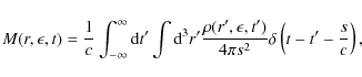
Let
![]() denote the omnidirectional photon production rate per unit volume at a time t' and a distance r' from the centre
of the source. If the source is optically thin, then the photon density at a time t, a distance r and
an energy
denote the omnidirectional photon production rate per unit volume at a time t' and a distance r' from the centre
of the source. If the source is optically thin, then the photon density at a time t, a distance r and
an energy ![]() is given by integrating over all emission points inside the source, generalising Gould's (1979)
formula for non-stationary sources:
is given by integrating over all emission points inside the source, generalising Gould's (1979)
formula for non-stationary sources:
with the distance
![$\displaystyle \times\sqrt{1-\mu ^{'2}}\cos (\phi -\phi')\bigr]\Bigr)^{1/2}.$](/articles/aa/full_html/2010/03/aa12966-09/img31.png)
Because of the spherical symmetry of the problem we can choose the spherical coordinates in a way that
so that Eq. (7) becomes
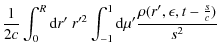
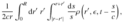
where we substituted s from Eq. (9) for the variable
At the source surface r=R the photon intensity is then given by
When the surface of the emission cloud is reached, the photons can propagate freely to the observer. The emergent photon intensity therefore equals the surface intensity
If the emission cloud propagates itself with relativistic speed
at an angle ![]() with respect to the observer, a proper Lorentz transformation of the photon intensity and
the photon energy to the observer's frame has to be applied.
with respect to the observer, a proper Lorentz transformation of the photon intensity and
the photon energy to the observer's frame has to be applied.
The omnidirectional photon production rate is related to the spontaneous photon emission coefficient by
where the exponential factor makes use of the escape probability concept of Lightman & Zdziarski (1987) and Coppi (1992). Here
![$\displaystyle ~= \left\{
\begin{array}{lll}
1 & \quad\textrm{for}&\quad x\le 0....
...quad 0.1< x <1 \\ [1mm]
0 & \quad\textrm{for}&\quad x\ge 1,
\end{array}\right.$](/articles/aa/full_html/2010/03/aa12966-09/img46.png)
and
![$\displaystyle {3\sigma _{\rm T}\over 8x}
\left[{4\over x}+{2x(1+x)\over (1+2x)^2}-{2+2x-x^2\over x^2}\ln (1+2x)\right]$](/articles/aa/full_html/2010/03/aa12966-09/img50.png)
![$\displaystyle \left\{
\begin{array}{lll}
\sigma _{\rm T} &\quad \textrm{for}& x...
...rm T}\over 16x}[1+2\ln (2x)] & \quad\textrm{for} & x\gg1 \\
\end{array}\right.$](/articles/aa/full_html/2010/03/aa12966-09/img52.png)
denotes the total Klein-Nishina cross section.
So instead of a full diffusive description of the synchrotronphoton propagation we employ the much simpler escape
probability concept here. The escape probability concept represents the fact that,
while traversing the distance s, a photon has the survival probability
![]() against the dual effects of escaping in a time R/c from the source and at large energies
being Compton-scattered to much lower energies. In the relativistic photon energy
regime
against the dual effects of escaping in a time R/c from the source and at large energies
being Compton-scattered to much lower energies. In the relativistic photon energy
regime
![]() the large energy shift in a single Compton
scattering removes a photon of an energy
the large energy shift in a single Compton
scattering removes a photon of an energy ![]() upon scattering. At these photon energies an energy diffusion by
Comptonization in the source interior no longer occurs (Fabian et al. 1986; Lightman & Zdziarski 1987).
A photon either scatters and appears at a much lower
upon scattering. At these photon energies an energy diffusion by
Comptonization in the source interior no longer occurs (Fabian et al. 1986; Lightman & Zdziarski 1987).
A photon either scatters and appears at a much lower
![]() ,
or it escapes in a time R/c from the source. Because there are relatively few photons in this
relativistic energy region, it is a good approximation to remove these photons in proportion to their
probability for scattering and to neglect their reappearance at low energies. According to Lightman & Zdziarski (1987) the escape probability
approach has been well tested with detailed Monte Carlo calculations of photon transport.
,
or it escapes in a time R/c from the source. Because there are relatively few photons in this
relativistic energy region, it is a good approximation to remove these photons in proportion to their
probability for scattering and to neglect their reappearance at low energies. According to Lightman & Zdziarski (1987) the escape probability
approach has been well tested with detailed Monte Carlo calculations of photon transport.
3 Solution of the particle kinetic equation
3.1 Eigenfunctions
The radial diffusion operator of the particle kinetic transport Eq. (4) is of the Sturm-Liouville type
so that its eigenfunctions form an orthonormal base in position space. The eigenfunctions are defined by
with the boundary conditions of F(0) finite and
![\begin{displaymath}\left[{{\rm d}F\over {\rm d}r}+{3\over 2l_0}F\right]_{r=R}=0 .
\end{displaymath}](/articles/aa/full_html/2010/03/aa12966-09/img56.png)
F(r) corresponds to
in terms of the expansion coefficients ck. The solution (19) is finite at r=0. According to equation (18) the eigenvalues satisfy the transcendental equation
In the full diffusion limit
For
with
![$\displaystyle \left[\int_0^R{\rm d}r\; r^2F^2_k(r)\right]\delta _{ki}$](/articles/aa/full_html/2010/03/aa12966-09/img68.png)
3.2 Expansion into eigenfunctions
We can solve the electron kinetic Eq. (4) by expanding the spatial source term and the
electron density into the spatial eigenfunctions (19):
and
where with Eq. (23)
The insertion of the expansions (24) and (25) into the kinetic Eq. (4) and the use of the orthonormality relation (23) yields for the electron expansion functions
![\begin{displaymath}{\partial n_k(\gamma ,t)\over \partial t}+{cl_0\lambda _k^2\o...
...amma }\left[\gamma ^2n_k(\gamma ,t)\right]=b_kq_1(\gamma ,t) .
\end{displaymath}](/articles/aa/full_html/2010/03/aa12966-09/img74.png)
The ansatz
leads to the equation
![\begin{displaymath}{\partial r_k(\gamma ,t)\over \partial t}-
D_{\rm s}{\partial...
...ma ,t)\right]=b_kq_1(\gamma ,t){\rm e}^{cl_0\lambda _k^2t/3} ,
\end{displaymath}](/articles/aa/full_html/2010/03/aa12966-09/img76.png)
which for the general injection rate
The equation for the electron Green's function
![\begin{displaymath}{\partial g_k(\gamma ,t)\over \partial t}-
D_{\rm s}{\partial...
...(\gamma ,t)\right]=
\delta (t-t{'})\delta (\gamma -\gamma {'})
\end{displaymath}](/articles/aa/full_html/2010/03/aa12966-09/img79.png)
has the solution (Kardashev 1962)
![\begin{displaymath}g_k(\gamma, \gamma {'}, t, t{'})=H[t-t{'}]
\delta \left(\gamma -{\gamma {'}\over 1+D_{\rm s}\gamma {'}(t-t{'})}\right)\cdot
\end{displaymath}](/articles/aa/full_html/2010/03/aa12966-09/img80.png)
3.3 Instantaneous injection of monoenergetic ultrarelativistic electrons
Throughout this work, we consider the instantaneous injection of monoenergetic ultrarelativistic electrons with a density
q0=105 q5 cm-3 at the time t0:
Collecting terms, in this case we obtain for the electron expansion coefficients
where H[x] denotes Heaviside's step function. Accordingly, the electron density (24) is given by
![$\displaystyle q_0H[t-t_0]\delta \left(\gamma -{\gamma _0\over 1+D_{\rm s}\gamma _0(t-t_0)}\right)$](/articles/aa/full_html/2010/03/aa12966-09/img86.png)
4 Synchrotron radiation
4.1 Spontaneous synchrotron emission coefficient
We first use the electron density distribution (35) to calculate the spontaneous
synchrotron emission coefficient
![]() ,
entering the omnidirectional photon production rate
distribution (12) and using the monochromatic approximation (Felten & Morrison 1966)
of the synchrotron spectral power in vacuum
,
entering the omnidirectional photon production rate
distribution (12) and using the monochromatic approximation (Felten & Morrison 1966)
of the synchrotron spectral power in vacuum
with the characteristic frequency
for a magnetic field strength of B=b Gauss.
The spontaneous synchrotron emission coefficient is then given by
Inserting the electron density distribution (35) we obtain
![$\displaystyle {c\sigma _{\rm T}q_0B^2\over 24\pi ^2}H[t-t_0]
\delta \left(\nu -{\nu _{\rm s}\gamma _0^2\over [1+D_{\rm s}\gamma _0(t-t_0)]^2}\right)$](/articles/aa/full_html/2010/03/aa12966-09/img94.png)
![$\displaystyle \times{\nu \over \nu _{\rm s}}\sum_{k=1}^\infty b_k{\sin (\lambda _kr)\over r}
\exp \left[-{cl_0\lambda _k^2(t-t_0)/3}\right].$](/articles/aa/full_html/2010/03/aa12966-09/img95.png)
For the corresponding emission coefficient per unit photon energy interval we then derive
![$\displaystyle {c\sigma _{\rm T}q_0B^2\over 24\pi ^2}H[t-t_0]
\delta \left(\epsilon-{E_0\over [1+D_{\rm s}\gamma _0(t-t_0)]^2}\right)$](/articles/aa/full_html/2010/03/aa12966-09/img98.png)
![$\displaystyle \:\times{\epsilon\over h\nu _{\rm s}}\sum_{k=1}^\infty b_k{\sin (\lambda _kr)\over r}
\exp \left[-{cl_0\lambda _k^2(t-t_0)/3}\right],$](/articles/aa/full_html/2010/03/aa12966-09/img99.png)
where we introduce the initial synchrotron photon energy
with the electron Lorentz factor scaling
![$\displaystyle {c\sigma _{\rm T}q_0B^2\over 6\pi }{\epsilon\over h\nu _{\rm s}}H\left[t-t_0-{s\over c}\right]\exp \left(-g(x)s/R\right)$](/articles/aa/full_html/2010/03/aa12966-09/img103.png)
![$\displaystyle \times\delta \left(\epsilon-{E_0\over [1+D_{\rm s}\gamma _0(t-t_0-{s\over c})]^2}\right)$](/articles/aa/full_html/2010/03/aa12966-09/img104.png)
![$\displaystyle \times\sum_{k=1}^\infty b_k{\sin (\lambda _kr)\over r}
\exp \left[-{cl_0\lambda _k^2\left(t\! -\! t_0\! -\! {s\over c}\right)/3}\right].$](/articles/aa/full_html/2010/03/aa12966-09/img105.png)
4.2 Synchrotron photon density inside the emission volume
For later use we first determine the synchrotron photon density inside the emission volume by
inserting Eq. (42) into Eq. (10)
![$\displaystyle \times\int _{\vert r-x\vert}^{r+x}{{\rm d}s \over s}\exp \left(-g(x)s/R\right)H\left[t-t_0-{s\over c}\right]$](/articles/aa/full_html/2010/03/aa12966-09/img107.png)
![$\displaystyle \:\times~\delta \left(\epsilon-{E_0\over [1+D_{\rm s}\gamma _0(t-t_0-{s\over c})]^2}\right) \cdot$](/articles/aa/full_html/2010/03/aa12966-09/img109.png)
Substitution of
![$\displaystyle \times\int _{D_{\rm s}\gamma _0(t-t_0-{r+x\over c})}^{D_{\rm s}\g...
...vert r-x\vert\over c})}
{{\rm d}y\ H[y]\over t-t_0-{y\over D_{\rm s}\gamma _0}}$](/articles/aa/full_html/2010/03/aa12966-09/img112.png)
![$\displaystyle \:\times~\delta \left(\epsilon-{E_0\over [1+y]^2}\right)\cdot$](/articles/aa/full_html/2010/03/aa12966-09/img114.png)
The y-integral is easily evaluated with the help of the
with the integral
![\begin{displaymath}J(t,r)=
\int _0^R{\rm d}x~ \sin (\lambda _kx)H[x+r-c(t-t_{\rm s})]H[c(t-t_{\rm s})-\vert r-x\vert],
\end{displaymath}](/articles/aa/full_html/2010/03/aa12966-09/img118.png)
and we define the photon energy dependent time scale
With
4.3 Emergent synchrotron intensity
According to Eq. (11) we obtain the emergent synchrotron intensity from
Eqs. (45) and (48) as
![$\displaystyle {c\sigma _{\rm T}q_0B^2\gamma _0\over 24\pi D_{\rm s}R}{H[E_0-\ep...
...over (\epsilon E_0)^{1/2}}
H[t-t_{\rm s}] H\left[{2R\over c}+t_{\rm s}-t\right]$](/articles/aa/full_html/2010/03/aa12966-09/img126.png)
which gives us the following immediate conclusion of the synchrotron flare duration and flare onset time in the comoving frame of reference:
- (1)
- the total duration of the synchrotron flare at all photon energies
 is 2R/c.
It has to be noted that the resulting sharp cut-offs (also seen in Fig. 1) are a consequence of the adopted
monochromatic approximation of the synchrotronpower (36), which ignores the
is 2R/c.
It has to be noted that the resulting sharp cut-offs (also seen in Fig. 1) are a consequence of the adopted
monochromatic approximation of the synchrotronpower (36), which ignores the
 low-frequency dependence of the
exact synchrotronpower. The monochromatic approximation has been chosen
mainly for mathematical convenience, as the exact synchrotron
power would imply a much more involved integration over the electron
Lorentz factor in Eq. (38). The use of
the exact synchrotronpower would soften the sharp cut-offs and lead to synchrotron emission of
lower intensity for timescales outside the time interval 2R/c;
low-frequency dependence of the
exact synchrotronpower. The monochromatic approximation has been chosen
mainly for mathematical convenience, as the exact synchrotron
power would imply a much more involved integration over the electron
Lorentz factor in Eq. (38). The use of
the exact synchrotronpower would soften the sharp cut-offs and lead to synchrotron emission of
lower intensity for timescales outside the time interval 2R/c;
- (2)
- during this energy independent total duration, shorter synchrotronphoton energy-dependent
time variations are possible, which reflect the influence of the photon retardation and escape like the
temporal and spatial dependences of the relativistic electron density distribution through
- (3)
- the starting time of the flare is energy dependent and given by
The starting time of the synchrotron flare at photon energy
is delayed
with respect to the injection time of electrons t0 by the photon energy dependent time scale
 .
This delay reflects the necessary cooling time
which relativistic electrons need to radiate at photon energies below E0, and its discrete value is also a consequence of using the monochromatic approximation for the synchrotronpower.
For small photon energies
.
This delay reflects the necessary cooling time
which relativistic electrons need to radiate at photon energies below E0, and its discrete value is also a consequence of using the monochromatic approximation for the synchrotronpower.
For small photon energies
 the intrinsic delay (51) becomes
The onset is delayed further with decreasing photon energy.
5 Illustrative examples of the emergent synchrotron intensity for different electron injections
To obtain the full time-dependent development of the synchrotron flare for a given photon
energy ![]() ,
it is necessary to specify in Eq. (26) the spatial electron injection function
q2(r), which determines the expansion coefficients bk, which enter the synchrotronintensity (49). In our computations
we limit the infinite sum over k to a maximum value
,
it is necessary to specify in Eq. (26) the spatial electron injection function
q2(r), which determines the expansion coefficients bk, which enter the synchrotronintensity (49). In our computations
we limit the infinite sum over k to a maximum value ![]() ,
which is determined
by the criterion that the contributions from higher k-values
provide less than 0.5% to the total intensity for
,
which is determined
by the criterion that the contributions from higher k-values
provide less than 0.5% to the total intensity for
![]() .
.
By using the eigenvalues (22), the trigonometric functions in Eq. (49) can be simplified as
![$\displaystyle \frac{c\sigma_{\rm T}q_0B^2\gamma_0}{12\pi^2~D_{\rm s}}~
\frac{H\...
...rm s}\right]}{\sqrt{E_0\epsilon}}\frac{H\left[E_0-\epsilon\right]}{t-t_{\rm s}}$](/articles/aa/full_html/2010/03/aa12966-09/img139.png)
![$\displaystyle \times~ H\left[\frac{2R}{c}+t_{\rm s}-t\right]~ \exp\Bigl(-\frac{g(x)c}{R}(t-t_{\rm s})\Bigr)$](/articles/aa/full_html/2010/03/aa12966-09/img140.png)
Principally, we have no a-priori knowledge of the exact spatial locations of the electron accelerators in the emission knot, so we chose some illustrative examples of such locations mainly to demonstrate that non-uniform spatial distributions cause short photon energy-dependent synchrotronintensity time variations during the duration of the synchrotronflare. The examples are chosen by mathematical convenience, and some of them may be regarded as artificial and unlikely compared to the unknown true accelerator locations. But these examples serve one important purpose: they indicate that different locations generate different short synchrotronintensity variations. By using future accurate synchrotronlight curves one may infer the true accelerator locations, either by forward trial-and-error calculations or by inversion methods.
5.1 Homogenous spatial electron injection over the whole emission knot
We first examine the case of a homogeneous electron injection in the whole plasmoid volume, i.e. q2(r)=1. From Eq. (26) and the eigenvalues (22) we obtain
In this case the emitted synchrotronintensity is
![$\displaystyle \frac{c\sigma_{\rm T}q_0B^2\gamma_0R}{6\pi^3~D_{\rm s}}~
\frac{H\...
... s}\right]}{\sqrt{E_0\epsilon}}~ \frac{H\left[E_0-\epsilon\right]}{t-t_{\rm s}}$](/articles/aa/full_html/2010/03/aa12966-09/img146.png)
For an adopted magnetic field strength of b=0.1 we find that for hard (
Figure 1 shows the resulting intrinsic light curves at these three photon energies. In all three cases the total flare duration is
![\begin{figure}
\par\includegraphics[width=9cm,clip]{12966fg1.eps}
\end{figure}](/articles/aa/full_html/2010/03/aa12966-09/img158.png)
|
Figure 1: Intrinsic synchrotronlight curves of hard X-rays (solid line), soft X-rays (dashed line) and optical photons (dotted line) resulting from a homogeneous electron injection in the whole plasmoid volume of the size of R15=1 and the magnetic field strength of b=0.1. |
| Open with DEXTER | |
However, due to the assumed broad homogenous injection condition no variability on shorter time scales than 2R/c is seen in the light curves. Therefore we examine another kind of injection function q2(r) where the electrons are injected homogeneously only in regions close to the boundary of the plasmoid, i.e. q2(r)=H[r-r1].
5.2 Homogenous spatial electron injection close to the emission knot boundary
If electrons are injected only at radii between
![]() ,
the spatial injection function is
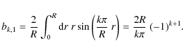
q2(r)=H[r-r1], which yields for the emission coefficients (26)
,
the spatial injection function is
q2(r)=H[r-r1], which yields for the emission coefficients (26)
We then find for the synchrotronintensity
![$\displaystyle (r_1,\epsilon,t)\simeq\frac{c\sigma_{\rm T}q_0B^2\gamma_0R}{6\pi^...
... s}\right]}{\sqrt{E_0\epsilon}}~
\frac{H\left[E_0-\epsilon\right]}{t-t_{\rm s}}$](/articles/aa/full_html/2010/03/aa12966-09/img160.png)
![$\displaystyle \times~ H\left[\frac{2R}{c}+t_{\rm s}-t\right]~
\exp\left(-\frac{g(x)c}{R}(t-t_{\rm s})\right)~\sum^{k_{\max}}_{k=1}\frac{1}{k^3}$](/articles/aa/full_html/2010/03/aa12966-09/img161.png)
which is shown in Fig. 2 for b=0.05 and two values of r1 for soft (
Similar to the first injection scenario we see a steeper rise for the X-rays photons, but to a lower maximum intensity. However, now the light curves in both energy ranges exhibit two maxima in the case of
| Figure 2:
Temporal flare behaviour of optical photons a) and soft X-rays b) resulting from
a homogeneous electron injection over the outer shell
|
|
| Open with DEXTER | |
6 Conclusions
In the previous sections we have investigated an analytic model describing the intrinsic
synchrotron intensity emitted by a spherical plasmoid volume in the jet of an AGN.
Analytical results for the emergent synchrotronintensity are
possible because we have used the monochromatic approximation for the synchrotronpower. The synchrotronintensity is
given by an infinite sum, reflecting the spatial eigenfunction distribution of the radiating electrons
over the emission knot. The sum of eigenfunctions results from the time-dependent spatial diffusion of
electrons subject to synchrotronenergy losses. The radiative transport of the generated synchrotronphotons is simplified
by using the escape probability concept, which approximates the spatial photon diffusion caused by multiple
Compton scatterings off thermal electrons in the knot. With these assumptions we
demonstrate that (1) the total duration of the synchrotron flare at all photon energies ![]() is 2R/c,
(2) shorter photon energy-dependent synchrotronintensity time variations are possible, which reflect the influence of the
photon retardation and escape as well as the temporal and spatial dependences of the relativistic electron
density distribution, and (3) the starting time of the synchrotron flare at photon energy
is 2R/c,
(2) shorter photon energy-dependent synchrotronintensity time variations are possible, which reflect the influence of the
photon retardation and escape as well as the temporal and spatial dependences of the relativistic electron
density distribution, and (3) the starting time of the synchrotron flare at photon energy ![]() is delayed
with respect to the injection time of electrons t0 by the photon energy dependent time scale
is delayed
with respect to the injection time of electrons t0 by the photon energy dependent time scale
![]() ,
reflecting the necessary cooling time
which relativistic electrons need in order to radiate at photon energies below the initial characteristic
synchrotronphoton energy E0.
,
reflecting the necessary cooling time
which relativistic electrons need in order to radiate at photon energies below the initial characteristic
synchrotronphoton energy E0.
The result (2) indicates that time variability different from a single peak in the synchrotronlight curves is possible even with a single electron injection if photon retardation and electron propagation effects are properly taken into account. We illustrate this by choosing different spatial distributions of the electron accelerators in the source. By using future accurate synchrotronlight curves one thus may infer, either by forward trial-and-error calculations or by inversion methods, the true accelerator locations.
AcknowledgementsWe thank the referee for her/his valuable comments. This work was partially supported by the Deutsche Forschungsgemeinschaft through grants RH 35/6-1 and SCHL 201/20-1.
Appendix A: Reduction of the integral (46)
With the use of
![]() ,
the integral (46) becomes
,
the integral (46) becomes
![\begin{displaymath}J(t,r)=\int^R_0 {\rm d}r' ~ \sin(\lambda_kr') ~
H\left[r'+r-u\right]~H\left[u-\left\vert r-r'\right\vert\right].
\end{displaymath}](/articles/aa/full_html/2010/03/aa12966-09/img167.png)
Because of the Heaviside functions, the integral has to be examined in three different ranges, as seen in Fig. A.1, which yields
![\begin{eqnarray*}J(t,r)&=&H\left[u\right]\biggl\lgroup H\left[r-u\right]~ \int^R...
...ight]~ \int^R_{u+r} {\rm d}r' ~ \sin(\lambda_kr') \biggr\rgroup.
\end{eqnarray*}](/articles/aa/full_html/2010/03/aa12966-09/img168.png)
As the cosine is an even function, the first two integrals could be merged to one in the range of
![\begin{eqnarray*}J(t,r)&=&\frac{H\left[u\right]}{\lambda_k}\biggl\lgroup H\left[...
...(\lambda_kR)-\cos\bigl(\lambda_k(r+u)\bigr)\Bigr) \biggr\rgroup.
\end{eqnarray*}](/articles/aa/full_html/2010/03/aa12966-09/img170.png)
![\begin{figure}
\par\includegraphics[width=6.5cm,clip]{12966fg3.eps}
\end{figure}](/articles/aa/full_html/2010/03/aa12966-09/img171.png)
|
Figure A.1:
The grey area illustrates the range of integration.
The lower limit r'=u-r is given by H[r'+r-u].
|
| Open with DEXTER | |
Appendix B: invariance relations
The transformation formulae regarding photon intensities result
from the Lorentz invariance of the photon phase space density (Begelman et al. 1984)

With the photon energy-momentum relation
For the differential photon density
so that the intensity I=c M relation is
Times and photon energies transform as
References
- Aharonian, F. A., et al. (HESS Collaboration) 2007, ApJ, 664, L7 [Google Scholar]
- Albert, J., Aliu, E., Anderhub, H., et al. (MAGIC Collaboration) 2007, ApJ, 663, 125 [NASA ADS] [CrossRef] [Google Scholar]
- Begelman, M. C., Blandford, R. D., & Rees, M. J. 1984, Rev. Mod. Phys., 56, 2 [Google Scholar]
- Coppi, P. S. 1992, MNRAS, 258, 657 [NASA ADS] [CrossRef] [Google Scholar]
- Crusius, A., & Schlickeiser, R. 1986, A&A, 164, 16 [Google Scholar]
- Crusius, A., & Schlickeiser, R. 1988, A&A, 196, 327 [NASA ADS] [Google Scholar]
- Fabian, A. C., Blandford, R. D., Guilbert, P. W., Phinney, E. S., & Cuellar, L. 1986, MNRAS, 221, 931 [NASA ADS] [CrossRef] [Google Scholar]
- Felten, J. E., & Morrison, P. 1966, ApJ, 146, 686 [NASA ADS] [CrossRef] [Google Scholar]
- Gould, R. J. 1979, A&A, 76, 306 [NASA ADS] [Google Scholar]
- Lightman, A. P., & Zdziarski, A. A. 1987, ApJ, 319, 643 [NASA ADS] [CrossRef] [Google Scholar]
- Piner, B. G., & Edwards, P. G. 2004, ApJ, 600, 115 [NASA ADS] [CrossRef] [Google Scholar]
- Schlickeiser, R. 1996, Space Sci. Rev., 75, 299 [NASA ADS] [CrossRef] [Google Scholar]
- Schlickeiser, R. 2009, MNRAS, 398, 1483 [NASA ADS] [CrossRef] [Google Scholar]
- Schlickeiser, R., & Lerche, I. 2007, A&A, 476, 1 [NASA ADS] [CrossRef] [EDP Sciences] [Google Scholar]
- Schlickeiser, R., & Röken, C. 2008, A&A, 477, 701 (SR) [NASA ADS] [CrossRef] [EDP Sciences] [Google Scholar]
- Schlickeiser, R., Vainio, R., Böttcher, M., et al. 2002, A&A, 393, 69 [NASA ADS] [CrossRef] [EDP Sciences] [Google Scholar]
- Stockem, A., & Schlickeiser, R. 2008, ApJ, 680, 816 [NASA ADS] [CrossRef] [Google Scholar]
- Sunyaev, R. A., & Titarchuk, L. G. 1980, A&A, 86, 121 [NASA ADS] [Google Scholar]
- Sunyaev, R. A., & Titarchuk, L. G. 1985, A&A, 143, 374 [NASA ADS] [Google Scholar]
- Turner, M., et al. 2003, Connecting Quarks with the Cosmos (Washington: The National Academic Press) [Google Scholar]
- Woo, J.-H., Urry, C. M., van der Marel, R. P., Lira, P., & Maza, J., et al. 2005, ApJ, 631, 762 [NASA ADS] [CrossRef] [Google Scholar]
All Figures
|
|
Figure 1: Intrinsic synchrotronlight curves of hard X-rays (solid line), soft X-rays (dashed line) and optical photons (dotted line) resulting from a homogeneous electron injection in the whole plasmoid volume of the size of R15=1 and the magnetic field strength of b=0.1. |
| Open with DEXTER | |
| In the text | |
| |
Figure 2:
Temporal flare behaviour of optical photons a) and soft X-rays b) resulting from
a homogeneous electron injection over the outer shell
|
| Open with DEXTER | |
| In the text | |
|
|
Figure A.1:
The grey area illustrates the range of integration.
The lower limit r'=u-r is given by H[r'+r-u].
|
| Open with DEXTER | |
| In the text | |
Copyright ESO 2010
Current usage metrics show cumulative count of Article Views (full-text article views including HTML views, PDF and ePub downloads, according to the available data) and Abstracts Views on Vision4Press platform.
Data correspond to usage on the plateform after 2015. The current usage metrics is available 48-96 hours after online publication and is updated daily on week days.
Initial download of the metrics may take a while.