| Issue |
A&A
Volume 510, February 2010
|
|
|---|---|---|
| Article Number | A101 | |
| Number of page(s) | 11 | |
| Section | Astrophysical processes | |
| DOI | https://doi.org/10.1051/0004-6361/200913520 | |
| Published online | 18 February 2010 | |
On the shape of the spectrum of cosmic rays accelerated inside superbubbles
G. Ferrand1 - A. Marcowith2
1 - Laboratoire Astrophysique Interactions Multi-échelles (AIM),
CEA/Irfu, CNRS/INSU, Université Paris VII, L'Orme des
Merisiers, Bât. 709, CEA Saclay, 91191 Gif-sur-Yvette
Cedex, France
2 - Laboratoire de Physique Théorique et Astroparticules (LPTA),
CNRS/IN2P3, Université Montpellier II, Place Eugène Bataillon,
34095 Montpellier Cedex, France
Received 21 October 2009 / Accepted 16 November 2009
Abstract
Context. Supernova remnants are believed to be a
major source of energetic particles (cosmic rays)
on the Galactic scale. Since their progenitors, namely the most massive
stars, are commonly found clustered in OB associations,
one has to consider the possibility of collective effects in the
acceleration process.
Aims. We investigate the shape of the spectrum of
high-energy protons produced inside the superbubbles
blown around clusters of massive stars.
Methods. We embed simple semi-analytical models of
particle acceleration and transport inside Monte Carlo simulations of
OB associations timelines. We consider regular acceleration
(Fermi 1 process) at the shock front of supernova remnants, as
well as stochastic reacceleration (Fermi 2 process) and escape
(controlled by magnetic turbulence) occurring between the shocks. In
this first attempt, we limit ourselves to linear acceleration by strong
shocks and neglect proton energy losses.
Results. We observe that particle spectra, although
highly variable, have a distinctive shape because of the competition
between acceleration and escape: they are harder at the lowest energies
(index s<4) and softer at the highest
energies (s>4). The momentum at which this
spectral break occurs depends on the various bubble parameters, but all
their effects can be summarized by a single dimensionless parameter,
which we evaluate for a selection of massive star regions in the Galaxy
and the LMC.
Conclusions. The behaviour of a superbubble in terms
of particle acceleration critically depends on the magnetic turbulence:
if B is low then the superbubble is simply the host of a
collection of individual supernovae shocks, but if B is high
enough (and the turbulence index is not too high), then the superbubble
acts as a global accelerator, producing distinctive spectra, that are
potentially very hard over a wide range of energies, which has
important implications on the high-energy emission from these objects.
Key words: acceleration of particles - shock waves - turbulence - cosmic rays - ISM: supernova remnants
1 Introduction
Superbubbles are hot and tenuous large structures that are formed around OB associations by the powerful winds and the explosions of massive stars (Higdon & Lingenfelter 2005). They are the major hosts of supernovae in the Galaxy, and thus major candidates for the production of energetic particles (e.g., Bykov 2001; Montmerle 1979; Butt 2009, and references therein). Supernovae are indeed believed to be the main contributors of Galactic cosmic rays (along with pulsars and micro-quasars), by means of the diffusive shock acceleration process (a 1st-order, regular Fermi process) occurring at the remnant's blast wave as it goes through the interstellar medium (Malkov & Drury 2001; Drury 1983).
Supernovae in superbubbles are correlated in space and time, hence the need to investigate acceleration by multiple shocks (Parizot et al. 2004). Klepach et al. (2000) developed a semi-analytical model of test-particle acceleration by multiple spherical shocks (either wind termination shocks, or supernova shocks plus wind external shocks), based on the limiting assumption of small shocks filling factors. Ferrand et al. (2008) performed direct numerical simulations of repeated acceleration by successive planar shocks in the non-linear regime (that is, taking into account the back-reaction of energetic particles on the shocks). However, to ascertain the particle spectrum produced inside the superbubble as a whole, one must also consider important physics occurring between the shocks. Since the bubble interior is probably magnetized and turbulent, we need to evaluate gains and losses caused by the acceleration by waves (a 2nd-order, stochastic Fermi process) and escape from the bubble.
In this study, we combine the effects of regular acceleration (occurring quite discreetly, at shock fronts) and stochastic acceleration and escape (occurring continuously, between shocks), to determine the typical spectra that we can expect inside superbubbles over the lifetime of an OB cluster. We choose to treat regular acceleration as simply as we can, and concentrate on modeling the relevant scales of stochastic acceleration and escape inside superbubbles. We present our model in Sect. 2, give our general results in Sect. 3, and present specific applications in Sect. 4. Finally we discuss the limitations of our approach in Sect. 5 and provide our conclusions in Sect. 6.
2 Model
Our model is based on Monte Carlo simulations of the activity of a
cluster of massive stars, in which we embed simple semi-analytical
models of (re-)acceleration and escape
(described by means of their Green functions).
To evaluate the average properties of a cluster of ![]() stars,
we perform random samplings of the initial mass function
(Sect. 2.1).
For a given cluster, time is sampled in intervals
stars,
we perform random samplings of the initial mass function
(Sect. 2.1).
For a given cluster, time is sampled in intervals ![]() ,
which is short enough to ensure that at most one supernova occurs
during that period,
but by chance for large clusters, and which is long enough to consider
that
regular acceleration at a shock front has shaped the spectrum of
particles
- acceleration is thought to take place mostly at early stages of
supernova remnant evolution,
and in a superbubble the Sedov phase begins after a few thousands of
years (Parizot et al. 2004).
Here we do not try to investigate the exact extent of the spectrum
of accelerated particles: we set the lowest momentum (injection
momentum)
to be
,
which is short enough to ensure that at most one supernova occurs
during that period,
but by chance for large clusters, and which is long enough to consider
that
regular acceleration at a shock front has shaped the spectrum of
particles
- acceleration is thought to take place mostly at early stages of
supernova remnant evolution,
and in a superbubble the Sedov phase begins after a few thousands of
years (Parizot et al. 2004).
Here we do not try to investigate the exact extent of the spectrum
of accelerated particles: we set the lowest momentum (injection
momentum)
to be ![]() (which is the typical thermal
momentum downstream of a supernova shock) and set the highest momentum
(escape momentum) to be
(which is the typical thermal
momentum downstream of a supernova shock) and set the highest momentum
(escape momentum) to be ![]() (which
corresponds to the ``knee'' break in the spectrum of cosmic rays as
observed on the Earth). We note that the theoretical acceleration time
from
(which
corresponds to the ``knee'' break in the spectrum of cosmic rays as
observed on the Earth). We note that the theoretical acceleration time
from ![]() to
to ![]() (in the linear regime,
without escape) is roughly 8000 yr (assuming Bohm diffusion
with
(in the linear regime,
without escape) is roughly 8000 yr (assuming Bohm diffusion
with
![]() G), which is
again consistent with our choice of
G), which is
again consistent with our choice of ![]() .
This corresponds to 8 decades in p, at a
resolution of a
few tens of bins per decade (according to Sect. 2.2.2).
.
This corresponds to 8 decades in p, at a
resolution of a
few tens of bins per decade (according to Sect. 2.2.2).
The procedure is then as follows: for each time bin in the
life of the cluster,
either (1) a supernova occurs, and the distribution of
particles evolves according to the diffusive shock acceleration
process, as explained in Sect. 2.2;
or (2) no supernova occurs, and the distribution evolves
taking into account acceleration and escape controlled by magnetic
turbulence, as explained in Sect. 2.3.
This process is repeated for many random clusters of the same size,
until some average trend emerges regarding the shape of spectra (note
that average spectra are not monitored for each bin ![]() but in
larger steps of 1 Myr).
but in
larger steps of 1 Myr).
In the following, we describe our modeling of massive stars, supernovae shocks, and magnetic turbulence.
2.1 OB clusters: random samplings of supernovae
We are interested in massive stars that die by core-collapse, producing
type Ib, Ic or II supernovae, that
is of mass greater than ![]() ,
and up to say
,
and up to say ![]() .
These are stars of spectral type O (>
.
These are stars of spectral type O (>
![]() )
and include stars of spectral type B (
)
and include stars of spectral type B (
![]() ).
Most massive stars spend all their life within the cluster in which
they were born, forming OB associations. To describe the
evolution of such a cluster, one needs to know the distribution of star
masses and lifetimes.
).
Most massive stars spend all their life within the cluster in which
they were born, forming OB associations. To describe the
evolution of such a cluster, one needs to know the distribution of star
masses and lifetimes.
The initial mass function (IMF) ![]() is defined so that the number of stars in the mass interval
m to
is defined so that the number of stars in the mass interval
m to ![]() is
is ![]() ,
so that the number of stars of masses between
,
so that the number of stars of masses between ![]() and
and ![]() is
is
![]() Observations
show that
Observations
show that ![]() can be expressed as a power law (Salpeter
1955)
can be expressed as a power law (Salpeter
1955)
with an index of
Stars lifetimes can be computed from stellar evolution models,
and here we use data from Limongi
& Chieffi (2006), which is plotted in Fig. 2.
The more massive they are, the faster stars burn their material. A star
at the threshold ![]() has a lifetime of
has a lifetime of ![]() ,
which is also the total lifetime of the cluster;
a star of
,
which is also the total lifetime of the cluster;
a star of ![]() lives only
lives only ![]() .
Regarding supernovae, the active lifetime of the cluster is thus
.
Regarding supernovae, the active lifetime of the cluster is thus
![\begin{figure}
\par\includegraphics[width=8.5cm,clip]{13520_1.eps}
\end{figure}](/articles/aa/full_html/2010/02/aa13520-09/img43.png)
|
Figure 1:
Distribution of massive stars masses: the initial mass function.
For each cluster |
| Open with DEXTER | |
![\begin{figure}
\par\includegraphics[width=8.5cm,clip]{13520_2.eps}
\end{figure}](/articles/aa/full_html/2010/02/aa13520-09/img44.png)
|
Figure 2: Distribution of massive stars lifetimes (data from Limongi & Chieffi 2006). |
| Open with DEXTER | |
2.2 Supernovae shocks: regular acceleration
2.2.1 Green function
To keep things as simple as possible, we limit ourselves here to the
test-particle approach
(non-linear calculations will be presented elsewhere).
In the linear regime, we know the Green function G1
that links the distributions![]() of particles
downstream and upstream of a single shock according to
of particles
downstream and upstream of a single shock according to
it reads
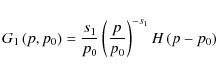
where H is the Heaviside function, and

where r is the compression ratio of the shock.
2.2.2 Adiabatic decompression
Around an OB association, particles produced by a supernova shock might be reaccelerated by the shocks of subsequent supernova before they escape the superbubble. The effect of repeated acceleration is basically to harden the spectra (Achterberg 1990; Melrose & Pope 1993).
When dealing with multiple shocks, it is mandatory
to account for adiabatic decompression between the shocks: the momenta
of energetic particles bound to the fluid will decrease by a factor R=r1/3
when the fluid density decreases by a factor r. To
resolve decompression properly, the numerical momentum resolution ![]() has to be significantly smaller than the induced momentum shift (Ferrand et al. 2008).
has to be significantly smaller than the induced momentum shift (Ferrand et al. 2008).
2.3 Magnetic turbulence: stochastic acceleration and escape
Particles accelerated by supernova shocks, although energetic,
might remain for a while inside the superbubble because of magnetic
turbulence
that scatters them (they perform a random walk until they escape).
Because of this turbulence, particles will also experience stochastic
reacceleration during their stay in the bubble. We present here a
deliberately simple model of transport, to obtain the relevant
functional dependences and order of magnitudes of the diffusion
coefficients.
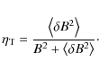
The turbulent magnetic field ![]() is represented by its power spectrum W(k),
defined so that
is represented by its power spectrum W(k),
defined so that ![]() ,
where
,
where ![]() ,
,
![]() is the
turbulence scale,
and
is the
turbulence scale,
and ![]() (respectively
(respectively ![]() )
corresponds to waves interacting with the particles of highest
(respectively lowest) energy. This spectrum is usually taken to be a
power law of index q
)
corresponds to waves interacting with the particles of highest
(respectively lowest) energy. This spectrum is usually taken to be a
power law of index q

normalised by the turbulence level
2.3.1 Diffusion scales
If the turbulence follows Eq. (6), then the space
diffusion coefficient is given by
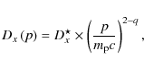
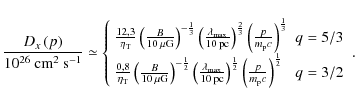
where we assume that the turbulence spectrum extends sufficiently for this description to remain correct at the lowest particle energies. Using results from Casse et al. (2002) obtained for isotropic turbulence, one can assume that
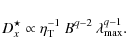
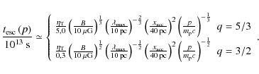
For standard turbulence indices, we obtain
Particles diffuse over a typical length scale of
where
For standard turbulence indices, we obtain
Interaction with waves also leads to a diffusion in momentum. Using results from quasi-linear theory, we can express the diffusion coefficient as
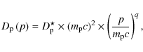
where
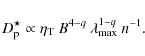
and n is the number density (which determines the Alfvén velocity together with B). For standard turbulence indices, we obtain
|
(16) |
2.3.2 Green function
Becker et al. (2006)
presented the first analytical expression of the Green function G2
for both stochastic acceleration and escape
that is valid for any turbulence index ![]() .
It is defined so that, for impulsive injection of distribution
.
It is defined so that, for impulsive injection of distribution ![]() ,
the distribution after time t is
,
the distribution after time t is
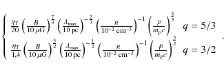
Neglecting losses, it can be expressed as
where
G2 represents the
distribution of particles remaining inside the bubble.
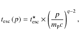
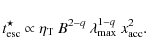
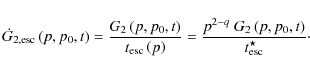
One can also evaluate the rate of particles escaping the bubble by
dividing G2 by the escape
time given by Eq. (11):
3 Results
3.1 Distribution of supernovae shocks
Before presenting the spectra of particles, we briefly discuss the temporal distribution of shocks during the life of the cluster, because this controls the possibility of repeated acceleration.
3.1.1 Rate of supernovae
As an illustration of our Monte Carlo procedure, if we count the number
of supernovae in each time bin ![]() ,
we can estimate the mean supernovae rate. The result is shown in
Fig. 3.
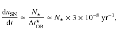
In agreement with the ``instantaneous burst'' model of Cerviño et al. (2000),
we observe that the distributions of masses and lifetimes
combine in such a way that, but for a peak at the beginning, the rate
of supernovae is fairly constant
during the cluster's life, and can be expressed to a first
approximation by
,
we can estimate the mean supernovae rate. The result is shown in
Fig. 3.
In agreement with the ``instantaneous burst'' model of Cerviño et al. (2000),
we observe that the distributions of masses and lifetimes
combine in such a way that, but for a peak at the beginning, the rate
of supernovae is fairly constant
during the cluster's life, and can be expressed to a first
approximation by
where we recall that
![\begin{figure}
\par\includegraphics[width=8.2cm,clip]{13520_3.eps}
\end{figure}](/articles/aa/full_html/2010/02/aa13520-09/img89.png)
|
Figure 3:
Mean supernovae rate as a function of time.
For each cluster, |
| Open with DEXTER | |
3.1.2 Typical time between shocks
Knowledge of the time distribution of supernovae is important to
acceleration
in superbubbles, because, depending on the typical interval between
shocks, accelerated particles may or may not remain within the bubble
between two supernovae explosions, and thus experience repeated
acceleration![]() . We thus monitor the time
interval
. We thus monitor the time
interval ![]() between two successive supernovae. The result is
shown in Fig. 4.
We note that (1) the most probable time interval between
two shocks is simply the average time between two supernovae
between two successive supernovae. The result is
shown in Fig. 4.
We note that (1) the most probable time interval between
two shocks is simply the average time between two supernovae ![]() and
(2) when time intervals are normalised by this quantity,
all distributions have the same shape independently of the number
of stars (apart from very low numbers of stars).
and
(2) when time intervals are normalised by this quantity,
all distributions have the same shape independently of the number
of stars (apart from very low numbers of stars).
To investigate the probability of acceleration by many
successive shocks, we now compute the maximum time ![]() that a particle has to wait within a sequence of n
successive shocks. Only particles whose escape
time is longer than this value may experience acceleration by n
shocks. As previously, all distributions have the same shape once time
intervals are normalised by
that a particle has to wait within a sequence of n
successive shocks. Only particles whose escape
time is longer than this value may experience acceleration by n
shocks. As previously, all distributions have the same shape once time
intervals are normalised by ![]() ,
and are very peaked,
but now the most probable value of
,
and are very peaked,
but now the most probable value of ![]() is a few times longer than the average value (the more successive
shocks we consider, the higher the probability
of obtaining an unusually long time interval between any two of them).
This is summarised in Fig. 5,
which shows
the most probable value of
is a few times longer than the average value (the more successive
shocks we consider, the higher the probability
of obtaining an unusually long time interval between any two of them).
This is summarised in Fig. 5,
which shows
the most probable value of ![]() as a function of the number of successive shocks. We note that
as a function of the number of successive shocks. We note that ![]() may reach 10 times
may reach 10 times ![]() ,
and that it is an imprecise indicator when
,
and that it is an imprecise indicator when ![]() and n are low.
and n are low.
![\begin{figure}
\par\includegraphics[width=8.2cm,clip]{13520_4.eps}
\end{figure}](/articles/aa/full_html/2010/02/aa13520-09/img94.png)
|
Figure 4:
Distribution of the interval between two successive shocks (normalised
to the average interval between two supernovae).
For each cluster, the interval between two successive
supernova is monitored, within the numerical resolution |
| Open with DEXTER | |
![\begin{figure}
\par\includegraphics[width=8.2cm,clip]{13520_5.eps}
\end{figure}](/articles/aa/full_html/2010/02/aa13520-09/img95.png)
|
Figure 5:
Maximum time interval between two successive shocks in a sequence of n
successive shocks (normalised to the average interval between two
supernovae).
Solid curves correspond to the most frequent value of |
| Open with DEXTER | |
![\begin{figure}
\par\includegraphics[width=8.5cm,clip]{13520_6a.eps}\hspace*{4mm}...
...eps}\hspace*{4mm}
\includegraphics[width=8.5cm,clip]{13520_6f.eps}
\end{figure}](/articles/aa/full_html/2010/02/aa13520-09/img101.png)
|
Figure 6:
Sample results of average spectra of cosmic rays inside the
superbubble.
The particles spectrum f and its logarithmic slope |
| Open with DEXTER | |
3.2 Average cosmic-ray spectra
3.2.1 General trends
![\begin{figure}
\par\includegraphics[width=8.5cm,clip]{13520_7a.eps}\hspace*{4mm}
\includegraphics[width=8.5cm,clip]{13520_7b.eps}
\end{figure}](/articles/aa/full_html/2010/02/aa13520-09/img102.png)
|
Figure 7:
Sample results of average spectra of cosmic rays escaping the
superbubble.
The particles spectrum f per unit time and its
logarithmic slope |
| Open with DEXTER | |
Hard spectra at low energies are produced by the combined effects of acceleration by supernova shocks (Fermi 1) and reacceleration by turbulence (Fermi 2). Soft spectra at high energies are mostly shaped by escape, which preferentially removes highly energetic particles. The transition energy is controlled by a balance between reacceleration and escape timescales, and thus depends on the superbubble parameters.
3.2.2 Parametric study
![\begin{figure}
\par\mbox{\includegraphics[width=5.8cm,clip]{13520_8a.eps}\hspace*{4mm}
\includegraphics[width=5.8cm,clip]{13520_8b.eps} }\end{figure}](/articles/aa/full_html/2010/02/aa13520-09/img105.png)
|
Figure 8:
Hard-soft transition momentum as a function of |
| Open with DEXTER | |
![\begin{figure}
\par\mbox{\includegraphics[width=5.8cm,clip]{13520_9a.eps}\hspace*{4mm}
\includegraphics[width=5.8cm,clip]{13520_9b.eps} }\end{figure}](/articles/aa/full_html/2010/02/aa13520-09/img108.png)
|
Figure 9:
Lowest slope as a function of |
| Open with DEXTER | |
For each cluster, we must define eight parameters ![]() ,
r, q,
,
r, q, ![]() ,
B,
,
B, ![]() ,
n, and
,
n, and ![]() ,
which are more or less constrained. We sample the size of the cluster
roughly logarithmically between 10 stars and
500 stars, i.e.
,
which are more or less constrained. We sample the size of the cluster
roughly logarithmically between 10 stars and
500 stars, i.e. ![]() ,
30, 70, 200, 500. We consider only strong supernova shocks of r=4.
We compare the classical turbulence indices q=5/3(Kolmogorov
cascade, K41) and q=3/2 (Kraichnan cascade, IK65).
We consider two different scenarios for the magnetic field: if a
turbulent dynamo
is operating then
,
30, 70, 200, 500. We consider only strong supernova shocks of r=4.
We compare the classical turbulence indices q=5/3(Kolmogorov
cascade, K41) and q=3/2 (Kraichnan cascade, IK65).
We consider two different scenarios for the magnetic field: if a
turbulent dynamo
is operating then ![]() and
and ![]() ,
so that
,
so that ![]() (Bykov 2001); if not, then
because of the bubble expansion
(Bykov 2001); if not, then
because of the bubble expansion ![]() and
and ![]() (if
(if ![]() ,
then
,
then ![]() ). The
external scale of the turbulence
). The
external scale of the turbulence ![]() is at least of the order of the distance
is at least of the order of the distance ![]() between two stars in the cluster, which, for
a typical OB association radius of 35 pc
(e.g., Garmany 1994),
and assuming uniform distribution (a quite crude approximation), is
between two stars in the cluster, which, for
a typical OB association radius of 35 pc
(e.g., Garmany 1994),
and assuming uniform distribution (a quite crude approximation), is

which is 26, 12 and 7 pc for 10, 100 and 500 stars respectively. However,
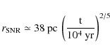
in the Sedov-Taylor phase inside a superbubble (Parizot et al. 2004). Hence, we consider
We thus had to perform many simulations to explore the
parameter space.
However, interestingly, the effects of the 6 parameters
relevant to stochastic acceleration and escape q, ![]() ,
B,
,
B, ![]() ,
n, and
,
n, and ![]() can be
summarized by a single parameter, the adimensional number
can be
summarized by a single parameter, the adimensional number
![]() introduced by Becker
et al. (2006)
introduced by Becker
et al. (2006)

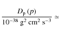
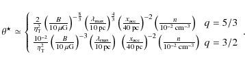
which, according to Eqs. (15) and (12) varies as
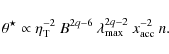
For standard turbulence indices, we have
For all the possible superbubble parameters considered here,
To characterize the spectra of accelerated particles, we use
two indicators, which are plotted in Figs. 8
and 9.
We checked that the results are independent of the resolution, provided
that there is at least a few bins per decompression shift.
The residual variability seen originates mostly in the simulation
procedure itself, which is based on random samplings.
In Fig. 8,
we show the momentum of
transition from hard to soft regimes, defined as the maximum momentum
up to which the slope may be smaller than a given value (3
or 4 here).
Above this momentum, the slope always remains greater than this value.
Below this momentum, the slope can be as low as 0,
meaning that particles pile-up from injection - but we note that it can
also
happen to be ![]() 4
at a particular time in a particular cluster sample, since
distributions are highly variable. As
4
at a particular time in a particular cluster sample, since
distributions are highly variable. As ![]() increases, the transition momentum falls exponentially
from almost the maximum momentum considered (a fraction of PeV)
to the injection momentum (10 MeV). For rule-of-thumb
calculations,
one can say that the slope can be <3 up to
increases, the transition momentum falls exponentially
from almost the maximum momentum considered (a fraction of PeV)
to the injection momentum (10 MeV). For rule-of-thumb
calculations,
one can say that the slope can be <3 up to ![]() GeV.
In Fig. 9,
we show the shallowest slope (corresponding
to the hardest spectrum) obtained at a fixed momentum (1 GeV
and
1 TeV here). As
GeV.
In Fig. 9,
we show the shallowest slope (corresponding
to the hardest spectrum) obtained at a fixed momentum (1 GeV
and
1 TeV here). As ![]() increases, the lowest slope rises from 0 (which is possible in the case
of stochastic reacceleration) to 4 (the canonical value for
single regular acceleration in the test particle case).
As expected, the critical
increases, the lowest slope rises from 0 (which is possible in the case
of stochastic reacceleration) to 4 (the canonical value for
single regular acceleration in the test particle case).
As expected, the critical ![]() between hard and soft regimes decreases as we increase the reference
momentum: the break occurs around
between hard and soft regimes decreases as we increase the reference
momentum: the break occurs around ![]() for
for ![]() ,
and around
,
and around ![]() for
for ![]() .
.
This overall behaviour can be explained by noting that ![]() is roughly
the ratio of the reacceleration time to the escape time. Low
is roughly
the ratio of the reacceleration time to the escape time. Low
![]() are obtained when reacceleration is faster than escape, allowing Fermi
processes to produce hard spectra up to high energies, as particles
become reaccelerated by shocks and/or turbulence.
In contrast, high
are obtained when reacceleration is faster than escape, allowing Fermi
processes to produce hard spectra up to high energies, as particles
become reaccelerated by shocks and/or turbulence.
In contrast, high
![]() are obtained when escape is faster than reacceleration, resulting in
quite soft in-situ spectra,
as particles escape immediately after being accelerated by a supernova
shock.
The case
are obtained when escape is faster than reacceleration, resulting in
quite soft in-situ spectra,
as particles escape immediately after being accelerated by a supernova
shock.
The case ![]() corresponds to a balance between gains and losses,
in the particular case of which the spectral break occurs around
10 GeV for s>4, and around
1 GeV for s>3.
corresponds to a balance between gains and losses,
in the particular case of which the spectral break occurs around
10 GeV for s>4, and around
1 GeV for s>3.
Table 1: Physical parameters for well observed massive-star forming regions in the Galaxy and in the LMC.
4 Application
4.1 A selection of massive star regions
We gathered the physical parameters of some well observed massive star
clusters and their associated superbubbles. The reliability and the
completeness of the data were our main selection criteria. The
parameters useful for our study are: the cluster composition (number of
massive stars), age, distance, size, and the superbubble size and
density. We note that we are biased towards young objects, since older
ones are more difficult to isolate because of their large extensions
and sequential formations. Information about density is sometimes
unavailable. The density can span several orders of magnitude, usually
between 10-2 and
![]() in the central cluster (Torres
et al. 2004), and between 10-3
and
in the central cluster (Torres
et al. 2004), and between 10-3
and ![]() in the superbubble (Parizot
et al. 2004). If X-ray observations are available,
it can be indirectly estimated from the thermal X-ray spectrum, given
the plasma temperature and the column density along the line of sight.
In the case of a complete lack of data, we accept a mean density of
between
in the superbubble (Parizot
et al. 2004). If X-ray observations are available,
it can be indirectly estimated from the thermal X-ray spectrum, given
the plasma temperature and the column density along the line of sight.
In the case of a complete lack of data, we accept a mean density of
between ![]() and
and ![]() .
Unfortunately, the magnetic field parameters can not be directly
measured, so that we consider different limiting scenarios:
.
Unfortunately, the magnetic field parameters can not be directly
measured, so that we consider different limiting scenarios: ![]() and
and ![]() if the turbulence is low, and
if the turbulence is low, and ![]() and
and ![]() if the turbulence is high. In each case, we compare our results for
turbulence indices q=5/3 and q=3/2.
The maximal scale of the turbulence
if the turbulence is high. In each case, we compare our results for
turbulence indices q=5/3 and q=3/2.
The maximal scale of the turbulence ![]() may be taken to be as small as the size of the stellar cluster
(especially in the case where few supernovae have already occurred), or
as large as the superbubble itself.
may be taken to be as small as the size of the stellar cluster
(especially in the case where few supernovae have already occurred), or
as large as the superbubble itself.
These quantities are used to estimate the key parameter ![]() in each of the selected objects using Eq. (25). All the
parameters and results are summarised in Table 1. Before discussing
the implications of these values, we provide details of the selected
regions in the following two sections, regarding clusters found in our
Galaxy and in the Large Magellanic Cloud (LMC), respectively.
in each of the selected objects using Eq. (25). All the
parameters and results are summarised in Table 1. Before discussing
the implications of these values, we provide details of the selected
regions in the following two sections, regarding clusters found in our
Galaxy and in the Large Magellanic Cloud (LMC), respectively.
4.1.1 Galaxy
We selected 6 objects in the Galaxy.
- Cygnus region: in this region we identify two distinct objects, the clusters Cygnus OB1 and OB3, which have blown a common superbubble, and the cluster Cygnus OB2. We note that the latter was detected at TeV energies by Hegra (Aharonian et al. 2005) as an extended source (TeV J2032+4130), and by Milagro (Abdo et al. 2007), as extended diffuse emission and at least one source (MGRO J2019+37). A supershell was also detected around the Cygnus X-ray superbubble, which may have been produced by a sequence of starbursts, Cygnus OB2 being the very last.
- Orion OB1: this association consists of several subgroups (Brown et al. 1999), the age of 12 Myr selected here corresponds to the oldest one (OB1a).
- Carina nebula: this region is one of the most massive star-forming regions in our Galaxy. It contains two massive stellar clusters, Trumpler 14 and Trumpler 16 (Smith et al. 2000), of cumulative size of approximately 10 pc.
- Westerlund 1: this cluster is very compact although it harbours hundreds of massive stars. The size of the superbubble is uncertain, and we assume here the value of 40 pc reported by Kothes & Dougherty (2007) for the HI shell surrounding the cluster. We note that Westerlund 1 was detected by HESS (Ohm et al. 2009).
- Westerlund 2: the distance to this cluster remains
a matter of debate (see the discussion in Aharonian
et al. 2007), and we adopt here the estimate of Rauw et al. (2007),
using it to re-evaluate the size obtained by Conti
& Crowther (2004). We assume that the giant HII
region RCW49 of size 100 pc is the structure blown by
Westerlund 2. Tsujimoto
et al. (2007) provided a spectral fit of the diffuse
X-ray emission from RCW49, from which we deduce a density

 .
We note that Westerlund 2 was detected by HESS (Aharonian et al. 2007).
.
We note that Westerlund 2 was detected by HESS (Aharonian et al. 2007).
4.1.2 Large Magellanic Cloud
We selected 3 objects in the LMC. All density estimates here have been derived from observations of diffuse X-ray emission. At the distance of the LMC, these observations usually cover the entire structure, so that the density deduced is an average over the OB association and the ionised region around it.
- DEML 192: this region harbours two massive star clusters, LH 51 and 54 (Lucke & Hodge 1970). We deduced the spatial extensions of both clusters from Oey & Smedley (1998), but these are probably overestimates, because the edges of the clusters are not clearly defined.
- 30 Doradus: this region is quite complex as can be
seen from Chandra observations (Townsley
et al. 2006). In particular, the superbubble
extension is difficult to estimate precisely. We decided to assume the
value given for the 30 Doradus nebula by Walborn (1991). The extension
of the star cluster may be larger than the core which harbours several
thousands of stars (Massey
& Hunter 1998). The core size is
 10 pc
(Massey & Hunter 1998),
it is even estimated to be
10 pc
(Massey & Hunter 1998),
it is even estimated to be  pc by Walborn (1991). The number of
massive stars in R136 depends on the cluster total mass, estimated to
be between
pc by Walborn (1991). The number of
massive stars in R136 depends on the cluster total mass, estimated to
be between  and
and  .
Using a Salpeter IMF, one finds that
.
Using a Salpeter IMF, one finds that 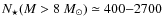 .
We note that the stellar formation in 30 Doradus was
sequential and started more than 10 Myr ago (Massey & Hunter 1998).
.
We note that the stellar formation in 30 Doradus was
sequential and started more than 10 Myr ago (Massey & Hunter 1998).
- N11: this giant HII region harbours several star clusters LH9, LH10, LH13, and LH14, probably produced as a sequence of starbursts (Walborn et al. 1999). Here we mostly consider the star cluster LH9 at the center of N11 and the shell encompassing it (shell 1 in Mac Low et al. 1998). LH10 is a younger star cluster with an estimated age of 1 Myr (Walborn et al. 1999) in which no supernova has yet occurred. The other clusters are less powerful.
4.2 Discussion
In Table 1, we can see that in all cases except for q=3/2,
![]() ,
the critical momentum
,
the critical momentum ![]()
![]() GeV is in the
non-relativistic regime. Even if at lower energies the particle
distribution is hard, since pressure is always dominated by
relativistic particles, one should not expect a strong back-reaction of
accelerated particles over the fluid inside the superbubble, compared
to the case where collective acceleration effects are not taken into
account. However, if the magnetic field pressure is close to
equipartition with the thermal pressure as suggested by Parizot et al. (2004),
and provided that the turbulence index q is
sufficiently low, then the impact of particles on their environment has
to be investigated. More generally, if q is low
enough and/or B is high enough, then the
superbubble can no longer be regarded as a sum of isolated supernovae,
but acts as a global accelerator, producing hard spectra over a wide
range of momenta.
GeV is in the
non-relativistic regime. Even if at lower energies the particle
distribution is hard, since pressure is always dominated by
relativistic particles, one should not expect a strong back-reaction of
accelerated particles over the fluid inside the superbubble, compared
to the case where collective acceleration effects are not taken into
account. However, if the magnetic field pressure is close to
equipartition with the thermal pressure as suggested by Parizot et al. (2004),
and provided that the turbulence index q is
sufficiently low, then the impact of particles on their environment has
to be investigated. More generally, if q is low
enough and/or B is high enough, then the
superbubble can no longer be regarded as a sum of isolated supernovae,
but acts as a global accelerator, producing hard spectra over a wide
range of momenta.
One can wonder how solid these results are, given all the
uncertainties in the data. In particular, the parameter ![]() is very sensitive to the accelerator size
is very sensitive to the accelerator size ![]() .
However
.
However ![]() cannot be much lower than a few tens of parsecs (the typical size of
the OB association) and cannot be much larger than
100 pc (the typical size of the superbubble). The maximal
scale of the turbulence,
cannot be much lower than a few tens of parsecs (the typical size of
the OB association) and cannot be much larger than
100 pc (the typical size of the superbubble). The maximal
scale of the turbulence, ![]() ,
is even more difficult to estimate, but it also ranges between those
extrema. Determining precisely these spatial scales is complicated by
the difficulty of estimating the supershell associated with a given
cluster, all the more so since multiple bursts episodes have occurred
(as is likely the case in 30 Doradus). In addition,
,
is even more difficult to estimate, but it also ranges between those
extrema. Determining precisely these spatial scales is complicated by
the difficulty of estimating the supershell associated with a given
cluster, all the more so since multiple bursts episodes have occurred
(as is likely the case in 30 Doradus). In addition, ![]() is
directly proportional to the density, which is not always measured with
good accuracy, but can usually be rather well constrained to within one
order of magnitude. The upper and lower values of
is
directly proportional to the density, which is not always measured with
good accuracy, but can usually be rather well constrained to within one
order of magnitude. The upper and lower values of ![]() given in Table 1
reflect the uncertainties in these three key parameters. In the end, we
believe that the results presented in Table 1 provide a good
indication of whether or not collective effects will dominate inside
the superbubble. Across the range of possible values of size and
density, the main uncertainty in the critical parameter
given in Table 1
reflect the uncertainties in these three key parameters. In the end, we
believe that the results presented in Table 1 provide a good
indication of whether or not collective effects will dominate inside
the superbubble. Across the range of possible values of size and
density, the main uncertainty in the critical parameter ![]() is clearly due to our poor knowledge of the magnetic field (how strong
the field is, how turbulent it is). It can be seen from Table 1 that for a given
prescription of the magnetic turbulence, the values obtained for both
Galactic and LMC clusters are not very different from one another.
is clearly due to our poor knowledge of the magnetic field (how strong
the field is, how turbulent it is). It can be seen from Table 1 that for a given
prescription of the magnetic turbulence, the values obtained for both
Galactic and LMC clusters are not very different from one another.
5 Limitations and possible extensions
5.1 Regarding shock acceleration physics
The potentially greatest limitation of our model is its use of a linear model for regular acceleration: we have not considered the back-reaction of accelerated particles on their accelerator, whereas cosmic rays may easily modify the supernova remnant shock and therefore the way in which they themselves are accelerated (Malkov & Drury 2001). Since non-linear acceleration is a difficult problem, only a few models are available, such as the time-asymptotic semi-analytical models of Berezhko & Ellison (1999) or Blasi & Vietri (2005), and the time-dependent numerical simulations of Kang & Jones (2007) or Ferrand et al. (2008). We will include one of these non-linear approaches in our Monte Carlo framework in extending our current work. We can already note that non-linear effects tend to produce concave spectra, softer at low energies and harder at high energies than the canonical power-law spectrum, and may thus compete with reacceleration and escape effects that we have shown to have opposite effects. Moreover, non-linearity also occurs regarding the turbulent magnetic field (mandatory for Fermi process to scatter off particles), which remarkably can be produced by energetic particles themselves by various instabilities. This difficult and still quite poorly understood process has been studied by means of MHD simulations (Jones & Kang 2006), semi-analytical models (Amato & Blasi 2006), and Monte Carlo simulations (Vladimirov et al. 2006).
Another limitation is that only strong primary supernova
shocks have been
considered (of compression ratio r=4), but since
superbubbles are very
clumpy and turbulent media, many weak secondary shocks are also
expected
(of r<4). The compression ratio r
depends on the Mach number
![]() according to
according to

where
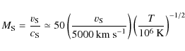
and
Finally, one may question our particular choice of stellar
evolution models,
but we believe that possible variations in the exact lifetime of
massive stars
would bring only higher order corrections to the general picture that
we have obtained.
We also note that we have implicitly considered that stars are born at
the same time,
and then evolve independently, while in reality star formation may
occur through successive bursts within a same molecular cloud, which
could be sequentially
triggered by the first explosions of supernovae. Another possible
amendment to our model is that stars of mass greater than
40 solar masses may end their life without collapsing, and
thus without launching a shock. We have repeated our 720 simulations at
low resolution considering the occurrence of supernovae only for ![]() ,
and checked that our two indicators remain globally unchanged. This
seems consistent with the shape of the IMF (there are very few stars of
very high mass)
and the shape of star lifetimes (stars of very high mass have roughly
the same lifetime).
,
and checked that our two indicators remain globally unchanged. This
seems consistent with the shape of the IMF (there are very few stars of
very high mass)
and the shape of star lifetimes (stars of very high mass have roughly
the same lifetime).
5.2 Regarding inter-shock physics
We use an approximate model of stochastic acceleration,
because of the use of relativistic formulae and the neglect of energy
losses, to be able to use results from Becker
et al. (2006). However, we note that, in terms of
stochastic acceleration, the relativistic regime
is reached when ![]() ,
where v is the particle velocity and
,
where v is the particle velocity and ![]() the Alfvén velocity
the Alfvén velocity
and in a superbubble this condition is met for
Finally, we note that most parameters are time-dependent, and
might become considerably different at late stages.
For completeness, we have performed our simulations until the explosion
of the longest lived stars, but over tens of millions of years the
overall morphology and properties of the superbubble might change
substantially as it interacts with its environment.
As long as the typical evolution timescale of relevant parameters is
longer than our time-step
![]() ,
their variation can be taken into account
simply by varying the value of
,
their variation can be taken into account
simply by varying the value of ![]() accordingly. Otherwise, direct time-dependent numerical simulations
similar to those of Ferrand
et al. (2008)
will be necessary.
accordingly. Otherwise, direct time-dependent numerical simulations
similar to those of Ferrand
et al. (2008)
will be necessary.
6 Conclusions
Our main conclusions are as follows:
- 1.
- Cosmic-ray spectra inside superbubbles are highly variable: at a given time they depend on the particular history of a given cluster.
- 2.
- Nevertheless, spectra follow a distinctive overall trend,
produced by
a competition between (re-)acceleration by regular and stochastic
Fermi processes and escape: they are harder at lower energies (s<4)
and
softer at higher energies (s>4), shapes that
are in agreement with the results of Bykov
(2001) based on different assumptions
![[*]](/icons/foot_motif.png) .
.
- 3.
- The momentum at which this spectral break occurs critically
depends on the bubble parameters:
it increases when the magnetic field value and acceleration region size
increase, and decreases when the density and the turbulence external
scale increase,
all these effects being summarized by the single dimensionless
parameter
 defined by Eq. (23).
- 4.
- For reasonable values of superbubble parameters, very hard spectra (s<3) can be obtained over a wide range of energies, provided that superbubbles are highly magnetized and turbulent (which is a debated issue).
The authors would like to thank Isabelle Grenier and Thierry Montmerle for sharing their thoughts on the issues investigated here.
References
- Abdo, A. A., Allen, B., Berley, D., et al. 2007, ApJ, 658, L33 [Google Scholar]
- Achterberg, A. 1990, A&A, 231, 251 [NASA ADS] [Google Scholar]
- Aharonian, F., Akhperjanian, A., Beilicke, M., et al. 2005, A&A, 431, 197 [Google Scholar]
- Aharonian, F., Akhperjanian, A. G., Bazer-Bachi, A. R., et al. 2007, A&A, 467, 1075 [Google Scholar]
- Aharonian, F. A., & Atoyan, A. M. 1996, A&A, 309, 917 [NASA ADS] [Google Scholar]
- Amato, E., & Blasi, P. 2006, MNRAS, 371, 1251 [NASA ADS] [CrossRef] [Google Scholar]
- Becker, P. A., Le, T., & Dermer, C. D. 2006, ApJ, 647, 539 [Google Scholar]
- Berezhko, E. G., & Ellison, D. C. 1999, ApJ, 526, 385 [NASA ADS] [CrossRef] [Google Scholar]
- Blasi, P., & Vietri, M. 2005, ApJ, 626, 877 [NASA ADS] [CrossRef] [Google Scholar]
- Brandner, W., Clark, J. S., Stolte, A., et al. 2008, A&A, 478, 137 [NASA ADS] [CrossRef] [EDP Sciences] [Google Scholar]
- Brown, A. G. A., Blaauw, A., Hoogerwerf, R., de Bruijne, J. H. J., & de Zeeuw, P. T. 1999, in NATO ASIC Proc. 540: The Origin of Stars and Planetary Systems, ed. C. J. L. N. D. Kylafis, 411 [Google Scholar]
- Brown, A. G. A., de Geus, E. J., & de Zeeuw, P. T. 1994, A&A, 289, 101 [NASA ADS] [Google Scholar]
- Brown, A. G. A., Hartmann, D., & Burton, W. B. 1995, A&A, 300, 903 [NASA ADS] [Google Scholar]
- Burrows, D. N., Singh, K. P., Nousek, J. A., Garmire, G. P., & Good, J. 1993, ApJ, 406, 97 [NASA ADS] [CrossRef] [Google Scholar]
- Butt, Y. 2009, Nature, 460, 701 [NASA ADS] [CrossRef] [PubMed] [Google Scholar]
- Bykov, A. M. 2001, Space Sci. Rev., 99, 317 [Google Scholar]
- Cash, W., Charles, P., Bowyer, S., et al. 1980, ApJ, 238, L71 [NASA ADS] [CrossRef] [Google Scholar]
- Casse, F., Lemoine, M., & Pelletier, G. 2002, Phys. Rev. D, 65, 023002 1 [Google Scholar]
- Cerviño, M., Knödlseder, J., Schaerer, D., von Ballmoos, P., & Meynet, G. 2000, A&A, 363, 970 [NASA ADS] [Google Scholar]
- Conti, P. S., & Crowther, P. A. 2004, MNRAS, 355, 899 [NASA ADS] [CrossRef] [Google Scholar]
- Cooper, R. L., Guerrero, M. A., Chu, Y.-H., Chen, C.-H. R., & Dunne, B. C. 2004, ApJ, 605, 751 [NASA ADS] [CrossRef] [Google Scholar]
- Davidson, K., & Humphreys, R. M. 1997, ARA&A, 35, 1 [NASA ADS] [CrossRef] [Google Scholar]
- Drury, L. O. 1983, Repor. Progr. Phys., 46, 973 [Google Scholar]
- Dunne, B. C., Points, S. D., & Chu, Y.-H. 2001, ApJS, 136, 119 [NASA ADS] [CrossRef] [Google Scholar]
- Ferrand, G., Downes, T., & Marcowith, A. 2008, MNRAS, 383, 41 [NASA ADS] [Google Scholar]
- Garmany, C. D. 1994, PASP, 106, 25 [NASA ADS] [CrossRef] [Google Scholar]
- Hanson, M. M. 2003, ApJ, 597, 957 [NASA ADS] [CrossRef] [Google Scholar]
- Higdon, J. C., & Lingenfelter, R. E. 2005, ApJ, 628, 738 [NASA ADS] [CrossRef] [MathSciNet] [Google Scholar]
- Jones, T. W., & Kang, H. 2006, Cosmic Particle Acceleration, 26th meeting of the IAU, Joint Discussion 1, 16, 17 August, 2006, Prague, Czech Republic, JD01, #41, 1 [Google Scholar]
- Kang, H., & Jones, T. W. 2007, Astroparticle Phys., 28, 232 [Google Scholar]
- Klepach, E. G., Ptuskin, V. S., & Zirakashvili, V. N. 2000, Astroparticle Phys., 13, 161 [Google Scholar]
- Knauth, D. C., Federman, S. R., Lambert, D. L., & Crane, P. 2000, Nature, 405, 656 [NASA ADS] [CrossRef] [PubMed] [Google Scholar]
- Knödlseder, J. 2000, A&A, 360, 539 [NASA ADS] [Google Scholar]
- Knödlseder, J., Cerviño, M., Le Duigou, J.-M., et al. 2002, A&A, 390, 945 [NASA ADS] [CrossRef] [EDP Sciences] [Google Scholar]
- Kothes, R., & Dougherty, S. M. 2007, A&A, 468, 993 [NASA ADS] [CrossRef] [EDP Sciences] [Google Scholar]
- Kroupa, P. 2002, Science, 295, 82 [NASA ADS] [CrossRef] [PubMed] [Google Scholar]
- Limongi, M., & Chieffi, A. 2006, ApJ, 647, 483 [NASA ADS] [CrossRef] [Google Scholar]
- Lozinskaya, T. A., Pravdikova, V. V., Sitnik, T. G., Esipov, V. F., & Mel'Nikov, V. V. 1998, Astron. Rep., 42, 453 [NASA ADS] [Google Scholar]
- Lucke, P. B., & Hodge, P. W. 1970, AJ, 75, 171 [NASA ADS] [CrossRef] [Google Scholar]
- Mac Low, M.-M., Chang, T. H., Chu, Y.-H., et al. 1998, ApJ, 493, 260 [NASA ADS] [CrossRef] [Google Scholar]
- Maddox, L. A., Williams, R. M., Dunne, B. C., & Chu, Y.-H. 2009, ApJ, 699, 911 [NASA ADS] [CrossRef] [Google Scholar]
- Malkov, M. A., & Drury, L. O. 2001, Rep. Progr. Phys., 64, 429 [NASA ADS] [CrossRef] [Google Scholar]
- Massey, P., & Hunter, D. A. 1998, ApJ, 493, 180 [NASA ADS] [CrossRef] [Google Scholar]
- Massey, P., Johnson, K. E., & Degioia-Eastwood, K. 1995, ApJ, 454, 151 [NASA ADS] [CrossRef] [Google Scholar]
- Melrose, D. B. & Pope, M. H. 1993, Proc. Astr. Soc. Aust., 10, 222 [Google Scholar]
- Montmerle, T. 1979, ApJ, 231, 95 [NASA ADS] [CrossRef] [Google Scholar]
- Nazé, Y., Antokhin, I. I., Rauw, G., et al. 2004, A&A, 418, 841 [NASA ADS] [CrossRef] [EDP Sciences] [Google Scholar]
- Nichols-Bohlin, J., & Fesen, R. A. 1993, AJ, 105, 672 [NASA ADS] [CrossRef] [Google Scholar]
- Oey, M. S., & Smedley, S. A. 1998, AJ, 116, 1263 [NASA ADS] [CrossRef] [Google Scholar]
- Ohm, S., Horns, D., Reimer, O., et al. 2009 [arXiv:0906.2637] [Google Scholar]
- Parizot, E., Marcowith, A., van der Swaluw, E., Bykov, A. M., & Tatischeff, V. 2004, A&A, 424, 747 [NASA ADS] [CrossRef] [EDP Sciences] [Google Scholar]
- Rauw, G., Manfroid, J., Gosset, E., et al. 2007, A&A, 463, 981 [NASA ADS] [CrossRef] [EDP Sciences] [Google Scholar]
- Salpeter, E. E. 1955, ApJ, 121, 161 [Google Scholar]
- Selman, F., Melnick, J., Bosch, G., & Terlevich, R. 1999, A&A, 347, 532 [NASA ADS] [Google Scholar]
- Smith, N., Egan, M. P., Carey, S., et al. 2000, ApJ, 532, L145 [NASA ADS] [CrossRef] [PubMed] [Google Scholar]
- Torres, D. F., Domingo-Santamaría, E., & Romero, G. E. 2004, ApJ, 601, L75 [NASA ADS] [CrossRef] [Google Scholar]
- Townsley, L. K., Broos, P. S., Feigelson, E. D., et al. 2006, AJ, 131, 2140 [NASA ADS] [CrossRef] [Google Scholar]
- Tsujimoto, M., Feigelson, E. D., Townsley, L. K., et al. 2007, ApJ, 665, 719 [NASA ADS] [CrossRef] [Google Scholar]
- Vladimirov, A., Ellison, D. C., & Bykov, A. 2006, ApJ, 652, 1246 [NASA ADS] [CrossRef] [Google Scholar]
- Walborn, N. R. 1991, in The Magellanic Clouds, ed. R. Haynes, & D. Milne, IAU Symp., 148, 145 [Google Scholar]
- Walborn, N. R., & Parker, J. W. 1992, ApJ, 399, L87 [NASA ADS] [CrossRef] [Google Scholar]
- Walborn, N. R., Drissen, L., Parker, J. W., et al. 1999, AJ, 118, 1684 [NASA ADS] [CrossRef] [Google Scholar]
- Wang, Q., & Helfand, D. J. 1991, ApJ, 370, 541 [NASA ADS] [CrossRef] [Google Scholar]
Footnotes
- ... distributions
- The distribution function f(p)
is defined so that the particles number density is
 ,
where p is the momentum.
,
where p is the momentum.
- ... acceleration
- Note that this will also strongly depend on the initial energy of the particles: the higher the energy they have gained from one shock, the sooner they will escape the bubble, and hence the smaller chance they have to be reaccelerated by a subsequent shock.
- ... assumptions
- Bykov (2001) considers acceleration of particles by large-scale motions of the magnetized plasma inside the superbubble, which depends on the ratio Du/Dx where Dx is the space diffusion coefficient, controlled by magnetic fluctuations at small scales, and Du=UL describes the effect of large scale turbulence, where U is the average turbulent speed and L is the average size between turbulence sources.
All Tables
Table 1: Physical parameters for well observed massive-star forming regions in the Galaxy and in the LMC.
All Figures
|
|
Figure 1:
Distribution of massive stars masses: the initial mass function.
For each cluster |
| Open with DEXTER | |
| In the text | |
|
|
Figure 2: Distribution of massive stars lifetimes (data from Limongi & Chieffi 2006). |
| Open with DEXTER | |
| In the text | |
|
|
Figure 3:
Mean supernovae rate as a function of time.
For each cluster, |
| Open with DEXTER | |
| In the text | |
|
|
Figure 4:
Distribution of the interval between two successive shocks (normalised
to the average interval between two supernovae).
For each cluster, the interval between two successive
supernova is monitored, within the numerical resolution |
| Open with DEXTER | |
| In the text | |
|
|
Figure 5:
Maximum time interval between two successive shocks in a sequence of n
successive shocks (normalised to the average interval between two
supernovae).
Solid curves correspond to the most frequent value of |
| Open with DEXTER | |
| In the text | |
|
|
Figure 6:
Sample results of average spectra of cosmic rays inside the
superbubble.
The particles spectrum f and its logarithmic slope |
| Open with DEXTER | |
| In the text | |
|
|
Figure 7:
Sample results of average spectra of cosmic rays escaping the
superbubble.
The particles spectrum f per unit time and its
logarithmic slope |
| Open with DEXTER | |
| In the text | |
|
|
Figure 8:
Hard-soft transition momentum as a function of |
| Open with DEXTER | |
| In the text | |
|
|
Figure 9:
Lowest slope as a function of |
| Open with DEXTER | |
| In the text | |
Copyright ESO 2010
Current usage metrics show cumulative count of Article Views (full-text article views including HTML views, PDF and ePub downloads, according to the available data) and Abstracts Views on Vision4Press platform.
Data correspond to usage on the plateform after 2015. The current usage metrics is available 48-96 hours after online publication and is updated daily on week days.
Initial download of the metrics may take a while.